Process Selection - From Design to Manufacture Episode 2 Part 6 pptx

//SYS21///INTEGRAS/B&H/PRS/FINALS_07-05-03/0750654376-CH003.3D – 264 – [249–300/52] 8.5.2003 8:57PM
Fig. 3.14 Chart used for the determination of the section coefficient (
C
s
) for forming processes.
264 Costing designs
//SYS21///INTEGRAS/B&H/PRS/FINALS_07-05-03/0750654376-CH003.3D – 265 – [249–300/52] 8.5.2003 8:57PM
Fig. 3.15 Chart used for the determination of the section coefficient (
C
s
) for plastic molding, continuous extrusion and
machining processes.
Component costing 265
//SYS21///INTEGRAS/B&H/PRS/FINALS_07-05-03/0750654376-CH003.3D – 266 – [249–300/52] 8.5.2003 8:57PM
Fig. 3.16 Chart used for the determination of the tolerance coefficient (
C
t
) for casting processes.
266 Costing designs
//SYS21///INTEGRAS/B&H/PRS/FINALS_07-05-03/0750654376-CH003.3D – 267 – [249–300/52] 8.5.2003 8:57PM
Fig. 3.17 Chart used for the determination of the tolerance coefficient (
C
t
) for forming processes.
Component costing 267
//SYS21///INTEGRAS/B&H/PRS/FINALS_07-05-03/0750654376-CH003.3D – 268 – [249–300/52] 8.5.2003 8:57PM
Fig. 3.18 Chart used for the determination of the tolerance coefficient (
C
t
) for plastic molding, continuous extrusion and
machining processes.

268 Costing designs
//SYS21///INTEGRAS/B&H/PRS/FINALS_07-05-03/0750654376-CH003.3D – 269 – [249–300/52] 8.5.2003 8:57PM
Fig. 3.19 Chart used for the determination of the surface finish coefficient (
C
f
) for casting processes.
Component costing 269
//SYS21///INTEGRAS/B&H/PRS/FINALS_07-05-03/0750654376-CH003.3D – 270 – [249–300/52] 8.5.2003 8:58PM
Fig. 3.20 Chart used for the determination of the surface finish coefficient (
C
f
) for forming processes.
270 Costing designs
//SYS21///INTEGRAS/B&H/PRS/FINALS_07-05-03/0750654376-CH003.3D – 271 – [249–300/52] 8.5.2003 8:58PM
Fig. 3.21 Chart used for the determination of the surface finish coefficient (
C
f
) for plastic molding, continuous extrusion
and machining processes.
Component costing 271
//SYS21///INTEGRAS/B&H/PRS/FINALS_07-05-03/0750654376-CH003.3D – 272 – [249–300/52] 8.5.2003 8:58PM
orthogonal axes or planes (either 1, 2 or 3þ), on which the critical tolerances lie, and which
cannot be achieved from a single direction using the manufacturing process. Repeat the above
process exactly for C
f
using the graphs in Figures 3.19–3.21.
C
ft
¼ C
t

or C
f
, whichever gives the highest value.
Note that for Chemical Milling (CM2.5 and CM5), C
ft
¼ 1, as the penalty is taken account
of in the formulation of the basic processing cost, P
c
.
3.2.4 Material cost (M
c
)
The material cost, M
c
, was defined in Equation (3.1) as the volume of raw material required to
process the component multiplied by the cost of the material per unit volume in the required
form, C
mt
:
M
c
¼ VC
mt
½3:6
Sample average values for C
mt
for commonly used material classes can be found in
Figure 3.22. Company specific data should be used wherever possible. In many situations the
material cost can form a large proportion of the total component cost, therefore a consistent
approach should be taken in the volume calculation if valid comparisons are to be produced.

Note that the volume, V, in Equation (3.6) must be worked out in cubic millimeters (mm
3
).
Reference (1.39) has relative cost data for a number of material classes that can be used where
specific data is not available.
Component manufacture may involve surface coating and/or heat treatments, and have
some effect on manufa cturing cost. Development of models for this aspect of component
manufacturing cost can be found in reference (3.8).
The volume may be calculated in one of two ways:
1 Using the total volume – If the total volume of material required to produce the component
is known (i.e. the volume including an y processing waste), then this value is used for ‘V’ and
the waste coefficient, W
c
, is ignored.
Fig. 3.22 Sample material cost values per unit volume (
C
mt
) for commonly used material classes.
272 Costing designs
//SYS21///INTEGRAS/B&H/PRS/FINALS_07-05-03/0750654376-CH003.3D – 273 – [249–300/52] 8.5.2003 8:58PM
2 Using the final (finished) volume – If the amount of waste material is not known, then the
final component volume may be used. In this case, use the waste coefficient, W
c
, which takes
into account the waste material consumed by a particular process. The formulation for ‘V’
for this method is:
V ¼ V
f
W
c

½3:7
where V
f
is the finished volume of the component.
Waste coefficient, W
c
, for the sample processes can be found in Figure 3.23, relative to
shape classifications provided in Figure 3.9b. While in many cases the values quoted can be
used with confidence, estimation of the input volume to the process is the approach preferred
(method 1 above). In many applications , when calculating the volume of a component, it is
not always necessary to go into great detail. Approximate methods are often satisfactory when
comparing designs, and it can be helpful if a design is broken down into simple shape elements
allowing the quick calculation of a volume. Before looking at the industrial applications of the
design costing methodology it should be noted that material and process selection need to be
considered together, they should not be viewed in isolation. The analysis presented here does
not in any way take into account physical properties such as strength, weight, conductivity, etc.
Note that for Chemical Milling (CM2.5 and CM5), W
c
¼ 1 as the penalty is taken account
of in the formulation of the basic processing cost, P
c
.
3.2.5 Model validation
In order to validate the approach, a number of companies were consulted, covering a wide
range of manufacturing technology and products. Understandably, companie s were often
reluctant to discuss cost information, even admitting that they had no systematic process or
structure to the way new jobs were priced, relying almost exclusively on the knowledge and
expertise of one or two senior estimators. However, a number of companies were able to
provide both estimated and actual cost data for a sufficient range of components to perform
some meaningful validation.

Figure 3.24(a) illustrates the results of a validation exercise in a company producing plastic
molded components. The analysis was performed on a numb er of products at random, and
the estimated costs predicted by the evaluation, M
i
, have been plotted against the actual
manufacturing costs provided by the company. Figure 3.24(b) illustrates another plot, this time
Fig. 3.23 Waste coefficient (
W
c
) for the sample processes relative to shape classification category.
Component costing 273
//SYS21///INTEGRAS/B&H/PRS/FINALS_07-05-03/0750654376-CH003.3D – 274 – [249–300/52] 8.5.2003 8:58PM
Fig. 3.24 Costing methodology validation results.
274 Costing designs
//SYS21///INTEGRAS/B&H/PRS/FINALS_07-05-03/0750654376-CH003.3D – 275 – [249–300/52] 8.5.2003 8:58PM
from a company producing pressed sheet metal parts. Figure 3.25 illustrates some of the
components included in the validation studies.
Validation exercises on a range of component types which was carried out by 22
individuals in industry (mechanical, electrical and manufacturing engineers) showed that
the main variability encountered was in the calculation of component volume and in the
assignment of the shape complexity index (3.9). While the determination of component
volume is mechanistic, it is recognized that the determination of the most appropriate
shape complexity classification requires judgmental skills and experience in the application
of the methodology. These problems were largely eliminated when the analys is was carried
out in a team environment, where highly consistent and reliable results were produced. In
addition, training in the application of the methodology yields considerable improvements
in the quality and consistency of the results produced proving capable of predicting the cost
of manufacture of a component to within 16 per cent. Customizing the data to a particular
business would significantly enhance the accuracy of the predicted costs obtained from the
analysis.

3.2.6 Component costing case studies
One of the primary goals of the technique is to enable a product team to anticipate the cost of
manufacture associated with alternative component design solutions, resulting from the
activities of DFA. The technique is currently used to augment the DFA method exploited
commercially by CSC Manufacturing in the form of DFA consulting projects and as part of
the simultaneous engineering tools and techniques software ‘TeamSET’ (3.10). As mentioned
earlier, one of the main objectives of DFA is the reduction of component numbers in a
product to minimize assembly cost. This tends to generate product design solutions that
contain fewer but sometime s more complex components embodying a number of functions.
Such an approach is often criticized as being sub-optimal; therefore it is important to know
the consequences of such moves on component manufacturing costs. Note that a blank
component costing table is provided in Appendix C.
An illustration of how the design costing analysis can be used in DFA is given in Figures
3.26 and 3.27. Figure 3.26(a) shows the original design of a trim screw assembly and Figure
3.26(b), the replacement design. The DFA analyses can also be seen in Figure 3.26(a) and (b)
respectively. Notice that these figures include data on manufacturing cost and provide the
assembly sequence diagram for each design using the standard ‘TeamSET’ notation. A break-
down of the cost analysis for the two components in the new design of the trim screw is given
in Figure 3.27. Each component has been assigned a manufacturing index which is represen-
tative of the cost in pence. Figure 3.26(c) provides a summary of the resulting measures of
performance for each design. Agai n manufacturing cost values have been included. It can be
seen from this that it is possible to fully assess the production cost consequences of each design
in terms of both component manufacturer and assembly. Note that the total component
manufacturing costs associated with the new design resulting from DFA are less than in the
original: this turns out to be the case in many of the DFA studies examined to date by the
authors.
A simple illustration of a case where the situation is not quite so clear cut is given in Figure
3.28. The DFA approach drives consideration of the assembly design proposal shown in
design ‘B’. An investigation of the two designs using the cost analysis suggests that from a
component manufacturing point of view design ‘A’ represents a cost saving. In this example,

Component costing 275
//SYS21///INTEGRAS/B&H/PRS/FINALS_07-05-03/0750654376-CH003.3D – 276 – [249–300/52] 8.5.2003 8:58PM
Fig. 3.25 Example components used in the validation exercises.
276 Costing designs
//SYS21///INTEGRAS/B&H/PRS/FINALS_07-05-03/0750654376-CH003.3D – 277 – [249–300/52] 8.5.2003 8:58PM
the same manufacturing process (automatic machining) is used for both pin designs, and the
difference in cost results from the different initial material volume requirements. (The values
of P
c
¼ 3 and R
c
¼ 2.75 are the same in each case.) Supplier cost data is used in the case of the
standard clip fasteners. Hence, selection on the basis of cost demands a trade-off between
assembly and manufacturing cost. Both design solutions are commonly seen in products from
various business sectors and product groups.
Comparison of alternative processing routes is illustrated in Figure 3.29. The cold forming
and automatic machining processing routes for the plug body design and production quantity
requirements show significant manufacturing cost variations. The figure presents the detail of
the cost analysis, giving the values obtaine d from P
c
and the individual elements involved in
the calculation of R
c
, together in the table with details of the design. The benefits of the high
material utilization associated with cold forming mean a large cost saving at the annual
production quantity of one million components. (The input volume for the machined compo-
nent is almost five times that required for cold forming.) However, as the annual production
requirement reduces, the processing cost moves more in favor of machining, and at 30 000 per
annum the sample data predicts little difference in cost between the two methods of production
(see lower part of Figure 3.29).

Fig. 3.26 Before and after analysis of a headlight trim screw design.
Component costing 277
//SYS21///INTEGRAS/B&H/PRS/FINALS_07-05-03/0750654376-CH003.3D – 278 – [249–300/52] 8.5.2003 8:58PM
Fig. 3.27 Cost analysis for the manufac ture of the components in the new headlight trim screw design.
278 Costing designs
//SYS21///INTEGRAS/B&H/PRS/FINALS_07-05-03/0750654376-CH003.3D – 279 – [249–300/52] 8.5.2003 8:58PM
Fig. 3.28 Estimated costs for alternative designs of pivot pin components.
Component costing 279
//SYS21///INTEGRAS/B&H/PRS/FINALS_07-05-03/0750654376-CH003.3D – 280 – [249–300/52] 8.5.2003 8:58PM
Fig. 3.29 Comparison of automatic machining and cold forming process es for the manufacture of a plug body.
280 Costing designs
//SYS21///INTEGRAS/B&H/PRS/FINALS_07-05-03/0750654376-CH003.3D – 281 – [249–300/52] 8.5.2003 8:58PM
Fig. 3.30 Comparison of pressure die casting and injection molding processes for the manufacture of a critical surface finish.
Component costing 281
//SYS21///INTEGRAS/B&H/PRS/FINALS_07-05-03/0750654376-CH003.3D – 282 – [249–300/52] 8.5.2003 8:58PM
A case where a material and process change eliminates the need for secondary processing is
shown in Figure 3.30. An aluminum pressure die casting is initially considered for the sleeve
shown, but secondary processing may be needed to ensure conformance to surface finish
requirements as the achievement of 0.4 mm Ra is on the boundary of technical feasibility. An
optional design uses injection molded Polysulfone (PSU). The sample data does not differ-
entiate between plastic injection molding and pressure die casting in terms of basic processing
cost. The savings indicated by the cost analysis result from lower material costs, and surface
finish capability of the injection molding process reflected in C
ft
reduced from 1.5 to 1.05.
Adopting injection molding here removes additional machining and minimizes the complexity
of the manufacturing layout.
The technique can be helpful in producing cost estimates, where design solutions involve a
significant amount of sub-contract work. The estimates produced provide support to the make
versus buy analysis and the technique can be useful in calibrating supplier quotations. Varia-

tions of more than 30 per cent in quotations from sub-contractors against identical specifica-
tions are common across the range of manufacturing processes. This has been noted by a
number of researchers (3.11). In this way benefits can be gained whether the methodology is
applied as a stand-alone tool during product design/redesign or, more globally, as part of a
company’s integrated application of simultaneous engineering tools and techniques. The
applications of the methodology may be summarized as:
.
Determination of component cost in support of DFA
.
Competitor analysis
.
Assistance with make versus buy decisions
.
Cost estimating in concept design with low levels of component detail
.
Support for simultaneous engineering and team-work
.
Training in design for manufacture
3.2.7 Bespoke costing development
Given the wide ranges of process es and their variants, and the problems of producing cost
estimates from generic data that businesses can believe in, it is necessary to explore how we
might go about getting companies to enter their own process knowledge into the component
costing methodology presented previously. In this way, an organization can take ownership of
the process costing knowledge and its maintenance. The development of this process of
‘calibration’ will enable a business to tune the data in the system to known component costs
and take into account problems of varying material and processing cost in different parts of
the world. However, the problem of enabling the user to add new processes to the method-
ology is rather complex. The main difficulties are associated with the need to collect and
represent process knowledge for the calculation of basic processing cost, P
c

and the design
dependent relative cost coefficient, R
c
. The adding of new material costs, M
c
and any
necessary waste coefficients, W
c
is not considered to be a significant problem. The objective
of these notes is to outline a process for the addition of costing information for new processes
to the data-base to facilitate the costing of designs in early stages of the design process.
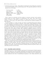
Basic processing cost (P
c
)
In order to determine the basic processing cost, P
c
of a simple or ideal design, it is necessary to
understand the production factors on which it depends. These are equipment costs including
installation, operating costs (labor, supervision and overheads), processing times, tooling
282 Costing designs
//SYS21///INTEGRAS/B&H/PRS/FINALS_07-05-03/0750654376-CH003.3D – 283 – [249–300/52] 8.5.2003 8:58PM
costs and component demand. The above variables are taken account of in the calculation of,
P
c
, using the following equation:
P
c
¼ AT þ B=N ½3:8
where A ¼ total average cost of setting up and operating a specific process, including plant,
labor, supervision and overheads, per second in the chosen country, T ¼ average time in

seconds for the processing of an ideal design for the process , B ¼ average annual cost of
tooling for processing an ideal component, including maintenance and N ¼ total production
quantity per annum.
The above values of A, B and T are based on processing a simple or ideal design well suited
to the process in terms of both material and geometry. They are experience-based quantities
and should be based where possible on established standards and expertise in companies
specializing in the process under consideration.
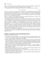
Addition of P
c
data for a new manufacturing process
The steps proposed are as follows:
1 Select a manufacturing process that is currently covered in Part III of the book, and that is
nearest to the new process to be added. For example, consider the adding of reaction
injection moldin g to the system. A similar process would be injection molding.
2 Examine the data used for the quantity ‘A’ for the surrogate process and determine if this
can be used as it stands. If not, decide by how much should it be changed. In the first
instance, this should be checked with sources including published material (manufacturing
books, manuals), manufacturing experts and specialist sup pliers. The average operating
cost of an injection molding facility in the UK is taken as ‘X’. Obtain a view on a
comparative value for reaction injection molding.
3 Repeat process in (2) above for the determination of the value for ‘T ’. The average
operating time for a simple design of component in injection molding is ‘Y’. Obtain a view
on a comparative figure for reaction injection molding.
4 Repeat process in (2) above for the value of ‘B’. The average total tooling cost for injection
molding a simple design in the UK is ‘Z’. Obtain a view on a comparative figure for reaction
injection moldin g.
5 The values obtained above are used to calculate ‘P
c
’ for a range of values for ‘N ’. Produce a
plot for reaction injection molding and compare and discuss.

6 Add the pilot data to the system and represent as such. Add reaction injection molding data
and make as pilot data only.
7 Check the data against known costs for components well suited to the process and calibrate
accordingly. Calibrate the new process to known reaction injection molding case studies.
8 Add data to main database, coded as a new process. The user should be informed that
reaction injection molding cost estimates are based on new data.
9 Once the data is proven, code as a standard process. The user should be informed as such.
Relative cost coefficient (R
c
)
The relative cost coefficie nt is used to determine how much more expensive it will be to
produce a component with more demanding characteristics than the ‘ideal’ design. In order to
determine this quantity, it is necessary to consider the effects of design-dependent criteria.
Component costing 283