Process Selection - From Design to Manufacture Episode 2 Part 5 docx

//SYS21///INTEGRAS/B&H/PRS/FINALS_07-05-03/0750654376-CH002-1.3D – 244 – [35–248/214] 9.5.2003 2:05PM
sensor design is supplied to a leading (tier 1) manufacturer whose generic throttle pedal design
places it well to meet the requirements of many major Original Equipment Manufacturers
(OEM). Given the safety-critical nature of accelerator pedal sensor it is essential to electro-
nically test each completed assembly to make sure it works correctly. The product comprised
eight components and was to be assembled on a 9 s cycle-time.
Process and assembly machine design
The process is essentially automatic, but requires two operators to load critical components.
Each operation is checked to make sure that it took place correctly (any incorrect assemblies
are flagged on the pallet and pass through without further work) . Laser trimming calibrates
the resistance of the unit, and an electronic test also ensures that each completed assem bly
works properly. A modular approach was adopted for the design of the machine. The
operator first loads a housing and rotor onto a flagged pallet. The first automatic station
then loads the substrate, ensures that it is laid flat, and heat stakes it into position. The system
checks only that the substrate is present, not that it performs correctly. Electronic testing of
the final unit is carried out later in the pro cess. Further operations load the spring, rotor and
cover, which are heat staked into position to complete the assembly.
Three of the assembly operations are particularly technically demanding: wire bonding,
spring contact assembly and laser trimmi ng. A proprietary wire bonding station is used to
weld the thin wire contacts into position to link the substrate with the electrical contacts
molded in the sensor body. The spring contact assembly positions three small twin-spoked
contacts and heat stakes them in position. The contacts must be secured without deformation
and a force gauge is used to measure the pressure exerted by every spoke of the contact on the
substrate track to ensure proper con nections are made. Laser trimming of the substrate track
calibrates the final assembly to ensure it has the correct resistance at a reference position. The
system check s the resistance before and after the trimming process. This is a critical operation
that ensures the correct operation of the sensor.
Selection considerations
The assembly technology adopted for the application could be considered as driven by factors
including:
.

High production volumes and continuous demand
.
Very high levels of process capability
.
Complex assembly processes
.
Integrated testing processes.
The product volume and the safety critical nature of the process, coupled with complex
assembly processes point to the need for a special purpose automatic machine with ope rator
loading of critical components.
2.5.3 Joining processes
In order to illustrate the selection methodology, two sample case studies are presented. The case
studies show just how many different joining processes can be used on essentially the same design
and how this affects part-count, assemblability and functional performance in support of DFA.
244 Selecting candidate processes
//SYS21///INTEGRAS/B&H/PRS/FINALS_07-05-03/0750654376-CH002-1.3D – 245 – [35–248/214] 9.5.2003 4:15PM
Case study 1 – Rear windscreen wiper motor
The first case study shows important DFA measures and highlights where joining methods
have had a detrimental effect on the design. The joining process selection methodology has
been applied and the suggested joining processes compared to those used in the DFA rede-
signs. The architecture of the original design is shown in Figure 2.9. The DFA evaluation
shows six functional parts and 23 non-functional parts, givi ng a DFA design efficiency of
17.8 per cent using the Lucas DFA methodology (1.36). Twelve of the non-functional
components are only present for joining and to support the joining method, two bolts and
two nuts to attach the housing and four rivets (and associated spacers) to join the brush plate
to the retaining plate. The motor as intended is a throwaway module, that is, if a failure
occurred during operation, the motor would be replaced, not repaired. Based on this
information, all joints can be stat ed as permanent.
The redesign based on the DFA analysis suggestions is shown in Figure 2.10. The de sign
proposed has six functional components, and no non-functional components, giving a DFA

design efficiency of 100 per cent. The redesign eliminates all twelve components used for joining.
The rivets and spacers have been removed, as the components they join are not in the redesign.
Integrated snap fit fasteners have replaced the nut and bolt assemblies for fastening the housing.
The first step in selecting a joining process from the matrix is to determine the joint’s
requirements. The joint parameters for the housing are high volume (100 000þ), permanent
joint, thermoset material and thin ( 3 mm) material thickness. Based on these constraints, the
selection matrix shows the only suitable process to be a snap fit fastener. However, the
quantity column must also be evaluated for all quantities. This search identifies tubular rivets,
split rivets, compression rivets, nailing, cyanoacrylate adhesives, epoxy resin adhesives, poly-
urethane adhesives and solvent-borne rubber adhesives as alternatives. In this case study, the
geometry and material are unsuitable for riveting and nailing. A comparison of adhesives and
snap fit fasteners indicates that adhesives require more time for application, including a setting
phase, and additional alignment features would need to be built into the components. There-
fore, it is clear that the snap fit fasteners are the most appropriate joining method.
Although the rivets have been removed along with the compo nents they joined, they formed
part of the assembly that held the bearing in place. Consequently, the joint between the
bearing and housing needs to be considered. The joint parameters for the bearing to housing
Fig. 2.9 Motor original design.
Combining the use of the selection strategies and PRIMAs 245
//SYS21///INTEGRAS/B&H/PRS/FINALS_07-05-03/0750654376-CH002-1.3D – 246 – [35–248/214] 9.5.2003 4:15PM
Fig. 2.10 Motor redesign.
are high volume, permanent joint, thermoset and steel material, and thin and medium thick-
ness materials respectively. For this evaluation, the joining processes must match both
material requirements. The search indicated two adhesive types: cyanoacrylate and epoxy
resin as candidates. A search based on the same parameters for all quantities indicates
toughened adhesives as a third candidate. As all the candidate joining processes are similar,
the final decision would be based on process, detailed design requirements and economic
factors, such as cost and availability as provided in the PRIMAs. The proposed redesign
suggested adhesive bonding for fixing the bearing into the housing.
Case study 2 – Gas meter diaphragm assembly

This case study details a sample set of designs from a case study involving 12 designs from
different manufacturers. Here three designs from different manufactures are considered. The
designs incorporate different joining processes for the same problem. Essentially all the designs
are the same with moderately different geometry as shown in Figure 2.11. In each case there is a
top-plate, base-plate, supports for the flow measurement arm and a rubber/fabric diaphragm.
The diaphragm is sandwiched between the base-plate and top-plate with the flow measurement
arm support on top. The joining process used fixes all components together.
The consequences of the joining process selection are highlighted by the influence on part-
count and DFA design efficiency. The design processes can now be compared with the results
from the joining process selection matrix. The joint parameters and results are shown in
Figure 2.12. It must be noted that in cases where two thicknesses are used, a match must be
found for both. Also, although the quantity is high, the ‘ALL QUANTITIES’ column must be
considered. While a permanent joint is required, as the joining strategy is ‘through hole’, it is
also necessary to consider non-permanent solutions.
The matrix results show both riveting and retaining rings (including clips), along with a
number of additional processes as candidates. This example clearly identifies the importance
of selecting the most appropriate joining process. It shows that considering the impact on part-
count and manufacturing processes helps to optimize the fastening of a joint. For example, both
designs B and C use clips, although design C needs two extra pins to form the joint. A possible
redesign would be to combine ideas from designs B and C, by integrating the top plate with the
flow measurement arm support component (incorporating fastening pins as in design B) molded
from a polymer. This would eliminate the separate support component, remove the need for
separate fastening pins and provide location features as part of a functional part.
246 Selecting candidate processes
//SYS21///INTEGRAS/B&H/PRS/FINALS_07-05-03/0750654376-CH002-1.3D – 247 – [35–248/214] 9.5.2003 4:15PM
Fig. 2.11 Diaphragm assembly designs.
The case studies show that selecting an inappropriate joining process can have a large
detrimental effect on a design. It could be argued that a DFA analysis would highlight poor
fastening methods a nd suggest the need for redesign. This point is demonstrated by the
examples shown above; however, a DFA analysis requires a completed design, and while

highlighting the need for redesign, DFA offers no support for generating redesign solutions. If
a proactive DFA approach is to be realized, it is essential that joining process selection be
performed. Apply ing the joining pr ocess selection methodology and supporting data during
product development allows the geometry of components to be tailored to the selec ted joining
process, eliminating the need for redesign.
Combining the use of the selection strategies and PRIMAs 247
//SYS21///INTEGRAS/B&H/PRS/FINALS_07-05-03/0750654376-CH002-1.3D – 248 – [35–248/214] 9.5.2003 2:05PM
Part-count optimization is one of the main aims of DFA, significantly influencing economic
feasibility and often the technical performance of a design. Joining has been proved to have a
large influence on part-count. In many designs, a significant proportion of the components are
only present to support the joining process. Consequently, it can be concluded that a joinin g
selection methodology is an important aspect of DFA. The case studies presented highlight
the importance of joining process selection and its effect on the assemblability of a design. It
can be seen that selecting an appropriate joining process at early stages of the design process
encourages a right-first-time design philosophy, reducing the need for costly redesign work.
Fig. 2.12 Diaphragm assembly joint parameters and re sults.
248 Selecting candidate processes
//SYS21///INTEGRAS/B&H/PRS/FINALS_07-05-03/0750654376-CH003.3D – 249 – [249–300/52] 8.5.2003 8:56PM
Part III
Costing designs
Procedures to enable the exploration of design and process combinations for manufacturing
and assembly cost.
3.1 Introduction
For financial control and successful marketing it is necessary to have cost targets and
realizations throughout the product introduction process. Product cost is virtually always a
prime element in decision making, in manufacturing industry. The main problem in product
introduction is the provision of reliable cost information in the early stages of the design
process, for the comparison of alternative conceptual designs and assessment of the myriad of
ways in which a product may be structured during concept development.
Cost estimates are needed to determine the viability of projects and to minimize project and

product costs. The inadequate nature of the historical standard costing methods and cost
estimating practices found in most companies has been highlighted by researchers over a
number of years (3.1 –3.5). One signal that emerges from all workers is that it is crucial to reject
uneconomic designs early, for it is not often possible to reduce costs productively once
production has commenced, largely due to the high cost of change at this stage in the product
life cycle. Hence, cost analysis is best utilized at the stage in the design process when rough
designs for a component have been prepared.
The aim of the component costing analysis presented here (3.6)(3.7) is to highlight expensive
and difficult to manufacture designs, thus indicating areas that will benefit from further
attention, before the design has been completed. Benefits of the methodology include:
.
Lower component costs
.
Systematic component costing
.
Identification of feasible manufa cturing processes
.
Rapid comparison of alternative designs and competitor products
.
Reduced engineering change
.
Shorter development time and reduced time-to-market
.
Education and training.
The methodology described is ideally applicable to team-based applications, both manu-
ally and in the form of computer software. The initial work was primaril y designed to
cater for components found in the light engineering, aerospace and automotive business
sectors.
The section on assembly costing is intended to support the process of assembly-orientated
design through the provision of assembly performance metrics. As with conventional DFA

//SYS21///INTEGRAS/B&H/PRS/FINALS_07-05-03/0750654376-CH003.3D – 250 – [249–300/52] 8.5.2003 8:56PM
approaches, the methodology allows the user to match designed features with typical assembly
situations (and associated penalties) on charts for each aspect of the assembly analysis. In this
way ambiguity is reduced, and the user may identify features that are of high penalty and
redesign these where necessary. The assembly cost measure should not strictly be taken as an
absolute value. In practice, assembly costs are difficult to quantify and measure, and correla-
tion requires testing a large number of industrial case studies. Nevertheless, the analysis results
are useful when used in a relative mode of application.
3.2 Component costing
In order to produce a practical and widely applicable tool for designers with the capability to
provide feedback on the technological and economic consequences of component design
decisions, it was considered useful to develop a sample model that is widely applicable to a
number of different manufacturing processes. In addition, the model was designed such that
appropriate manufacturing processes and equipment requirements can be specified early in the
product introduction process. Recognizing the problem, that the relationship between a design
and its manufacturing feasibility and cost, is not easily amenable to precise scientific formula-
tion; the model has come out of knowledge-engineering work in a number of user companies
and those specializing in particular manufacturing techniques.
3.2.1 Development of the model
The model is logically based on material volume and processing considerations. The process
cost is determined using a basic processing cost (the cost of producing an ideal design for that
process) and design-dependent relative cost coefficients (which enable any component design
to be compared with the ideal). Material costs are calculated taking into account the trans-
formation of material to yield the final form.
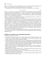
Thus a single process model for manufacturing cost, M
i
, can be formulated as:
M
i
¼ VC

mt
þ R
c
P
c
½3:1
where V is the volume of material required in order to produce the component, C
mt
is the cost
of the material per unit volume in the required form, P
c
is the basic processing cost for an ideal
design of component by a specific process and R
c
is the relative cost coefficient assigned to a
component design (taking account of shape complexity, suitability of material for processing,
section dimensions, tolerances and surface finish).
The initial hypothesis can be expanded to allow for secondary proc essing, and thus the
model can take the general form:
M
i
¼ VC
mt
þðR
c
1
P
c
1
þ R

c
2
P
c
2
þÁÁÁþR
c
n
P
c
n
Þ
M
i
¼ VC
mt
þ
X
n
i ¼ 1
ðR
c
i
P
c
i
Þ½3:2
where n is the number of operations required to achieve the finished component.
In order for such a formulation to be used in practice it is necessary to define relationships
enabling the determination of the quantities P

c
and R
c
for design-process combinations. In
practice, it has been found that Equation (3.1) is the form preferred by industry. This is based
on the need to work in the early stages of the design process with incomplete component data
250 Costing designs
//SYS21///INTEGRAS/B&H/PRS/FINALS_07-05-03/0750654376-CH003.3D – 251 – [249–300/52] 8.5.2003 8:56PM
and without the necessity for detailing the sequence of manufacturing operations. The
approach has been to build the secondary processing requirements into the relative cost
coefficient. More will be said about this in Section 3.2.3.
3.2.2 Basic processing cost (P
c
)
In order to represent the basic processing cost of an ideal design for a particular process, it is
first necessary to identify the factors on which it is dependent. These factors include:
.
Equipment costs including installation
.
Operating costs (labor, number of shifts worked, supervision and overheads, etc.)
.
Processing times
.
Tooling costs
.
Component demand
The above variables are taken account of in the calculation of P
c
using the simple equation:
P

c
¼ T þ =N ½3:3
where a is the cost of setting up and operating a specific process, including plant, labor,
supervision and overheads, per second,  is the process specific total tooling cost for an ideal
design, T is the process time in seconds for processing an ideal design of component by a
specific process and N is the total production quantity per annum.
Values for a and  are based on expertise from companies specializing in producing
components in specific technological areas. Using these process specific values in Equation
(3.3), it is possible to produce comparative cost curves for any process.
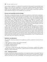
Data for P
c
against annual production quantity, N, is illustrated in Figures 3.1–3.5 for
several main process groups (casting and molding, forming, machining, continuous extrusion
and chemical milling) covering 20 individual manufacturing processes. While the data pre-
sented might be adequate in most cases, the methodology was devised with the idea that users
would develop their own data for the process they would wish to consider. Such an approach
has many benefits to a business, including ownership of the data and a confidence in the
results produced. The values of P
c
represent the minimum likely costs associated with a
particular manufacturing process at a given annual production quantity. In this way, it is
possible to indicate the lowest likely cost for a component associated with a particular
manufacturing process route assuming an ideal design for the process, one-shift working
and a two-year payback on investment.
A process key for the figures is provided below:
AM Automatic Machining
CCEM Cold Continuous Extrusion (Metals)
CDF Closed Die Forging
CEP Continuous Extrusion (Plastics)
CF Cold Forming

CH Cold Heading
CM2.5 Chemical Milling (2.5 mm depth)
CM5 Chemical Milling (5 mm depth)
CMC Ceramic Mold Casting
CNC Computer Numerical Controlled Machining
Component costing 251
//SYS21///INTEGRAS/B&H/PRS/FINALS_07-05-03/0750654376-CH003.3D – 252 – [249–300/52] 8.5.2003 8:56PM
CPM Compression Molding
GDC Gravity Die Casting
HCEM Hot Continuous Extrusion (Metals)
IC Investment Casting
IM Injection Molding
MM Manual Machining
PDC Pressure Die Casting
PM Powder Metallurgy
SM Shell Molding
SC Sand Casting
SMW Sheet Metal Work
VF Vacuum Forming
Having defined P
c
, it is necessary to determine the design-dependent factors. The vari-
ables, shape complexity, tolerances, etc. modify the relationship between the curves. The
relative cost coefficient R
c
in Equation (3.1) is one way in which these variables can be
expressed.
Fig. 3.1 Basic processing cost (
P
c

) against annual production quantity (
N
) for casting and molding processes.
252 Costing designs
//SYS21///INTEGRAS/B&H/PRS/FINALS_07-05-03/0750654376-CH003.3D – 253 – [249–300/52] 8.5.2003 8:56PM
3.2.3 Relative cost coefficient (R
c
)
This coefficient will determine how much more expensive it will be to produce a component
with more demanding features than the ‘ideal design’. The characteristics which we have
assumed to influence the relative cost coefficient, R
c
, are given below:
R
c
¼ fðC
mp
; C
c
; C
s
; C
t
; C
f
Þ
where C
mp
is the relative cost associated with material-process suitability, C
c

is the relative
cost associated with producing components of different geometrical complexity, C
s
is the
relative cost associated with size considerations and achieving component section reductions/
thickness, C
t
is the relative cost associated with obtaining a specified tolerance and C
f
is the
relative cost associated with obtaining a specified surface finish.
Analysis of the influence of the above quantities and discussions with experts led to the idea
that these could be combined as shown below:
R
c
¼ C
a
mp
C
b
c
C
c
s
C
d
t
C
e
f

½3:4
Fig. 3.2 Basic processing cost (
P
c
) against annual production quantity (
N
) for forming processes.
Component costing 253
//SYS21///INTEGRAS/B&H/PRS/FINALS_07-05-03/0750654376-CH003.3D – 254 – [249–300/52] 8.5.2003 8:56PM
where a, b, c, d and e are weighting exponents. However, it was found that the knowledge
could be structured to enable each of the exponents to be assigned the value of unity. There-
fore, the relative cost coefficient can be repres ented by the formula:
R
c
¼ C
mp
C
c
C
s
C
ft
½3:5
where C
ft
is the higher of C
f
and C
t
, but not both.

This was refined on the basis that when a fine surface finish is being produced, fine
tolerances could be attained at the same time, and thus it would be somewhat dubious to
compound both relative cost coefficients.
Knowledge engineering indicated that Equation (3.5) was the most appropriate combi-
nation of coefficients at the present stage of development. The method of comparison and
accumulation of costs was shown to be analogous to those methodologies employed by
experts in the field of cost engineer ing/estimating. For the ideal design, each of these c oeffi-
cients is unity, but as the component design moves away from this state, then one or more of
the coefficients may increase in magnitude, thus changing the manufacturing c ost term, M
i
,in
Equation (3.1).
Figure 3.6 shows how the cost curves for P
c
are modified according to the model proposed,
as a component design shifts away from the ideal for that process. As the design becomes more
difficult to process, because of material types or geometrical features for example, its cost
curve progresses up the cost axis as illustrated, moving from Design A to B in the figure.
Fig. 3.3 Basic processing cost (
P
c
) against annual production quantity (
N
) for machining processes.
254 Costing designs
//SYS21///INTEGRAS/B&H/PRS/FINALS_07-05-03/0750654376-CH003.3D – 255 – [249–300/52] 8.5.2003 8:56PM
Sets of data for the above relative cost coefficients C
mp
, C
c

, C
s
, C
t
and C
f
can be found in
Figures 3.8, 3.9, 3.10, 3.11 and 3.12 respectively.
Material to process suitability (C
mp
)
In Figure 3.7, the C
mp
data indicates the suitability of using various materials with different
processes. Clearly some combinations are inappropriate, and C
mp
values only appear at nodes
currently considered to be technologically and economically feasib le.
Shape complexity (C
c
)
Figures 3.8 and 3.9 present a system to identify the shape classification used, in order to
determine C
c
. The first step is to read the supporting notes and complexity definitions
provided in Fig ure 3.8. There are three basic shape categories: solid of revolution, prismatic
solid and flat or thin wall section components. These three fundamental shape categories can
be sub-divided into five bands of complexity as shown pictorially in Figure 3.9. The classifica-
Fig. 3.4 Basic processing cost (
P

c
) against annual production quantity (
N
) for continuous extrusion processes.
Component costing 255
//SYS21///INTEGRAS/B&H/PRS/FINALS_07-05-03/0750654376-CH003.3D – 256 – [249–300/52] 8.5.2003 8:56PM
tion process must reflect the finished form of the component, and the features listed in the
tables should be used as an aid to the selection of the appropriate value of C
c
from Figures
3.10, 3.11 or 3.12 for classification categories ‘A’, ‘B’ or ‘C’ respectively. Determination of the
shape complexity is important. Failure to classify the geometry properly may affect the final
component cost result, M
i
, quite significantly, and studying the shape complexity definitions is
crucial in this connection.
Section coefficient (C
s
)
Figures 3.13, 3.14 and 3.15 show the relative cost consequences of producing specific section/
wall thicknesses for the sample set of pr ocesses. Data required are the maximum dimension
where the section acts, and the specified section size. Using a process outside its normal size
domain can result in an additional cost. In the situation where a process is being considered
for a component that is longer or smaller than the size range given in the macro (length, area,
volume or weight), the estimate of cost produced is likely to be a lower bound value. Note that
for Chemical Milling (CM2.5 and CM5), C
s
¼ 1, as this penalty is taken account of in the
formulation of the basic processing cost, P
c

.
Fig. 3.5 Basic proces sing cost (
P
c
) against annual production quantity (
N
) for chemical milling.
256 Costing designs
//SYS21///INTEGRAS/B&H/PRS/FINALS_07-05-03/0750654376-CH003.3D – 257 – [249–300/52] 8.5.2003 8:56PM
Tolerance (C
t
) and surface finish (C
f
) coefficients
The sample data on the effects of tolerance (C
t
) and surface finish (C
f
) can be found in Figures
3.16–3.18 and Figures 3.19–3.21 respectively. These indicate the relative cost consequences of
achieving specific tolerance and surface finish levels for the various manufacturing processes.
The process of analysis is:
1 Determine the most important tolerance values.
2 Identify the tolerance band on the C
t
table.
3 Count the number of tolerances in the same band.
4 Identify the number of planes on which the critical values lie.
5 Select the appropriate C
t

index from the table.
Fig. 3.6 Relative manufacturing cost versus quantity curves.
Component costing 257
//SYS21///INTEGRAS/B&H/PRS/FINALS_07-05-03/0750654376-CH003.3D – 258 – [249–300/52] 8.5.2003 8:56PM
Fig. 3.7 Relative cos t data for material processing suitability (
C
mp
).
Fig. 3.8 Notes on shape classification used in the determination of
C
c
.
258 Costing designs
//SYS21///INTEGRAS/B&H/PRS/FINALS_07-05-03/0750654376-CH003.3D – 259 – [249–300/52] 8.5.2003 8:56PM
Fig. 3.9 Shape classification categories used in the determination of
C
c
.
Component costing 259
//SYS21///INTEGRAS/B&H/PRS/FINALS_07-05-03/0750654376-CH003.3D – 260 – [249–300/52] 8.5.2003 8:56PM
Fig. 3.10 Determination of shape complexity coefficient (
C
c
) ^ category ‘A’shape classification.
260 Costing designs
//SYS21///INTEGRAS/B&H/PRS/FINALS_07-05-03/0750654376-CH003.3D – 261 – [249–300/52] 8.5.2003 8:56PM
Fig. 3.11 Determination of shape complexity coefficient (
C
c
) ^ category ‘B’shape classification.

Component costing 261
//SYS21///INTEGRAS/B&H/PRS/FINALS_07-05-03/0750654376-CH003.3D – 262 – [249–300/52] 8.5.2003 8:56PM
Fig. 3.12 Determination of shape complexity coefficient (
C
c
) ^ category ‘C’shape classification.
262 Costing designs
//SYS21///INTEGRAS/B&H/PRS/FINALS_07-05-03/0750654376-CH003.3D – 263 – [249–300/52] 8.5.2003 8:57PM
If the tolerance falls to the left of the thick gray line, a final machining, lapping, honing,
polishing or grindi ng process is necessary to achieve the tolerance. This is already taken into
account in the indices shown. Only the tightest tolerance required should be used, even if
it only occurs on one plane. Included in the graph are separate lines for the number of
Fig. 3.13 Chart used for the determination of the section coefficient (
C
s
) for casting processe s.
Component costing 263