Metal Machining - Theory and Applications Episode 2 Part 3 pot

Simulation of BUE formation 233
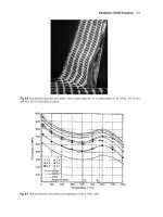
Fig. 8.4 Experimental distorted grid pattern from a quick stop test at a cutting speed of 25 m/min,
f
=0.16 mm,
d
=4 mm,
α
=10º and without coolant
Fig. 8.5 Relation between flow stress and temperature of the 0.18%C steel
Childs Part 2 28:3:2000 3:16 pm Page 233
above 600˚C is so steep that deformation occurs easily. The secondary flow zone grid lines
in Figure 8.1(a), compared with those in Figure 8.3(a), indicate the collapse of the BUE-
range stagnant flow. The almost uniform secondary shear flow stress in Figure 8.1(c) can
be attributed to compensation between work hardening and thermal softening. It indicates
why, despite varying strain, strain rate and temperature along the rake face, split-tool tests
show a plateau friction stress almost independent of distance from the cutting edge
(although this does, of course, depend on the constitutive law chosen for the simulation, as
has been discussed in Chapter 7.4).
In summary, the BUE formation process in steels has successfully been simulated using
the finite element method. Under practical cutting conditions where a BUE appears, the
chip flow property characterized by blue brittleness assists in developing the secondary
shear flow into a stagnant zone. At the boundary between the developed stagnant flow and
the main body of the chip, conditions of high strain concentration, low hydrostatic pres-
sure and material brittleness are favourable for the separation of flow to form the nucleus
of a BUE. The stagnant flow degenerates at higher cutting speeds because thermal soften-
ing prevails over work hardening.
8.2 Simulation of unsteady chip formation
Three examples of unsteady chip formation are described: (1) chip flow, force and resid-
ual stress variations in the low speed (13 mm/min) machining of a b-brass
(60%Cu–40%Zn), in conditions that lead to discontinuous chip formation (Obikawa et al.,
1997); (2) changes in chip formation, and resulting changes in tool fracture probability,

during transient chip flow at the end of a cut, for the low speed machining of a different b-
brass, in conditions which give continuous chip formation (Usui et al., 1990); and (3)
serrated chip formation in machining a Ti-6Al-4V alloy (Obikawa and Usui, 1996). The
treatment of unsteady flow is as outlined in Chapter 7.3.3.
Low strain rate mechanical testing showed both brass materials had the same work-
hardening behaviour, but that which gave discontinuous chips was less ductile than the
other. The low cutting speed of the application means that the effects of strain rate and
temperature on flow stress can be neglected. However, it is found that the distribution of
strain rate in the primary shear zone influences where a crack initiates – and the depen-
dence of shear fracture on this cannot be neglected. The following expressions for flow
stress s
—
dependence on strain e
—
and of fracture criterion on hydrostatic pressure p and
strain rate e
—
˘
(relative to cutting speed, to accommodate the distribution effect) are used for
positive shear of both brasses in the finite element analysis:
p e
—
˘
s
—
(MPa) = 740(e
—
+ 0.01)
0.27
; e

—
≥ a + 0.4 —– – 0.01 — (8.1a)
s
—
V
with a = 1.57 for the less, and 10.0 for the more, ductile material, and V the cutting speed
in mm/s. Friction between the chip and the tool is modelled according to equation (2.24c),
with m and m both equal to 1.
The fracture due to negative shear at the end of a cut occurs under mixed modes: tensile
mode I and shear mode II. The latter is the predominant mode, but the former accelerates
crack propagation. Under the conditions that strain rate due to positive shear is less than
234 Applications of finite element analysis
Childs Part 2 28:3:2000 3:16 pm Page 234
that due to negative shear and that a crack nucleates only in the negative shear region,
another criterion is applied for the negative shear fracture (Obikawa et al., 1990):
p
e
—
≥ 1.1 + 0.3 — (8.1b)
s
—
For the Ti-alloy example, strain rate and temperature effects cannot be ignored. The
material’s flow stress is given in Appendix 4; the shear fracture criterion used is
p(MPa) T(K) e
—
˘
e
—
≥ ——— + 0.09 exp
(

——
)
– MAX
[
0.075log
(
——
)
,0
]
(8.2)
12 600 293 100
where MAX[ , ] means the greater of the two choices. Rake face friction is modelled in the
same way as for the b-brass, with m = 1 but m = 0.6. (The fracture criterion and that for the
b-brass are empirically developed – further developments may be expected in the coming
years, in parallel with flow stress modelling improvements as described in Chapter 7.)
8.2.1 Discontinuous chip formation with a b-brass
Figure 8.6 shows the chip formation predicted at different cut distances L for the b-brass,
with the material properties of equation (8.1a), machined with a carbide tool of rake angle
15˚, at a feed of 0.25 mm. A shear-type discontinuous chip is simulated, with a crack initi-
ating periodically at the tool side of the chip, within the highly deformed workpiece, and
propagating towards the free surface side. Figure 8.7 shows the pattern of changing cutting
forces. Both horizontal and vertical components increase with cut distance, up to the point
where a crack initiates. The crack propagates, accompanied by falling forces. It finally
Simulation of unsteady chip formation 235
Fig. 8.6 Predicted discontinuous chip in
β
-brass machining: cutting speed of 13 mm/min,
f
=0.25 mm,

d
=1 mm,
α
=15º and no coolant
Childs Part 2 28:3:2000 3:16 pm Page 235
penetrates through the chip with a sharp drop in the forces. The force cycle then repeats
itself. These tendencies are in accord with experiments (Obikawa et al., 1997).
Residual stress and strain in the machined layer can also be predicted, as shown in
Figure 8.8. It shows contours of (a) normal stress s
x
acting in the cutting direction and (b)
equivalent plastic strain e
—
, after a cut distance of 5.09 mm and after the cutting forces on
236 Applications of finite element analysis
Fig. 8.7 Predicted horizontal and vertical cutting forces for the same conditions as Figure 8.6
Fig. 8.8 Residual stress and strain in machined layer: (a) direct stress
σ
x
acting in the cutting direction, (b) equivalent
plastic strain; and (c)
σ
x
in continuous chip formation
Childs Part 2 28:3:2000 3:16 pm Page 236
the chip have been relaxed. Periodic variations in s
x
and e
—
occur synchronously with the

cutting force variations (Figure 8.7). For comparison, Figure 8.8(c) shows the continuous
chip and the steady residual stress distribution s
x
obtained by removing the possibility of
fracture from the simulation.
8.2.2 Tool exit transient chip flow
Figure 8.9 shows changes in chip flow as a cutting tool approaches work-exit conditions
(as has been schematically represented in Figure 3.18(b)). Machining with the alumina
Simulation of unsteady chip formation 237
Fig. 8.9 Changes of chip shape and tool edge fracture probability at exit, when machining a
β
-brass with an alumina
ceramic tool at a cutting speed of 13 mm/min,
f
= 0.25 mm,
d
= 3 mm,
α
= 20º, clearance angle
γ
= 5º, exit angle
= 90º, friction coefficient
µ
= 1.0 and no coolant
Childs Part 2 28:3:2000 3:17 pm Page 237
tool is begun only 2.5 mm from its end point: in Figure 8.9(a) (L = 1.09 mm) the chip is
still in its transient initial formation phase; in Figure 8.9(b) (L = 1.79 mm), material flow
into the chip has slowed down as the alternative possibility takes over, of pushing out the
end face of the work, by shear at a negative shear plane angle, to form a burr. Eventually
(Figure 8.9(c)), a crack forms at the clearance surface and propagates along the negative

shear plane towards the end face (Figure 8.9(d)).
The figure also records the changing rake face contact stresses as the end of the cut is
approached. The internal stresses have been determined from these by an elastic finite
element analysis; and used to assess the probability of tool fracture. The contours within
each tool outline are surfaces of constant probability of fracture within a unit volume of
0.01 mm
3
, derived from the principal stress distribution in the tool and the tool material’s
Weibull statistics of failure (Usui et al., 1979, 1982 – see also Chapter 9.2.4). The overall
fractional probability of fracture, G, is given by
n
G = 1 –
P
(1 – G
i
) (8.3a)
i=1
with
1 s* – s
u
m
——
∫
(
———
)
dV (s* ≥ s
u
)
V

0 V
i
s
0
G
i
=
{
(8.3b)
0(s* < s
u
)
where n is the number of finite elements, and G
i
is the probability of fracture within one
element i, V
0
is a unit volume, V
i
is the volume of element i, s* is a scalar stress defined
in Usui’s Weibull statistics model of failure (see Figure 9.8(b)) and s
u
, s
0
and m are
Weibull parameters. In the case of Figure 8.9, G reaches its maximum value of 0.077 at L
= 1.79 mm, just before the crack is formed beneath the cutting edge. Once the crack prop-
agates, compressive tool stresses are created, on the tool’s clearance face, that reduce the
fracture probability. The workpiece fracture relieves the probability of tool fracture; thus,
the friction coefficient m and workpiece brittleness have a strong influence on the tool frac-

ture probability. Reduction of m from 1.0 to 0.6 increases the shear plane angle to delay
negative shear and work crack initiation. This results in an increase in fracture probability,
up to a maximum value of 0.293. On the other hand, if a crack initiates early due to work-
piece brittleness, as in the machining of a cast iron, a low tool fracture probability is
obtained. In cutting experiments, acoustic emission is always detected, when a tool edge
fractures, just before the work negative shear band crack forms (Usui et al., 1990).
In Figure 8.9, the exit angle q, which is the angle between the cutting direction and the
face through which the tool exits the work, is 90˚. Fracture probability is largest for q in
the range 70˚ to 100˚. Smaller exit angles give rise to safe exit conditions (from the point
of view of tool fracture) with little burr formation. Larger angles also give safe exit but
large burr formation. Tool exit conditions are of particular interest in milling and drilling.
In face milling, the exit angle depends on the ratio of radial depth of cut to cutter diame-
ter (d
R
/D, Figure 2.3) and is well-known to affect tool fatigue failures (Pekelharing, 1978).
In drilling through-holes, breakthrough occurs at high exit angles (although the three-
dimensional nature of the breakthrough makes this statement a simplification of what actu-
ally occurs) – and burr formation is a common defect.
238 Applications of finite element analysis
Childs Part 2 28:3:2000 3:17 pm Page 238
8.2.3 Titanium alloy machining
Figure 8.10 shows the pattern of changing chip shape with cut distance L when an a + b
type Ti-6Al-4V alloy is machined with a carbide tool at a cutting speed of 30 m/min, simu-
lated with the material properties described at the start of Section 8.2. A serrated chip
formation is seen. In this case, fractures start at the free surface but never penetrate
completely through the chip.
Figure 8.11 shows temperature distributions within the workpiece and tool at the vari-
ous cut distances corresponding to those in Figure 8.10. Despite a relatively low cutting
speed, the temperature in the chip is high, as has been explained in Chapter 2.3. In that
chapter, only steady state heat generation was considered. An additional effect of non-

steady flow (Figure 8.11(c)) is to bring the maximum temperature rise into the body of the
chip, close to the cutting edge.
Many researchers (for example Recht, 1964; Lemaire and Backofen,1972) have attrib-
uted serrated chip formation in titanium alloy machining to adiabatic shear or thermal soft-
ening in the primary and secondary zones. The results shown in Figures 8.10 and 8.11
contradict this, revealing that the serration arises from the small fracture strain of the alloy,
followed by the propagation of a crack and the localization of deformation. However, if the
fracture criterion is omitted from a simulation, serrated chip formation can still be
observed, but only at higher cutting speeds, for example at 600 m/min (Sandstrom and
Hodowany, 1998). It is clear that fracture and adiabatic heating are different mechanisms
that can both lead to serrated chip formation. In the case of the titanium alloy, serrated
chips occur at cutting speeds too low for adiabatic shear – and then fracture is the cause.
However, at higher speeds, the mechanism and form of serration may change, to become
adiabatic heating controlled.
Simulation of unsteady chip formation 239
Fig. 8.10 Predicted serrated chip shape in titanium alloy machining by a carbide tool, at a cutting speed of 30 m/min,
f
= 0.25 mm,
d
=1 mm,
α
= 20º and no coolant
Childs Part 2 28:3:2000 3:17 pm Page 239
With other alloy systems, for example some ferrous and aluminium alloys, and with other
titanium alloys too, continuous chips may be observed at low cutting speeds, but serrated or
segmented chips are seen at high or very high speeds. In some of these cases, serration is
almost certainly controlled by adiabatic heating and thermal softening, although in the case
of a medium carbon low-alloy steel machining simulation, initial shear fracture has been
observed to aid flow localization and facilitate the onset of adiabatic shear (Marusich and
Ortiz, 1995; Marusich, 1999); and the importance of fracture in concentrating shear is more

strongly argued by some (Vyas and Shaw, 1999). Although the relative importance of frac-
ture and adiabatic shear in individual cases is still a matter for argument, it is certain that an
ideally robust finite element simulation software should have the capacity to deal with ductile
fracture processes even if, in many applications, the fracture capability remains unused.
8.3 Machinability analysis of free cutting steels
The subject of free cutting steels – steels with more sulphur and manganese than normal
(to form manganese sulphide – MnS), and sometimes also with lead additions – was intro-
duced in Chapter 3. Figure 3.16 shows typical force reductions and shear plane angle
increases at low cutting speeds of these steels, relative to a steel without additional MnS
and Pb. These changes have been attributed to embrittling effects of the MnS inclusions in
the primary shear zone (for example Hazra et al., 1974) and a rake face lubricating effect
(for example Yamaguchi and Kato, 1980). The lubrication effect has been considered in
Chapter 2 (Figure 2.23). The deposition of sulphide and other non-metallic inclusions on
240 Applications of finite element analysis
Fig. 8.11 Isotherms near the cutting tip, cutting conditions as Figure 8.10
Childs Part 2 28:3:2000 3:17 pm Page 240
the tool face to reduce wear has also been described (Figure 3.17) and briefly referred to
in Chapter 4 – many researchers have studied this (for example Naylor et al., 1976;
Yamane et al., 1990). Finite element analysis provides a tool for studying the relations
between the cutting conditions (speed, feed, rake angle) and the local stress and tempera-
ture conditions in which the lubricating and wear reducing effects must operate. The next
sections describe a particular comparative investigation into the machining of four steels:
a plain carbon steel, two steels with MnS additions and one steel with MnS and Pb. In this
case, the lubrication effects completely explain observed behaviours, with no evidence of
embrittlement (Maekawa et al., 1991).
8.3.1 Flow and friction properties of resulphurized steels
The compositions of the four steels are listed in Table 8.1. They are identified as P (plain),
X and Y (the steels with MnS added) and L (the steel with MnS and Pb). The steels X and
Y differ in the size of their MnS inclusions: Table 8.1 also gives their inclusion cross-
section areas.

The flow behaviours of the steels in their as-rolled state were found from Hopkinson-
bar compression tests at temperatures T, strain rates e
—
˘
and strains e
—
from 20 to 700˚C, 500
to 2000 s
–1
and 0 to 1, respectively, as described in Chapter 7.4. Figure 8.12 shows the
orientation and size of the specimens: a bar-like test piece of ∅6 mm × 10 mm was cut
from the commercial steel bars that were later machined. Figure 8.13 shows example flow
stress–temperature curves, at a strain rate of 1000 s
–1
and two levels of strain, 0.2 and 1.0.
The symbols indicate measured values while the solid lines are fitted to equation (7.15a).
For the sake of clarity, only the approximated curve for steel P is drawn in the figure. The
flow stress is more or less the same for all four steels, although that for steel X, with larger
MnS inclusions, is slightly lower than that of the others. The values of A, M, N, a and m
(equation (7.15a)) for the steels are listed in Table 8.2.
Machinability analysis of free cutting steels 241
Table 8.1 Chemical composition of workpiece (wt%)
C Mn P S Pb MnS size
(
µ
m
2
)
Steel P 0.100 0.400 0.025 0.019 – –
Steel X 0.070 0.970 0.067 0.339 – 145

Steel Y 0.070 0.910 0.087 0.321 – 124
Steel L 0.080 1.300 0.070 0.323 0.025 –
Fig. 8.12 Specimen preparation for high speed compression testing
Childs Part 2 28:3:2000 3:17 pm Page 241
As for the measurement of friction characteristics at the tool–chip interface, the split-tool
method was employed. Figure 8.14 shows the distributions of normal stress s
t
and friction
stress t
t
when the steels were turned on a lathe without coolant, by a P20-grade cemented
carbide tool at a cutting speed of 100 m/min, a feed of 0.2 mm/rev, a rake angle of 0˚ and a
depth of cut of 2.8 mm. The abscissa is the distance from the cutting edge in the direction
of chip flow. The normal stress increases exponentially towards the tool edge, whereas the
friction stress has a trapezoidal distribution saturated towards the edge. Steel P shows t
n
>
s
t
near the end of contact. The free cutting steels all show t
t
< s
t
there and a shorter contact
length than steel P. These tendencies are more evident for steel L and steel Y than steel X.
242 Applications of finite element analysis
Fig. 8.13 Flow stress–temperature curves at a strain rate of 1000 s
–1
Table 8.2 Flow characteristics of steels
Coefficients of equation (7.10a)

Steel P A = 900e
–0.0011T
+ 170e
–0.00007(T–150)
2
+ 110e
–0.00002(T–350)
2
+ 80e
–0.0001(T–650)
2
M = 0.0323 + 0.000014T
N = 0.185e
–0.0007T
+ 0.055e
–0.000015(T–370)
2
a = 0.00024, m = 0.0019
Steel X A = 880e
–0.0011T
+ 120e
–0.00009(T–150)
2
+ 150e
–0.00002(T–350)
2
+ 90e
–0.0001(T–650)
2
M = 0.0285 + 0.000014T

N = 0.18e
–0.0005T
+ 0.1e
–0.000015(T–430)
2
a = 0.00020, m = 0.0052
Steel Y A = 920e
–0.0011T
+ 120e
–0.00003(T–160)
2
+ 110e
–0.00004(T–340)
2
+ 120e
–0.0001(T–650)
2
M = 0.0315 + 0.000016T
N = 0.19e
–0.0005T
+ 0.085e
–0.000015 (T–430)
2
a = 0.00032, m = 0.0018
Steel L A = 910e
–0.0011T
+ 190e
–0.00011(T–135)
2
+ 150e

–0.00002(T–330)
2
+ 100e
–0.0001(T–650)
2
M = 0.0325 + 0.000008T
N = 0.18e
–0.0007T
+ 0.055e
–0.000015(T–370)
2
a = 0.00028, m = 0.0016
Childs Part 2 28:3:2000 3:17 pm Page 242
Rearrangement of Figure 8.14 leads to Figure 8.15 which shows the relationship
between t
t
and s
t
(measurements were also made at a cutting speed of 200 m/min). The
measured stress distributions can be formulated as equation (2.24d) where the values of m,
m and n* are listed in Table 8.3. The friction characteristic equation suggests that the lubri-
cation effect of MnS inclusions is evaluated by m and m, and this is more evident when lead
is added to the steel.
Machinability analysis of free cutting steels 243
Fig. 8.14 Normal stress
σ
t
and friction stress
τ
t

distributions measured on the tool rake face at a cutting speed of 100
m/min: (a) steels P and L; (b) steels X and Y
Childs Part 2 28:3:2000 3:17 pm Page 243
244 Applications of finite element analysis
Fig. 8.15 Relations between
σ
t
and
τ
t
at cutting speeds of (a)100 m/min and (b) 200 m/min
Table 8.3 Coefficients of friction in characteristic equation (2.24d)
V=100 m/min V=200 m/min
m
µ
n* m
µ
n*
Steel P 1.0 2.31 3.89 1.0 2.48 3.22
Steel X 0.99 1.25 3.05 0.96 1.43 2.06
Steel Y 0.97 0.76 5.98 0.99 1.04 3.04
Steel L 0.74 0.38 8.78 0.88 0.72 4.21
Childs Part 2 28:3:2000 3:17 pm Page 244
8.3.2 Simulated analysis of free cutting actions
Figures 8.16 and 8.17 show contours of equivalent plastic strain rate and isotherms
together with chip configurations predicted at the cutting speed of 100 m/min, feed of 0.2
Machinability analysis of free cutting steels 245
Fig. 8.16 Contours of equivalent plastic strain rate at a cutting speed of 100 m/min,
f
= 0.2 mm,

α
= 0º and no
coolant: (a) steel P; (b) steel X; (c) steel Y and (d) steel L
Childs Part 2 28:3:2000 3:17 pm Page 245
246 Applications of finite element analysis
Fig. 8.16
continued
Childs Part 2 28:3:2000 3:17 pm Page 246
Machinability analysis of free cutting steels 247
Fig. 8.17 Isotherms for the same cutting conditions as in Figure 8.16: (a) steel P; (b) steel X, (c) steel Y; and (d) steel L
Childs Part 2 28:3:2000 3:18 pm Page 247
248 Applications of finite element analysis
Fig. 8.17
continued
Childs Part 2 28:3:2000 3:18 pm Page 248
mm and zero rake angle and without cutting fluid. Each consists of four panels represent-
ing (a) steel P, (b) steel X, (c) steel Y and (d) steel L. Since the steels show similar flow
stresses as shown in Figure 8.13, it is certain that their friction differences differentiate
their cutting mechanisms. As the friction becomes more severe in the order steel L, steel
Y, steel X and steel P, the chip thickens, curls less and increases its contact length. The
plastic deformation within the workpiece ahead of and below the cutting edge (getting
larger in the order L to P, and resulting in a larger accumulated plastic strain in the chip),
and also the larger secondary flow due to the friction, can also be seen. In the end this leads
to a larger temperature rise on the tool rake face, although the maximum temperature
occurs far from the cutting edge.
To investigate consistency between the real machining and the simulation, supplemen-
tary cutting experiments were carried out. Figure 8.18 shows the chip sections obtained
from quick-stop tests on the four steels. The cutting conditions are the same as those used
in the simulation. Changes in chip thickness and its curl are in agreement with those of
Machinability analysis of free cutting steels 249

Fig. 8.18 Etched cross-sections obtained by quick stop tests in the same conditions as Figures 8.16 and 8.17: (a) steel
P, (b) steel X, (c) steel Y; and (d) steel L
Childs Part 2 28:3:2000 3:18 pm Page 249
Figure 8.16. A thinner and curlier chip is obtained when machining Steel L. Severe defor-
mation in the secondary shear zone is particularly recognized when cutting Steel P, which
leads to a high temperature rise along the rake face.
Figure 8.19 compares the predicted cutting force with the measured one when machin-
ing three of the steels at a rake angle of 10˚. The friction constants shown in Table 8.3 for
the cutting speed of 100 m/min were used in the simulations for cutting speeds from 50
m/min to 150 m/min, and those for 200 m/min at the cutting speed of 200 m/min. The solid
lines denote experiment, whereas the dashed ones represent simulation. The different force
characteristics of the three steels are entirely explained by their different friction behav-
iours. There is agreement with the general observation of Figure 3.16.
From the viewpoint of machinability assessment, the leaded resulphurized steel (steel
L) is most effective in reducing cutting forces and tool temperature. Lower temperature
will provide less tool wear. The second best is the MnS-based free cutting steel with finer
MnS inclusions (steel Y). The primary reason for the better machinability lies in the lubri-
cation effect of the inclusions. When steel L is machined at the cutting speed of 200
m/min, however, the lubrication effect is reduced to a similar level as Steel Y at 100 m/min.
Probably, the lead is melted and partially vaporized with increasing cutting speed or
cutting temperature. The rake temperature is predicted to reach 1000˚C at 200 m/min.
In summary, on the basis of the experimental friction and flow stress characteristics, the
finite element analysis has revealed that differences in friction characteristics mainly cause
the chip flow, temperature and cutting force change in the free cutting steels. The MnS-
based steel with smaller inclusions shows better machinability, including a thinner chip,
250 Applications of finite element analysis
Fig. 8.19 Comparison of predicted and measured cutting force–cutting speed curves at
f
=0.2 mm,
d

=2 mm,
α
=10º
and without coolant, for steels P, Y and L
Childs Part 2 28:3:2000 3:18 pm Page 250
narrower deformation zone, lower rake temperature and smaller cutting force. The leaded
resulphurized steel gives the best machinability at cutting speeds lower than 200 m/min,
where lead is the most effective lubricant on the tool rake.
8.4 Cutting edge design
The importance of non-planar rake faces in controlling chip flow and reducing tool forces,
wear and failure was briefly mentioned at the end of Chapter 3.
Chip controllability and disposability depends strongly on tool geometry as well as the
cutting conditions. To design an optimum, high-performance cutting tool it is necessary to
understand how chip flow is modified by machining with a cutting tool with a chip former
in place. Many experimental observations have been carried out from this point of view
(Nakayama, 1962; Jawahir, 1990; Jawahir and van Luttervelt, 1993). Section 8.4.1
describes a two-dimensional (orthogonal) finite element simulation of chip breaking when
machining with grooved rake face tools (Shinozuka et al., 1996a, 1996b; Shinozuka,
1998). Cutting force, temperature and tool wear reduction by rake face design are the
subjects of Section 8.4.2, which describes a three-dimensional simulation of chip forma-
tion (Maekawa et al., 1994).
8.4.1 Tool geometry design for chip controllability
A hybrid simulation is described here, in which a steady-state chip formation is first
analysed by the ICM method and then modified approximately to a non-steady phase in
order to study the development of chip breaking behaviour.
Steady-state (ICM) simulation
Figure 8.20 shows a tool rake face similar to that in Figure 3.30(c), but made more general
by approximating the profile ABCD to a Bézier curve with w
G
the width of a groove and

h
B
the height of a chip former. The effects on chip flow of varying w
G
and h
B
, while keep-
ing the positions of A, B and C constant, as shown, have been studied for the machining
of a 0.18%C plain carbon steel by a P20 carbide tool, the same materials as in Section 8.1.
Cutting edge design 251
Fig. 8.20 Rake face geometry with chip former
Childs Part 2 28:3:2000 3:18 pm Page 251
Unless otherwise specified, a cutting speed of 100 m/min, a feed (uncut chip thickness) of
0.25 mm, a primary rake angle of 10˚ and no coolant have been chosen for the simulation
conditions.
Figure 8.21 shows the chip shape and the distributions of temperature and stresses
acting on the rake face with changing w
G
, when h
B
= 0 mm. As w
G
is reduced from 2.6
mm to 1.6 mm, chip curl radius, rake face temperature and chip/tool contact length are all
reduced. Inversely, the magnitude of the normal stress s
t
is increased at the chip/tool
contacts.
In the examples of Figure 8.21 the chips are so short that their ends are free, not curled
round enough to contact the work ahead of the tool. The approximate analysis of what

happens, once contact with the work does occur, is considered next.
Approximate unsteady flow and chip breaking
Figure 8.22 shows the instant at which the chip first touches the work ahead of the tool, at
point C. In principle, the contact forces at C will change the flow in the primary shear
zone; but that is neglected here. It is imagined that the chip continues to flow out of the
region h–g–c–d, with a velocity prescribed to vary linearly, from V
h
to V
g
, along the
surface h–g, where V
h
and V
g
are the chip surface velocities obtained from the ICM calcu-
lation; and that in the region h–g–c–d, the flow stress and temperature variations from the
inside to the outside radius of the chip are also as obtained from the primary shear flow in
the ICM analysis. As the chip grows in length, new elements are added at the boundary
h–g. How the slender chip formed in this way deforms and breaks due to the contact forces
at C and at the chip former (point B) is analysed next.
The contact force at B arises from the velocity boundary condition along h–g. The
252 Applications of finite element analysis
Fig. 8.21 Predicted chip shape and distributions of temperature (°C) and stresses with changing
w
G
(
h
B
=0) when
machining 0.18%C steel with carbide P20 at V=100 m/min, undeformed chip thickness

t
1
=0.25 mm and without
coolant
(a) W
G
= 1.6 mm (b) W
G
= 2.0 mm (c) W
G
= 2.6 mm
400
450
Childs Part 2 28:3:2000 3:18 pm Page 252