21st Century Manufacturing Episode 2 Part 6 pptx
Bạn đang xem bản rút gọn của tài liệu. Xem và tải ngay bản đầy đủ của tài liệu tại đây (485.71 KB, 20 trang )
294
Metel-Producte Manufacturing Chap. 7
~~
OOI
Chip t generated
00
tool
Secondary zone of hea
"
Wmk materiale-e-Prim,." jl'l
roo
with
bhrnt
tool
• heat ._ _ .• ~ Tertiary zone of heat genera
I
source . fheatgeneration.
F1pre7.12 Regions o
Experimental (dashedlines]
Theory (full lines)
7.3 Controlling the Machining Process
295
Diamond is not the stable form of carbon at atmospheric pressure. Fortunately, it
does not revert to the graphitic form in the absence of air at temperatures below
1,5OO°C.In contact with iron, however, graphitization begins just over 730°C,and
oxygen begins to etch a diamond surface at about 830°C.
It is also disappointing that diamond tools are rapidly worn when cutting nickel
and aerospace alloys.Generally, they have not been recommended for machining high-
melting-point metals and alloyswhere high temperatures are generated at the interface.
The family with the highest hot hardness is the alumina-based (AI
2
0
3
)
group,
and these are favored for high-speed facing of cast iron. Cast iron machines with a well-
controlled "shower" of short chips that facilitate high-speed cutting. However, the
Al
2
0
3
-based materials are also very brittle, and they have limited use for cutting steels.
Empirically, it can be shown that tool life decreases with increases in cutting
speed, as shown in Figure 7.13.
It turns out that the prolific F W. Taylor also took great interest in this topic.
The optimization of cutting speeds fell in naturally with his interests in the principles
of scientific management. By the time the results of his Taylor equation were applied
to the Midvale Steelworks, a productivity gain of 200% to 300% was achieved on the
machine tools, which also created a 25% to l00'Yo increase in the wages of the
machinists. Taylor found that if the data are replotted on log-log axes, a straight line
is obtained for most tool-work combinations.
This observation led to a wide series of plots of the type shown in Figure 7.14.
The famous "Taylor equation" relates the cutting speed,
V,
and tool life,
T,
to the con-
stants nand C, particular to each tool work combination.
VT"=C
(7.12)
logT
= ~
logY + -;;logC
(7.13)
T
=
(~);~:ddheldCOnS!ant
(7.14)
Tool life, T, is also sensitive to feed rate,f(with V and d held constant), and to depth-
of-cut (with
V
and
fheld
constant), see Figure 7.15.
Speed (It/min)
flpre 7.13
Tool life
venus
cutting speed.
298
Metal-Products Manufacturing Chap. 7
logT
General observation
: straight line
logY
Flgure 7.14 Log-log plot of tool life
versus cutting speed
10'T~ 10'T~
n
l ~
log( logd
~ G
1
T=(71)~anddheldcon't.nt
1
T=(72)~.ndfh"ldoon't.nt
Figure 7.15 Tool life variations with feed rate and depth-of-cut.
However, it is found that
1 1 1
-<-<-
»2 "1
n
(7.15)
This physically means that with (n2
>"1>
n),changes in cutting speed, rather than
feed rate or depth-of-cut, will result in greater amounts of tool wear.
7.3.4 Significance to Work Holding and FIX1uring
The forces
F
c
and
F
T
generated during milling or turning are resisted by a family of
work-holding devices called-depending on the context and the specific machining
process-c-nxtures, jigs, clamps, vises,
and
chucks, The accuracy that
can
be
obtained
in a particular machining process is directly related to the reliability of these work-
holding devices that allow standard manufacturing machines to process specific
parts.
Fixtures
are a subset of work-holding units designed to facilitate the setup and
holding of a particular part. The fixture must conform to specific surfaces on the part
so that all 6 degrees of freedom are stabilized. Forces and vibrations inherent in the
manufacturing process must be resisted by the fixture. A jig supports the work like a
fixture while also guiding a tool into the workpiece. A jig for drilling, for instance,
7.3 Controlling the Machining Process
297
might contain a hardened bushing to guide the drill to a precise location on the part
being processed.
Both fixtures and jigs are usually custom configured to suit the part being man-
ufactured. Hence tooling engineers have endeavored to give these devices flexibility
and modularity so that they can be applied to the greatest possible set of part styles.
Such flexibility is even more important today, since the trend in manufacturing is
toward production in small batch sizes (Miller, 1985). Batch production represents
50% to 75% of all manufacturing, with 85% of the batches consisting of fewer than
50 pieces (Grippo et al., 1988).As the batch size for a particular part decreases, mod-
ulanzing fixtures and jigs can help to minimize the setup costs per unit produced.
Developments in microprocessor-based controllers, sensors, and holding devices in
the last decade have made this goal more feasible.
Today's fixture designers depend on heuristics such as the "3·2-1rule," which
states that a part will be immobilized when it is rigidly contacting six points
(Hoffman, 1985). Three points define a plane called the primary datum, and two
additional points create the secondary datum. The tertiary datum consists of a single
point contact. These six locations fix the part position relative to the cutter motions
(see Figure 7.16).
If friction is considered, fewer contacts can be used, so long as the applied cut-
ting forces are not excessive. The choice of these datum points is often left up to the
fixture designer. However, workpieces used in demanding applications can have
their datums explicitly stated in the part drawing. These datums are also used to
specify geometric relationships between part features such as perpendicularity, flat-
ness, or concentricity. Information on tolerancing can be found in Hoffman (1985).
Once a suitable set of contact locations on the part has been determined, a rigid
structure must be devised to hold these contacts in space. Also, the contact type must
be selected. Finally, a set of clamps is chosen that apply forces to the part so that it
will remain secured. For complex parts, the final fixture will be a custom designed
device that only works for that part with minor variations.
A fixture is composed ofactive elements that apply clamping forces and passive
elements that locate or support the part. For simple parts a custom designed fixture
is not needed. Instead, simpler setups are built that use at least one active element
and optional mechanical stops. In the absence of stops, the part can be manually
located. Since the loaded position of each part of the same type must be measured,
Figure
7.16 The "3·2-1"rule on the primary datum plane.
Tertrary datum poinr
/ Primary datum plane
Secondary datum line
298
Metal-Products Manufacturing Chap. 7
the time cost of using a simpler setup balances against the cost of building a special
fixture.
Figure 7.17 shows some common
passive
fissuring elements. The primary
datum can be defined by a subplate that is fixed to the machine tool. When angled
features are called for in the part drawing, a
sine plate
may be used. It can reorient
the primary datum to any angle from 0 to 90 degrees. They are usually set manually.
Angle blocks or plates perform the same function but are not adjustable. Parallel and
riser blocks can lift the part up a precise amount. Fixed parallels can be used as a
"fence" to prevent motion in the horizontal plane.
Vee blocks give two line contacts so that cylindrical parts can be fixtured.
Spherical and shoulder locators are used to establish a vertical or horizontal position.
The spherical locator more closely approximates a point contact. This is desirable
when the surface being clamped is wavy or when datums are explicitly defined in the
part drawing.
The parallel-sided machining vise is a versatile tool capable of both active
clamping and locating prismatic workpieces (Figure 7.18). Special jaws can be
inserted that conform to irregular part shapes. The vise consists of two halves, one
that is fixed and one that moves toward the fixed portion of the vise.When the vise
~(
~~
Sineplate Right angleplate
"tiIIiJ 8
rJ
e
Parallels Veeblocks Spherical Flat Shoulder
locator locator locator
~
Subplate
Figure7.}7 Passive Iixturing elernents
Sideclamp Chuck
FIpre
7.18 Activefixtureelements includingthe standardparallel-sidedvise.
Toeclllmp
Vise
7.3 Controlling the Machining Process
299
jaws have a shoulder and one additional stop, all degrees of freedom are eliminated.
Under light machining loads, these additional locators may not be necessary.
Chucks provide an analogous function for rotationally symmetric parts. They
have multiple jaws that move radially and, in some cases, independently. A chuck is
used in Figure 7.3 to locate and clamp the part. Although such three-jaw chucks have
limited accuracy due to finite rigidity and clearances similar to the vise, their flexi-
bility makes them the standard lathe fitting.
Toe clamps and side clamps provide a smaller area of contact and do not locate
the part. Toe clamps exert vertical forces on the workpiece and are often used when
large or irregular parts, such as castings or flat plates, are being machined. Side
clamps provide supplemental horizontal forces that support the part against stops.
For safety reasons, they are rarely used alone since the part may become dislodged.
The nature of the contact between the part and the fixture or chuck establishes
the maximum clamping force that can be exerted on the part without crushing it and
the number of degrees of freedom effectively removed. A greater area of contact
means that the clamping forces can be lower. One area of research has been in devel-
oping conformable fixtures that increase the area of contact for irregular workpiece
shapes. Line contact and point contact induce greater stresses in the material but pro-
vide a more precise workpiece location. Large area clamps can also hinder tool acces-
sibility to the component being machined. This is a measure of how many faces of the
part are exposed in a given setup and how easy it is to load the workpiece in the tool.
The capacity of the fixture to handle different part shapes is a measure of its reconfig-
urability. Other important qualities for fixtures are reliability, precision, and rigidity.
The development of new workpiece fixturing devices is an important area of
research. As a first example, modular tooling sets (Figure 7.19) are used extensively
in industry and represent the state of the art in fixturing as practiced on the factory
floor. They were first invented in Germany in the 19405.
The basic concept of "modular" fixturing is well known: these systems typically
include a square lattice of tapped and doweled holes with spacing toleranced to
0.0002 inch
(O.DOS
nun) and an assortment of precision locating and clamping ele-
ments that can be rigidly attached to the lattice using dowel pins or expanding man-
drels. The tooling's base can be rapidly loaded onto a machining center. This is then
fitted out with a complement of active and passive fixturing elements and fasteners.
The elements are assembled in "Erector set" fashion, using standard parts.
Extraordinary part shapes might require special elements to be machined. Use of
these sets can speed the design and construction of fixtures for small batch sizes.The
sets can also reduce the cost of storing old fixtures, since they can be disassembled
and reused. The setups can be rapidly replicated, once they have been recorded with
photographs and notes. In order to achieve sufficient precision in the assembled fix-
ture, all component surfaces are hardened and ground.
When using modular fixturing, there is a general need for systematic algo-
rithms for automatically designing fixtures based on CAD part models. Although the
lattice and set of modules greatly reduce the number of alternatives, designing a suit-
able fixture currently requires human intuition and trial and error. Furthermore, if
the set of alternatives is not systematically explored, the designer may settle upon a
suboptimal design or fail to find any acceptable designs.
300
Metal-Products Manufacturing Chap. 7
Figure7.!9 Modular toolingkit.
Goldberg and colleagues (Wagner et al., 1997) have thus considered a class of
modular fixtures that prevent a part from translating and rotating in the plane. The
implementation is based on three round locators. each centered on a lattice point,
and one translating clamp that must be attached to the lattice via a pair of unit-
spaced holes, thus allowing contact at a variable distance along the principal axes of
the lattice. World Wide Web users may now use any browser to "design" a polygonal
part. Goldberg's
FlXtureNet
returns a set of solutions, sorted
by quality
metric,
7.3 Controlling the Machining Process
30'
along with images showing the part as the fixture will hold it in form closure for each
solution.
The current version of FixtureNet isdescribed in Section 7.12.The links on the
Website include an online manual and documentation. This initial service provides
an algorithm that accepts part geometry as input and synthesizes the set of all fixture
designs in this class that achieve form closure for the given part. This is one of the
first fixture synthesis algorithms that is complete, in the sense that
it
guarantees
finding an admissible fixture if one exists. Planning agents can call upon FixtureNet
directly and explore the existence of solutions, practical extensions to three dimen-
sions, and issues of fixture loading.
As a second example, quick change tooling is helpful in factories that use exten-
sive automated material handling. It can also reduce the setup time at the machining
workstation. For instance, the automated pallet changer receives pallets of standard
size and connections, carrying a diverse array of part shapes. It can act as the tool
base for a modular work-holding system. In this way,a part can travel from a lathe
to a mill with no refixturing time, potentially on material handling equipment with
this same receiver. Standard connections to the equipment can be made in seconds.
In flexible manufacturing systems (FMS), these pallets are built up and loaded off-
line at manual workstations.
As a third example, hydraulic clamping systems have been developed to
replace manually actuated active elements. The oil charged cylinders provide a much
more compact and controllable source of clamping power. Hydraulic circuits can be
created that result in self-leveling supports, sequenced clamping order, and precise
clamping forces. When accumulators are used, the hydraulic power source can be dis-
connected without a reduction in clamping force.
As a fourth example, the automatically
reconfiguring
fixture system described
by Asada and colleagues (1985) is intended for sheet-metal drilling operations. The
tool base has a number of tee slots into which a cartesian assembly robot inserts ver-
tical supports. The supports feature a lock mechanism that permits them to be assem-
bled with one "hand." The act of grasping the clamp unlocks it,after which it can be
slid into position along the tee slot. The height of the locators can also be set by the
robot. An operator selects contact points on a 3-D wireframe model of the part, and
the system decomposes this into a series of manipulation tasks.
As a final example, the reference free part encapsulation (RFPE) system is
designed to "free up" the design space and greatly expand the possible range of the
parts that can be designed and then machined (Sarma and Wright, 1997). RFPE
allows the machining of parts with thin spars and narrow cross sections. RFPE uses
a biphase material (Rigidax) to totally encapsulate a workpiece and provide support
during the machining process (Figure 7.20).
After the first side of a component has been machined, the Rigidax is poured
around the features, returning the stock to the encapsulated, prismatic, bricklike
appearance that can be easily reclamped. Machining then continues on the other
sides. This iterative process at the manufacturing level of abstraction (encapsulate!
machine side-ltrepour-to-reencapsulate/repositionlmachine side 2, etc.) has a dra-
matic "decoustraintng'' effect on the designer. The RFPE fixturing rules are
described by a smaller set than those for conventional fixturing.
302
Heat
\1/
~Fi""II"'"
(~)Mdl
Metal-Products Manufacturing Chap. 7
)
/(C)Fillillf.!l!1drotillitlfl
Ftpre7.zo Reference free part encapsulation (RFPE) "deconstrains the design
space" during fixturing for macbining.
The use of RFPE does decrease the achievable tolerances to some degree. Without
RFPE
a
machine tool offers a daily accuracy of +/-O.CK)l inch (0.025
mm).Also
Mueller
and colleagues (1997) have used simulation packages prior to cutting, and sensors during
the machining
PJ'OCeS8l
to obtain tolerances down to +/-0.(0)2 inch
(0.005 mm).During
fabrication with RFPE, typical tolerances average +/-0.003 inch (0.075nun). Ongoing
research will aim to improve the machining accuracy using RFPE techniques.
7.4 THE ECONOMICS OF MACHINING
7.4.1
Introduction
A method is now introduced to optimize the costs of operating the machine tools in
a production shop. Actually, the general method is applicable to many variable cost
analyses in manufacturing. A detailed treatment of this topic is therefore generally
7.4 The Economics of Machining
303
relevant to shop-floor microeconomics. The general goals are to achieve one of the
following'
•Minimize the production cost per component
•Minimize the production time per component
•Maximize the profit rate
The symbols shown in Table 7.2 are needed for the analysis.
7.4.2 Production Cost per Component
The cost to produce each component in a batch is given by
CpERPART
=
WT
L
+
WT
M
+
WT
R
r2f-]
+
y[ ?f-]
In this equation, the symbols include
W
==
the machine operator's wage plus the overhead cost of the machine.
WT
L
=
"nonproductive" costs,whichvarydepending on loading and fixturing.
WT
M
==
actual costs of cutting metal.
WT
R
=
the tool replacement cost shared by all the components machined.
This cost is divided among all the components because each one uses
up
TM
minutes of total tool life,
T,
and is allocated of
TMIT
of
WT R'
(7.16)
Using the same logic,all components use their share
TMIT
of the tool cost,
y.
TABLE
7.2 Symbols and Explanations for the Analysis on the Economics of Machining
Symbol Explanation
Usual
Usual
Units
uee rsn
Wmin
mlmin
inches/rev rum/rev
inches millimeters
minutes
minutes
minutes
minutes minutes
$/minute $/minute
V Cutting speed
f Feed rate for the turning operation in Figure 7.3. It has
been found empirically that speed is much more damaging
to the tool than either feed rate or depth-of-cut.Thus
V
appears III the analysis more than for d.
d Depth-of-cut in the turning operation
T
Tool life
T/,[
Time cutting metal
T
Ii Replacemenl lime of a worn 1001
T,
Part loading lime, which includes (loading + fixturing
+
advancing
+
overrun
+
Innl withdrawal
+
pari unlnading)
W Average cost per minute of operating the machine plus the
operator's wage
Cost of the cutting edge of the tool. For a cemented carbide
indexableinsert the cost ofa single edge is the cost of the
insert divided by the number of edges (usually 3, 4. 6, or 8)
304
Metal-Products Manufacturing Chap. 7
Today's turning tools are usually cemented carbide indexable inserts, and there
are three, four, six, or eight edges that are available for use on any individual insert.
The number depends on whether the insert is triangular or square and whether it is
positive or negative rake angle. Positive rake tools yield only three of four edges. An
economic reason for using negative rake tools is that both faces of the insert can be
used to give the six or eight available edges. In general the cost
y
=
cost of insert
divided
by
the number of usable edges (three, four, six, or eight).
7.4.3 Production Time per Component
The time to produce each component in a batch is given by
Total time
=
T
L
+
T
M
+
T
R
(I::-)
In the event that time ismore important than money, perhaps to accommodate a valued
customer, this equation should be optimized rather than the previous one.
7.4.4 Profit Rate
The third consideration might be the profit rate, given by the following equation:
Profit rate
:=
~n~me_per ~~mJ:'~:m~t-=-c_?stper component
time per component
7.4.5 Minimum Cost versus Minimum Time
It is possible to calculate either the recommended speed for the minimum cost, V
oP
!
1,
or the recommended speed for the minimum time, V
opt
2'
The calculations are essen-
tially the same except that the time-oriented analysis ignores tooling costs (though
not the tool replacement time). Sacrificing the tooling cost, perhaps to please a
valued customer, creates the higher value for the optimum cutting speed shown on
the x axis in Figure 7.21. In either case, though, as speed
V.
feed rate f, or depth-of-
cut d, is increased, the tool is stressed more,
Cost
~
Oo~)
slow
Too
fast
Minimized
~=.
~T/~"
curve
I I
I
i
F1gare 7.21 Optimal cutting speeds for minimized cost and time.
VoptQ) Vop
t(2)
7.4 The Economics of Machining 305
•Thus on the one hand, if V is too low, then the machining time T
M
will be too
high.
• On the other hand, if V is too high, then T will be too low,and TRand
y
will be
too high.
This trade-off between machining time on the one hand and tool life on the other
hand creates the minimums and recommended optimum speeds in Figure 7.21.
7.4.6
Analysis of Minimum Costs
Limiting the analysis to turning, rather than milling, it can be shown that the time
taken to machine the bar in Figure 7.3 is
T
M
=
(rrdf}11000jV
(7.17)
This is the expression for the time to machine the round bar in the lathe of Figure
7.3, where the length of the bar is
(I),
its diameter is
(d),
the feed rate is
(f),
and the
cutting speed is (V).
Units are peculiar to the standard industrial ways of expressing speed in meters
per minute and feed in terms of millimeters. Length and diameter are also in millime-
ters. To make all the units compatible, the meters per minute are multiplied by 1,000.
It is possible to calculate the optimum cost per component with respect to cut-
ting speed. Essentially, the idea is to differentiate Equation 7.16 with respect to V and
find the minimum in the curve in Figure 7.21.The following steps are taken:
Step 1: Maximize the feed rate,f, for a desirable surface finish. Section 7.7.24describes
how surface finish (R
a
) is measured by the arithmetic mean of the surface
undulations. In Equation 7.18,(R) isthe nose radius of the lathe tool.
R, ~ O.0321(f'IR) (7.18)
Step 2: Perform the differentiation of Equation 7.16 using the Taylor Equation
(Equation 7.12) and machining time (Equation 7.17) to isolate the parameter
V.
The expressions are rather cumbersome. Detailed analyses are presented
in other machining textbooks such as Cook (1966) or Armarego and Brown
(1969). Only the final equations are given here. The value of T appearing in
the following equations is the value of tool life that will give minimum cost
with variations in
V.
The cutting speed,
V,
at the minimum cost is also shown
in these equations and in Figure 7.21 as V
opt'
At this optimum set of values, all
the variable parameters if,
V, T,
etc.) are denoted with an asterisk (*).
Step 3: Generate the Taylor constants n,nI,and
K.
Also calculate
in
in Equation 7.19:
• First, Taylor equations of
(T
versus
V)
and
(T
versus
f)
are needed.
Recall that increases in feed rate are "less damaging" to the tool life
than increases in speed. Values of n and of
nl
appear in the equations that
follow.
• Second, since the Taylor equations are now a function of both V and
f,
the
constant (C) is replaced by the constant (K), which combines both the feed
and speed constants. This is also shown in Equation 7.21.
306
Metal-Products Manufacturing Chap. 7
•Third, to account for the variables in the main Equation 7.16 that are not
directly related to change in speed, another cost-related constant (91) is
formed that combines the tool cost,y, the
(operator
+ machine cost)
=
lv,
and
the tool replacement time,
T
R'
Here,
yllV
is a constant without units and is
added to a value of T
R
in minutes.
In the following equations, all times are measured in minutes, and all costs are
in cents. The values of
n,
nl>
K,
and
m
are constants.
ill ~ Y
R
+
(y/(W)) (7.19)
Y' ~
ill(~ - 1)
(720)
Y' ~ K(V')-v"
(jl'-~,
(7.21)
v·~
(T"~'I;J
(722)
(c"~W(YL+l~n))-m-(c"~W(YL+
Y;'(l+~)))
(723)
In summary, the preceding equations relate the optimized tool life, T*, the recom-
mended cutting speed,
V*,
and the recommended feed rate,f*, to get the minimum
in the parabolic graph shown earlier. Equation 7.17 gives TM*'
7.5 SHEET METAL FORMING
7.5.1 Deformation Modes in Sheet Forming
The wide variety of sheet metal parts for both the automobile and electronics indus-
tries is produced by numerous forming processes that fall into the generic category
of "sheet-metal forming." Sheet-metal forming (also called stamping or pressing) is
often carried out in large facilities hundreds of yards long.
It is hard to imagine the scope and cost of these facilities without visiting an
automobile factory, standing next to the gigantic machines, feeling the floor vibrate,
and watching heavy duty robotic manipulators move the parts from one machine to
another. Certainly, a videotape or television special cannot convey the scale of
today's automobile stamping lines. Another factor that one sees standing next to
such lines is the number of different sheet-forming operations that automobile
panels go through. Blanks are created by simple shearing, but from then on a wide
variety of bending, drawing, stretching, cropping, and trimming takes place, each
requiring a special, custom-made die.
Despite this wide variety of subprocesses, in each case the desired shapes are
achieved by the modes of deformation known as drawing, stretching, and bending. The
three modes can be illustrated byconsidering the deformation of small sheet elements
7.5 Sheet-Metal Forming
307
Blank holder
Figure7.22 Sheet Iormlug a simple cup
subjected to various states of stress in the plane of the sheet. Figure 7.22 considers a
simple forming process in which a cylindrical cup is produced from a circular blank.
1. Drawing is observed in the blank flange as it is being drawn horizontally through
the die by the downward action of the punch. A sheet element in the flange is
made to elongate in the radial direction and contract inthe circumferential direc-
tion, the sheet thickness remaining approximately constant (see top right of
Figure 7.23).
2. Stretching is the term usually used to describe the deformation in which an ele-
ment of sheet material is made to elongate in two perpendicular directions in
the sheet plane. A special form of stretching, which is encountered in most
forming operations, is plane strain stretching. In this case, a sheet element is
made to stretch in one direction only,with no change in dimension in the direc-
tion normal to the direction of elongation hut a definite change in thickness,
that is, thinning.
3. Bending is the mode of deformation observed when the sheet material is made
to go over a die or punch radius, thus suffering a change in orientation. The
deformation is an example of plane strain elongation and contraction.
7.5.2 Materials Selection to Avoid Failure during Stretching
In the stretching operation shown at the bottom of Figure 7.23, fracture may often
occur by local thinning (i.e., "necking") near one of the comers of the sheet. The com-
bination of the stretching at the dome of the punch and the bending near the comers
creates the highest strain in the deforming metal. It follows, then, in stretch forming
that if localized thinning is to be prevented, materials with an ability to increase in
strength during deformation should be selected.
At the start of a process, a metal becomes stronger in the deformed region and
the strain is transferred to another location. Ibis process of "shifting the next incre-
ment of strain to adjacent weaker material" continues. However, eventually, the
strain-hardening capacity of a local region is exhausted and necking starts. The
I
Flange
-Cup
Die
308
Metal-Products Manufacturing Chap. 7
r
-;;;;~;:,
»>
,
,
:
: :.:;.i
l"'i';:::' o
Plane strain stretching
F1pre 7 23 Modes of sheet forming.
strain-hardening characteristics of sheet materials are usually described
by
the
exponent n in the true stress-true strain relationship:
0"
=
Ken
where
(J"
=
true stress
K
=
a material constant
E
=
true strain
n
=
strain-hardening exponent
Figure 7.24 shows the standard plot of true stress versus true strain (see Rowe,
1977). On a log-log plot, this usually gives a straight line for the n value. High values
of n are desirable in materials subjected to stretching operations because they lead
to a more uniform distribution of strain, that is,less localized strain.
Figure 7,25 illustrates the influence of n in a set of bulging tests. The data
were obtained
by
Meyer and Newby (1968) by bulging circular blanks of three dif-
Bending
Stretching
Drawing
7.5 Sheet-Metal Forming
309
x
Fracture
x
~
Truestrain(e) Log.,(e)
Figure 7.24 The stress-strain curve plotted on a Jog-log scale gives a straight line
tor
».
'i
I
~!
i
I
!
0.4
0.3
0.2
Figure 7.25 Radial strain in a hemispherical dome.
ferent materials to the same height (79 mm) with a hemispherical punch. The
material with the higher n value exhibited a much lower strain at the top center
of the dome because more of the deformation had been transferred to the periph-
eral regions.
-o-uzo
»e
o.za
n",O.34
3'0
Metal-Products Manufacturing Chap. 7
£",=In
Normal anisotropy strain ratio,
R '"
?,:
Figm:e 7.26 Deformation of a tensile specimen to find the R value
Some typical
n
values for various materials are shown below:
Mild steel (capped, At-killed, rimmed),
n
=
O.22 ().23
Austenitic stainless steels,
n
=
0.48 0.54
Ferritic stainless steel,
n
=
0.18 0.20
70/30 brass (annealed), n
=
0.48-0.50
Aluminum alloys,n
=
0.15 0.24
7.5.3
Materials Selection to Avoid Failure during Drawing
Operations
While the previous stretching modes require ductile materials with good. strain-hardening
properties, drawing operations require materials with strong normal anisotropy, that is,
stronger in the through-thickness direction than in the sheet plane. (In the following, the
goal is to have a low value of strain in the through-thickness and a high value in the plane,
hence a high value of the parameter
R.)
Resistance to thinning in the through-thickness is measured by the plastic
anisotropy parameter, R, which is defined as the ratio of the plastic strain in the plane
of the sheet to the plastic strain in the thickness direction (Figure 7.26).
A high value of R indicates good drawability because the value of
e",
will be
greater than
8/.
Actually, sheet materials nearly always exhibit marked crystalline
anisotropy, meaning that the rolled strip has different properties in the "rolling direc-
tion," "directly across," and at "any angle across the sheet."
As shown in Figure 7.27, an average value of R is determined from four speci-
mens cut so that the tension axes are, respectively, 0, +/-45, and 90 to the rolling
direction. The average value is then evaluated to give R
m
•
F1gure7.1.7 ObtainingthemeanR
value from four differeot specimens.
Directi~n
of rolling
7.5 Sheet-Metal Forming
311
Some typical
R
values are shown below:
Mild
steel.R,
=
0.9O-1.60;R
45
=
0.95~1.20;R9o
=
0.98-1.90;Rm
=
0.98-1.50
Aluminum alloys,
R
m
=
0.6 0.8
Austenitic stainless steels,
R
m
=
0.90-1.00
Ferritic stainless steel,
R
m
=
1.00-1.20
70/30
brass (annealed),
R
m
=
0.80-0.92
Titanium,
R
m
2':
3.8
Alpha-titanium alloys,
R
m
=
3.0-5.0
Zircaloy: 2 sheet (cold rolled),
R
m
2':
7.5
Drawbeads
are often introduced in practice to avoid failure around the top of
the sheet as it flows into the die wall. The drawbeads resemble "bumps" that are
machined or inserted into the surface of the die.They hold on to the sheet as it flows
toward the die zone, as shown in Figure 7.28.
7.5.4
Testing Methods
A range of specialized tests has been developed to assist in simulating each aspect of
forming.1\vo examples of such tests are outlined here. The first measures stretcha-
bility,and the second drawability.
The Erichsen test. In this test the stretchability limits of sheet materials are estab-
lished under conditions of balanced biaxial tension. A specimen 90 mm wide is
clamped tightly against a
zt-mm
diameter die, and a spherical punch of20 mm diam-
eter is pressed against the specimen until fracture occurs.The bulge that forms is
almost entirely due to stretching, and the depth of the bulge at fracture is then taken
Drawbead clearance
Die
shoulder
"-"
Drawbead
penetration
Upper
blankholder
Sheet
metal
To punch Fixed drawbead
Figure 7.28 Drawbead configuration 10restrain material during drawing.
Lower
blankholder
312
Metal-Products Manufacturing Chap. 7
as the limit of stretching for the material. This test measures stretchability but does
not assess drawability.
The Swift test. In this test, flat-bottomed cups are drawn from a series of circular
blanks having slightly different diameters until a blank size is found above which all
cups fracture, If this blank diameter is divided by the punch diameter, the limiting
drawing ratio (LDR) is obtained. The Swift test is obviously applicable to drawing
operations but is of little value in assessing stretchability.
7.5.5 The Forming Limit Diagram
The Erichsen and Swift tests are useful in providing some guidance to the die setter
in practice. However, because of their restricted nature, they cannot be used to estab-
lish the fonning limits for complex processing in which both drawing and stretching
modes of deformation occur simultaneously.
The fonning limit diagram therefore provides a more comprehensive graphical
description of the various surface-strain combinations that lead to failure in a gen-
eralized forming operation. The first diagrams, introduced by Backofen and associ-
ates (1972) and Goodwin (1968), were determined by empirical methods that
involved a large number of simulative tests, similar to the two described previously.
Such forming limit diagrams indicate the failure strains (i.e., at necking and fracture)
in a given material for various combinations of the maximum
(e.)
and minimum (e2)
strain components in the sheet plane.
As an example, consider a case when a sheet is stretched in such a way that the
two surface-strain components are equal in magnitude and direction at all times [i.e.,
el
=
e2)' This represents a balanced biaxial tension stress situation and corresponds
to that obtained in the Erichsen test. This situation is represented by the line on the
far right of Figure 7.29. Various additional tests-for example, with ei
=
2e2>e2
=
0,
et
= -
e2'
and so on-e-can be performed on the same material and the strain values
at failure determined. The locus of all such failure conditions at points
x
in FIgure 7.29
can then be drawn. This locus is termed the fonning limit diagram.
With reference to FIgure 7.29, it can be readily appreciated that the region in
which
oz
is negative (i.e., compressive) describes the deformation conditions encoun-
tered during a drawing operation, while the region in which
ez
is positive (i.e., ten-
sile) represents stretching. The particular case when
cz
=
0 describes the plane strain
stretching mode of deformation.
7.5.6 Usefulness of the Forming Limit Diagram in Practice
It is of interest to note that
e2
=
0 represents the least favorable combination of sur-
face strains in any forming operation. Therefore, increasing or decreasing the strain
ez
in a critical region of a pressing permits a greater amount of deformation to take
place before failure occurs.
To further study the formability of an automobile panel, a common practice is
to first imprint the blank with a grid pattern. It is possible to use an etching process
that creates a grid of small circles with a diameter of 2 to 3 mm. The dimensions of
the circles are then measured after pressing (see Figure 7.30).
7.5 Sheet Metal Forming
313
l.'j(tensile)
Drawing
Stretching
-tz(compressive)
o e2(teDsile)
LPlanestrain
stretching (e.g.bending)
Figure 7.29 The basic forming limit diagram.
Biaxial strain (tension-
tension) as in stretch
forming
Plane strain
Tension-compression
as in deep drawing
filii"
7.30 Strain states in a formed sbell: small
circles etched onto the upward formed shell can
be used to study the strain distributions in
practice.
The grid circles are deformed during pressing into ellipses, and the mutually
perpendicular major and minor axes of these ellipses define the principal surface
true strains
81
and
82·
From the geometry of circles and ellipses:
d
j
d·
B1
=
IO&'d
and
82
=
IO~d
(minor surface strain)
er (major surface strain)