Báo cáo nghiên cứu khoa học: "NUMERICAL MODEL OF SINGLE PHASE TURBULENT FLOWS FOR CALCULATION OF PRESSURE DROP ALONG GAS PIPELINES " doc

TẠP CHÍ PHÁT TRIỂN KH&CN, TẬP 9,Số 4-2006
Trang 13
NUMERICAL MODEL OF SINGLE PHASE TURBULENT FLOWS
FOR CALCULATION OF PRESSURE DROP ALONG GAS PIPELINES
Vu Tu Hoai
(1)
, Nguyen Thanh Nam
(2)
(1)

J.V. “Vietsovpetro”
(2) University of Technology, VNUHCM
(Manuscript Received on December 12
th
, 2005, Manuscript Revised March 27
th
, 2006)
ABSTRACT: Calculation of pressure drop along gas pipelines is an important activity
in order to ensure safety and effectiveness in petroleum gas transportation. We can’t control
the transportation process unless we understand that technology. In reality, it’s very difficult to
calculate exactly parameters from flow equations because they are concerned with a lot of
complex chemiphisical and dynamic progresses. So, some experimental equations originated
from the flow equation and related physical quantities are used in calculating the pressure
drop along the gas pipelines. The result in each case is compared with the real value of the
pipeline practice. Basing on that, we can draw a suitable calculation method applied for the
gas pipeline from Bach Ho mine to Dinh Co station.
1.INTRODUCTION
Up to now, there have been many researches in calculating petroleum gas transportation
technology by experimental equations. But when these equations are applied in specific cases
(even with commercial software), the results are different from each others and from reality[3].
Associated gas is a mixture of hydrocarbon and some admixtures such as nitrogen (N

2
),
hydrogen sulfite (H
2
S), dioxide carbon (CO
2
). Gas containing an amount of H
2
S or CO
2
is
called acid gas. Hydrocarbons are methane, ethane, propane, butane, pentane, a small amount
of hexane and heptanes as well as some other heavy hydrocarbons.
Although calculation of transportation technology has been done many times all over the
world [1], [2], [5], it is still rather new to our petroleum branch. Through this research work,
the authors would like to introduce a new research direction in transportation technology in our
country which still has many unsolved practical problems. Numerical solution is based on the
correlations between flow equation and fluid flow. These equations are formed on the basis of
conservation law of mass, momentum and energy.
Initial data used in calculation is from the 110 km practical gas pipeline with diameter of
406.4 mm from “Bach Ho” Oil Field to the onshore. This pipeline is now transporting an
average amount of 5.5million m
3
gas per day. Figures of temperature, pressure, flux and gas
components come from direct measuring and sample analyzing. Calculation of pressure drop
along the pipeline is chosen because the pressures at two ends of the pipeline can be measured
accurately. So it will be easy to compare the result of calculation with reality.
2. MATHEMATICAL MODEL
In associated gas transportation technology, the fluid not only flows inside the pipeline but
also changes its physical state because of its participation in other complex chemical reactions.

However, this fluid flow still follows the laws of conservation. The energy equation is used to
calculate pressure drop of associated gas inside the pipeline. After rewriting this energy
equation and changing it into a more specific form, we receive the equation of pressure drop
along pipeline for the stable fluid flow as follows[1]:

dLg
d
dg2
f
sin
g
g
dL
dp
cc
2
c
υρυρυ
θρ
++=
(1)
Science & Technology Development, Vol 9, No.4 - 2006
Trang 14
Where:

θρ
sin
g
g
dL

dp
c
el
=
⎟
⎠
⎞
⎜
⎝
⎛
- component concerning the change of potential energy.

dg2
f
dL
dp
c
2
f
ρυ
=
⎟
⎠
⎞
⎜
⎝
⎛
- component concerning the effect of friction.

dLg

d
dL
dp
c
acc
υρυ
=
⎟
⎠
⎞
⎜
⎝
⎛
- component concerning the change of kinetic energy due to
convection.
In case of vertical flow in the pipeline, the loss of energy is essential due to friction and
changing of kinetic energy. With assumption of isothermal stable flow and little change in
velocity, the equation (2-1) becomes:

dg
f
dL
dp
c
2
2
ρυ
=
(2)
With gas flow, specific mass ρ can be defined from equation of state:

ρ = pM/(ZRT)
The gas velocity
v is calculated with the formula:

⎟
⎠
⎞
⎜
⎝
⎛
⎟
⎟
⎠
⎞
⎜
⎜
⎝
⎛
=
2
4
d
pT
ZTp
qv
sc
sc
sc
π

Inserting the above terms to equation (2-2), we have:

dL
dTp
pTZq
ZRT
pM
dg
f
dp
sc
scsc
c
⎟
⎟
⎠
⎞
⎜
⎜
⎝
⎛
⎟
⎠
⎞
⎜
⎝
⎛
⎟
⎟
⎠

⎞
⎜
⎜
⎝
⎛
=
4222
2222
16
2
π

Or

dL
TgdR
qpfMT
Z
pdp
scc
scsc
⎥
⎦
⎤
⎢
⎣
⎡
=
252
22

8
π
(3)
Where, the averaged temperature T
av
is used, instead of T:

)/ln(
21
21
TT
TT
T
av
−
=

Coefficient of compressibility Z can be defined with the equation proposed by
Dranchuk and Abou-Kassem (1975) basing on Starling equation[4]:
)exp()1(
1
2
11
3
2
2
1110
5
2
87

9
2
2
87
6
5
5
4
4
3
3
2
1
r
r
r
r
r
r
r
r
r
R
r
rrr
r
A
T
AA
T

A
T
A
A
T
A
T
A
A
T
A
T
A
T
A
T
A
AZ
ρ
ρ
ρ
ρρρ
−++
+
⎟
⎟
⎠
⎞
⎜
⎜

⎝
⎛
+−
⎟
⎟
⎠
⎞
⎜
⎜
⎝
⎛
+++
⎟
⎟
⎠
⎞
⎜
⎜
⎝
⎛
+++++=

Where: p
r
= p/p
c
and T
r
= T/T
c;

r
rc
r
ZT
pZ
=
ρ
. And Z
c
is assumed[4] to be equal to 0.270; A
1
=
0.3265; A
2
=-1.0700; A
3
=-0.5339; A
4
=0.01569; A
5
=-0.05165; A
6
=0.5475; A
7
=-0.7361;
A
8
=0.1844; A
9

=0.1056; A
10
=0.6134; A
11
=0.7210.

Integrating equation (2-3) through the pipeline length from 0 to L corresponding to p
1
(at L=0)
and p
2
(at L=L), we obtain:
TẠP CHÍ PHÁT TRIỂN KH&CN, TẬP 9,Số 4-2006
Trang 15

⎟
⎟
⎠
⎞
⎜
⎜
⎝
⎛
⎟
⎟
⎠
⎞
⎜
⎜
⎝

⎛
×
−=−
5
2
22
2
2
1
2
2
9.288
)(
d
TfLZq
TgR
p
pp
avgsc
scc
sc
γ
π
(4)
Where:
• q
sc
: gas flow measured at standard condition, m
3
/h.

• p
sc
: pressure at standard condition, kPa.
• T
sc
: temperature at standard condition, K.
• T
c
, p
c
: critical temperature and pressure of gas mixture.
∑
=
cjjc
TyT ,
∑
=
cjjc
pyp (5)
They can be defined with the equations[4]:
T
c
= 170.491 + 307.344 γ
g
(6)
p
c
= 709.604 -58.718 γ
g
(7)

• y
i
: molarities of mixture.
• p
1
: input pressure, kPa.
• p
2
: output pressure, kPa.
• d: diameter of pipeline, m.
•
g
γ
: gas density, kg/m
3

• T: temperature of fluid flow, K.
• Z
av
: averaged coefficient of compressibility.
• f: Moody friction coefficient.
• L: pipeline length, m.
Friction coefficient varies in a wide range with Reynolds number (over 2000) and interface
roughness rate, so a suitable friction coefficient needs to be chosen when employing these
equations. According to that, we develop equations calculating pressure which are based on
various formulas to calculate friction coefficient:
• Weymouth equation
Weymouth proposed the following relationship for friction coefficient
f, as a function of
dimentionless pipe diameter d=

d/d
o
(d
o
=1m)[1]:
f = 0.00235(d)
1/3

Putting this friction coefficient into equation (2-4), we have:

⎟
⎟
⎠
⎞
⎜
⎜
⎝
⎛
⎟
⎟
⎠
⎞
⎜
⎜
⎝
⎛
−=−
333.5
333.02
22

2
2
1
2
2
54332.0
)(
d
LdTZq
TgR
p
pp
oavavgsc
scc
sc
γ
π
(8)
•
Panhandle A equation
This equation assumes that friction coefficient is a function of Reynolds number as[1]:

1461.0
Re/0768.0=f
Putting this friction coefficient into equation (2-4) we obtain:
()
8539.4
1461.0
8539.0
2

13
8539.1
2
1
2
2
103269.1 dT
pLqTZ
pp
g
g
sc
scscavav
μ
γ
××
⎟
⎟
⎠
⎞
⎜
⎜
⎝
⎛
×
×
−=− (9)
•
Modified Panhandle equation (Panhandle B)
This equation assumes that friction coefficient is a function of Reynolds number as[1]:

Science & Technology Development, Vol 9, No.4 - 2006
Trang 16

03922.0
Re/015.0=f

Putting this friction coefficient into equation (2-4):

()
9608.4
0392.0
9725.0
2
13
9608.1
2
1
2
2
104138.8 dT
pLqTZ
pp
g
g
sc
scscavav
μ
γ
××
⎟

⎟
⎠
⎞
⎜
⎜
⎝
⎛
×
×
−=−
(10)
•
Clinedinst equation
Friction coefficient, f, is defined through the equation[4]:

⎟
⎟
⎠
⎞
⎜
⎜
⎝
⎛
+
∋
−=
9.0
Re
25.21
log214.1

1
d
f

Where: ∋ is absolute roughness of pipeline.
Rewriting the above equation for gas flow in the pipeline:

()
5.0
5
2
1
2
2
2510.0
⎥
⎦
⎤
⎢
⎣
⎡
××−=−
d
LfT
Tp
Zpq
pp
avg
scpc
scsc

γ
(11)
3. PRESSURE DROP ALONG THE GAS PIPELINE:
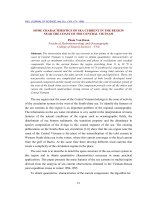
In order to obtain more accurate results of the above equations, we divide the pipeline to a
number of sections (ΔL), so that we can calculate the pressure drop (Δp) and value p at each
point more accurately (Fig. 1).












Figure 1. Gas pipeline arrangement scheme

Calculating pressure drop along pipeline is performed with the following steps:
1.
Starting with the known pressure, p
1
, at L
1

2.
Estimating a pressure increment Δp, corresponding to length ΔL.
3.

Calculating the average pressure and, for nonisothermal cases, the average temperature.
4.
From laboratory data or empirical correlations, determine the necessary fluid and p,V,T
properties at conditions of average pressure and temperature (ρ
g
υ
g
μ
g
).
5.
Calculating the pressure gradient dp/dL at average conditions of pressure, temperature,
and pipe inclination.
6.
Calculating the pressure increment corresponding to the selected section, Δp= ΔL(dp/dL).
7.
Comparing the estimated and calculated values of Δp obtained in steps 2 and 6, if they
are not sufficiently closed, using a new pressure increment and return to step 3. repeating steps
3 through 7 until the estimated and calculated values are sufficiently closed.
TẠP CHÍ PHÁT TRIỂN KH&CN, TẬP 9,Số 4-2006
Trang 17
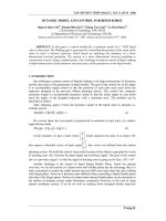
With this calculating order, establishing a program for pressure drop calculation along pipeline
will be done according to the scheme in Fig. 2.

No No

Yes Yes









Figure 2. Flow chart for calculating a pressure traverse
Read data
Be
g
in:
P
1
, L
1

i = 1
Evaluate ΔP
*

Re
p
eat = 0
set ΔL
Calc. PVT
Properties

),( PTf=
Cal. dp/dL &
Δp=ΔL(dp/dL)
ε
<Δ−Δ pp
*
Repeat >
limit
Repeat
= Re. + 1
Define Error Stop
Results
Stop
2/ppP
i
Δ±=

)(LfT =
)(Lf=
θ

Δp
*
=Δp
p = p
i
±Δp
Science & Technology Development, Vol 9, No.4 - 2006
Trang 18

The program calculating pressure drop along the associated gas pipeline is constructed in
Matlab environment, the software interface is introduced in Fig. 3.


Figure 3. Interface of pressure drop calculation in Matlab Environment

•
Result with data in table 3.1[6]:
Table 3.1. Input data
Description Sample 1 Sample 2 Sample 3
Inlet Temperature (
0
C) 42 45 46
Inlet gas pressure, (kPa) 10130 10860 120
Outlet Temperature (
0
C) 29 27 28
Outlet gas pressure, (kPa) 7730 7040 6970
Gas Flow, m
3
/day 3975600 5091360 6426480
Inlet gas compositions (mole fraction)
Compound
0.73037 0.75396 0.7380
Ethane (C
2
H
6
) 0.12989 0.12138 0.1219
Propane (C

3
H
8
) 0.07436 0.06905 0.073
i-Butane (C
4
H
10
) 0.016752 0.015021 0.0161
n-Butane (C
4
H
10
) 0.024459 0.021609 0.0234
i-Pentan (C
5
H
12
) 0.006284 0.005295 0.0061
n-Pentan (C
5
H
12
) 0.007038 0.005594 0.0068
Hexanes (C
6
H
14
) 0.004874 0.003584 0.0055
Heptanes (C

7
H
16
) 0.002331 0.001664 0.0032
Octan-plus (C
8
H
18
) 0.000711 0.000517 0.0012
Nonanes (C
9
H
20
) 0.000313 0.000257 0.0004
Decanes (C
10
H
22
) 0.00008 0.000079 0.0001
Nitro (N
2
) 0.00168 0.00151 0.0032
Dioxide carbone (CO
2
) 0.00087 0.00049 0.0011
Sulfide (H
2
S), ppm 9 9 10
Water (H
2

O), g/m
3
0.111 0.12 0.115
TẠP CHÍ PHÁT TRIỂN KH&CN, TẬP 9,Số 4-2006
Trang 19
The results with input data-sample 1 in table 3.1 along the associated gas pipeline of flow
equations of Weymouth, Panhandle A, Panhandle B and Clinedinst are stored in table 3.2a and
3.2b.
Table 3.2a. Pressure along associated gas pipeline with input data - sample 1 from table 3.1
Method
Weymouth Panhandle A

Location
along
pipeline
(m)
Pressure,
kPa
Coeff. of
Compressibility
– Z
Friction
Coeff.
Pressure,
KPa
Coeff. of
Compressibility
– Z
Friction
Coeff.

0 10130 10130
71 10128 0.7577 0.01301 10129 0.7575 0.00812
339 10120 0.7577 0.01301 10125 0.7519 0.00812
25071 9431 0.7577 0.0129 9812 0.7359 0.00814
52071 8630 0.7577 0.0129 9467 0.7256 0.00813
73071 7951 0.7577 0.0129 9193 0.7319 0.00810
105771 6760 0.7577 0.0129 8742 0.7398 0.00807
112971
6433
0.7577 0.01301
8628
0.7462 0.00803
Average 0.7577 0.01295 0.7413 0.00890
Real Pressure at 112971m of the end of pipeline is 7730 kPa
Table 3.2b.Pressure along associated gas pipeline with input data – sample 1 from table 3.1
Method
Panhandle B Clinedinst

Location
along
pipeline
(m)
Press
ure,
kPa
Coeff. of
Compressibility
– Z
Friction
Coeff.

Pressure,
KPa
Coeff. of
Compressibility
- Z
Friction
Coeff.
0 10130 10130
71 10129 0.7577 0.00799 10128 0.7578 0.01240
339 10125 0.7519 0.00799 10122 0.7520 0.01240
25071 9818 0.7359 0.00799 9640 0.7394 0.01235
52071 9482 0.7254 0.00799 9098 0.7336 0.01235
73071 9210 0.7317 0.00799 8647 0.7440 0.01235
105771 8765 0.7393 0.00798 7877 0.7597 0.01235
112971
8651
0.7457 0.00796
7673
0.7692 0.01234
Average 0.7411 0.00798 0.7508 0.01236
Real Pressure at 112971m of the end of pipeline is 7730 kPa

The results with input data - sample 2 in table 3.1 along the associated gas pipeline of flow
equations of Weymouth, Panhandle A, Panhandle B and Clinedinst are stored in table 3.3a and
3.3b.
Table 3.3a. Pressure along associated gas pipeline with input data – sample 2 from table 3.1

Method
Weymouth Panhandle A

Location
along
pipeline
(m)
Pressure,
kPa
Coeff. of
Compressibility
– Z
Frictio
n
Coeff.
Pressur
e,
KPa
Coeff. of
Compressibility
- Z
Friction
Coeff.
Science & Technology Development, Vol 9, No.4 - 2006
Trang 20
0 10860 10860
71 10857 0.7694 0.0130
1
10858 0.7706 0.007878
339 10844 0.7692 0.0130
1
10852 0.7623 0.007882
25071 9771 0.7692 0.0129

2
10383 0.7479 0.00790
52071 8498 0.7692 0.0129
2
9869 0.7337 0.007883
73071 7357 0.7692 0.0129
2
9447 0.7422 0.007851
105771 5094 0.7692 0.0129
2
8742 0.7532 0.007812
112971
4360
0.7692 0.0130
1
8560
0.7626 0.007763
Average 0.7692 0.0130 0.7532 0.00785
Real Pressure at 112971m of the end of pipeline is 7040 kPa
Table 3.3b. Pressure along associated gas pipeline with input data – sample 2 from table 3.1

Method
Panhandle B Clinedinst

Location
along
pipeline
(m)
Pressure,
kPa

Coeff. Of
Compressibility –
Z
Friction
Coeff.
Pressur
e,
KPa
Coeff. Of
Compressibi
lity – Z
Frictio
n
Coeff.
0 10860 10860
71 10858 0.7733 0.00792 10858 0.7706 0.0124
339 10853 0.7679 0.00792 10849 0.7623 0.0124
25071 10382 0.7479 0.00793 10107 0.7492 0.0123
52071 9865 0.7337 0.00792 9252 0.7450 0.0123
73071 9439 0.7422 0.00791 8512 0.7606 0.0123
105771 8724 0.7534 0.00790 7162 0.7862 0.0123
112971
8538
0.7630 0.00789
6781
0.8037 0.0124
Average 0.7530 0.00791 0.7682 0.0123
4
Real Pressure at 112971m of the end of pipeline is 7040 kPa
The results with input data - sample 3 in table 3.1 along the associated gas pipeline of flow

equations of Weymouth, Panhandle A, Panhandle B and Clinedinst are stored in table 3.4a and
3.4b.
Table 3.4a. Pressure along associated gas pipeline with input data – sample 3 from table 3.1
Method
Panhandle B Clinedinst

Location
along
pipeline
(m)
Pressure,
kPa
Coeff. Of
Compressibilit
y – Z
Friction
Coeff.
Pressure,
KPa
Coeff. Of
Compressibility
– Z
Friction
Coeff.
0 12000 12000
TẠP CHÍ PHÁT TRIỂN KH&CN, TẬP 9,Số 4-2006
Trang 21
71 11995 0.8037 0.01301 11998 0.7498 0.0076
6
339 11977 0.8037 0.01301 11990 0.7440 0.0076

6
25071 10402 0.8037 0.0129 11341 0.7224 0.0076
9
52071 8400 0.8037 0.0129 10622 0.7075 0.0076
7
73071 6425 0.8037 0.0129 10021 0.7181 0.0074
2
105771 8992 0.7332 0.0075
6
112971


8719
0.7471 0.0075
0
Trung
bình
0.8037 0.01294 0.7317 0.0075
94
Real Pressure at 112971m of the end of pipeline is 6970 kPa
Table 3.4b. Pressure along associated gas pipeline with input data – sample 3 from table 3.1
Method
Panhandle B Clinedinst

Location
along
pipeline
(m)
Pressure,
kPa

Coeff. Of
Compressibility
– Z
Friction
Coeff.
Pressure,
KPa
Coeff. Of
Compressibi
lity – Z
Friction
Coeff.
0 12000 12000
71 11998 0.7498 0.00786 11997 0.7499 0.01239
339 11989 0.7440 0.00786 11984 0.7441 0.01239
25071 11325 0.7224 0.00787 10914 0.7280 0.01234
52071 10585 0.7079 0.00786 9648 0.7239 0.01233
73071 9963 0.7189 0.00785 8497 0.7474 0.01234
105771 8885 0.7348 0.00783 6137 0.7935 0.01233
112971
8596
0.7496 0.00781
5367
0.7296 0.01234
Trung
bình

0.7325 0.00785 0.7452 0.01235
Real Pressure at 112971m of the end of pipeline is 6970 kPa
Table 3.5. Summary of numerical results of oulet pressure p

2

Results of outlet pressure and its differences with the real value
Input data
Table 3.2,
(samp. 1)
Input data
Table 3.3,
(samp. 2)
Input data
Table 3.4,
(samp. 3)


Method
Pressure,
kPa
% diff. Pressure,
kPa
% diff. Pressure,
kPa
% diff.
Weymouth 6433 16.8 4360 38.1 -(*) -
Panhandle A 8628 -11.6 8560 -21.6 8719 -25.1
Panhandle B 8651 -11.9 8538 21.3 8596 23.3
Clinedinst 7673 0.7 6781 3.7 5367 23.0
(*) Pressure –p
2
is not converged
Science & Technology Development, Vol 9, No.4 - 2006

Trang 22
Summarization of the numerical results for output pressure is listed in Table 3.5. From the
results, it is clear that:
-
None of those calculations gives the same result as practical data, but the result is
acceptable when we combine all the one-phase flow equations of Weymouth, Panhandle A,
Panhandle B and Clinedinst in calculating pressure drop along the associated gas pipeline.
-
The first group of input data gives the most suitable results in comparison with measured
values.
-
Coefficient of compressibility Z in different calculating methods doesn’t vary much, but
friction coefficient does. It proves that, friction coefficient is the key cause of different results.
4. CONCLUSION
From the research, it is believed that, the combination of all the flow equations of
Weymouth, Panhandle A, Panhandle B and Clinedinst in calculating pressure drop along the
associated gas pipeline is very helpful to establish the mutual relationship between technical
statistics. Friction coefficient is the main cause of different results in calculation. This brings
about a need to determine a new correlation for friction coefficient to make it suitable for the
associated gas pipeline in practice. The authors are very gracious to the Basic Studies Fund of
Natural Science Committee from which our works receives precious support.
MÔ HÌNH SỐ DÒNG MỘT PHA TRONG TÍNH TOÁN TỔN THẤT ÁP SUẤT
DỌC ĐƯỜNG ỐNG DẪN KHÍ
Vũ Tú Hoài
(1)
, Nguyễn Thanh Nam
(2)
(1) J. V. “Vietsovpetro”
(2) Trường Đại học Bách khoa, ĐHQG-HCM
TÓM TẮT: Để công việc vận chuyển dầu khí an toàn và hiệu quả, điều cần phải quan

tâm đầu tiên đó là tính toán suy giảm áp lực dọc theo tuyến ống dẫn khí. Nếu chúng ta không
tính suy giảm áp lực dọc theo tuyến ống dẫn khí thì sẽ không thể kiểm soát được qúa trình vận
chuyển. Trong thực tế việc tính toán chính xác các thông số từ các phương trình dòng chảy là
rất khó thực hiện vì chúng liên quan tới nhiều qúa trình hóa lý và diễn biến động học phứ
c tạp.
Do vậy, một số phương trình thực nghiệm có nguồn gốc từ phương trình dòng và các đại lượng
vật lý liên quan đã được sử dụng để tính suy giảm áp lực dọc theo tuyến ống dẫn khí. Kết qủa
tính cho từng trường hợp được kiểm tra lại với số liệu của đường ống thực tế. Từ đó rút ra
phương pháp tính phù hợp nhất áp dụng cho tuyến
ống dẫn khí từ mỏ Bạch hổ về trạm Dinh cố.
REFERENCES
[1]. John M.Campbell, Gas Conditioning and Processing, Vol. 2 The Equipment Modules,
chapter 10, Prented and Bound in USA, October 1994.
[2].
Robert N. Maddox & Larry I. Lilly, Gas Conditioning and Processing, Vol. 3 Computer
Applications & Production/Processing Facilities, Prented and Bound in USA, October
1994.
[3].
Clement Kleinstreuer, Flow-Theory and Applications, Taylor & Francis, 2003.
[4].
Sanjay Kumar, Gas Production Engineering, Gulf Publishing Company, p.p 275-292,
1960.
TẠP CHÍ PHÁT TRIỂN KH&CN, TẬP 9,Số 4-2006
Trang 23
[5]. Tulsa, Oklahoma, Gas Processors Suppliers Association, Engineering Data Book,
Volume I & II, 1998.
[6].
Vũ Tú Hoài, Nghiên cứu, tính toán công nghệ vận chuyển khí đồng hành từ mỏ Bạch hổ
về bờ, MSc. Thesis, HCMUT, 2005.