Networking Theory and Fundamentals - Lecture 6 pot
Bạn đang xem bản rút gọn của tài liệu. Xem và tải ngay bản đầy đủ của tài liệu tại đây (343.64 KB, 33 trang )
1
TCOM 501:
Networking Theory & Fundamentals
Lecture 6
February 19, 2003
Prof. Yannis A. Korilis
6-2
Topics
Time-Reversal of Markov Chains
Reversibility
Truncating a Reversible Markov Chain
Burke’s Theorem
Queues in Tandem
6-3
Time-Reversed Markov Chains
{X
n
: n=0,1,…} irreducible aperiodic Markov chain with
transition probabilities P
ij
Unique stationary distribution (π
j
> 0) if and only if:
Process in steady state:
Starts at n=-∞, that is {X
n
: n = …,-1,0,1,…}
Choose initial state according to the stationary distribution
How does {X
n
} look “reversed” in time?
0
ππ,0,1,
jiij
i
Pj
∞
=
==
∑
0
1, 0,1,
ij
j
Pi
∞
=
==
∑
0
Pr{ } lim Pr |π {}
n
n
nj
XXX ij j
→∞
=
==
=
=
6-4
Time-Reversed Markov Chains
Define Y
n
=X
τ-n
, for arbitrary τ>0
{Y
n
} is the reversed process.
Proposition 1:
{Y
n
} is a Markov chain with transition probabilities:
{Y
n
} has the same stationary distribution π
j
with the
forward chain {X
n
}
*
π
,, 0,1,
π
jji
ij
i
P
Pij==
6-5
Time-Reversed Markov Chains
Proof of Proposition 1:
*
122
122
122
122
122
22
{| , ,, }
{| , ,, }
{| , ,, }
{, , ,, }
{, ,, }
{,, |,
ij m m m m k k
mm m mkk
nn n nkk
nn n nkk
nn nkk
nnkknn
PPY jY iY i Y i
PX j X iX i X i
PX j X iX i X i
PX jX iX i X i
PX iX i X i
PX i X i X jX
ττ τ τ
−− −
−−+−+ −+
++ +
++ +
++ +
++ +
== = = =
== = = =
== = = =
=== =
=
== =
===
=
…
…
…
…
…
…
11
22 1 1
1
1
1
1
11
}{ , }
{,, |}{}
{, }
{}
π
{|}{}
{| } |}
{} π
{
nn
nnkknn
nn
nn m
n
ji j
n
m
nn
ni
iPX jX i
PX i X
PX j X i PY
iX iPX i
PX jX i
PX i
P
PX i X jP
j
X
Yi
j
PX i
+
++++
+
+
+
+
+
−
=
==
====
==
==
=
== =
==
=
== = =
=
…
*
00 0
π
πππ π
π
jji
iij i j ji j
ii i
i
P
PP
∞∞ ∞
== =
===
∑∑ ∑
6-6
Reversibility
Stochastic process {X(t)} is called reversible if
(X(t
1
), X(t
2
),…, X(t
n
)) and (X(τ-t
1
), X(τ-t
2
),…, X(τ-t
n
))
have the same probability distribution, for all τ, t
1
,…, t
n
Markov chain {X
n
} is reversible if and only if the transition
probabilities of forward and reversed chains are equal
or equivalently, if and only if
Detailed Balance Equations ↔ Reversibility
*
ij ij
PP
=
ππ, , 0,1,
iij j ji
PPij
=
=
6-7
Reversibility – Discrete-Time Chains
Theorem 1: If there exists a set of positive numbers {π
j
}, that
sum up to 1 and satisfy:
Then:
1. {π
j
} is the unique stationary distribution
2. The Markov chain is reversible
Example: Discrete-time birth-death processes are reversible,
since they satisfy the DBE
ππ, , 0,1,
iij j ji
PPij
=
=
6-8
Example: Birth-Death Process
One-dimensional Markov chain with transitions only
between neighboring states:
P
ij
=0, if |i-j|>1
Detailed Balance Equations (DBE)
Proof: GBE with S ={0,1,…,n} give:
0 1 n+1n2
,1nn
P
+
1,nn
P
+
,nn
P
,1nn
P
−
1,nn
P
−
01
P
10
P
00
P
SS
c
,1 1 1,
ππ 0,1,
nnn n n n
PPn
+++
=
=
,1 1 1,
01 01
ππππ
nn
jji iij nnn n n n
jin jin
P
PP P
∞∞
+++
==+ ==+
=⇒=
∑∑ ∑∑
6-9
Time-Reversed Markov Chains (Revisited)
Theorem 2: Irreducible Markov chain with transition probabilities P
ij.
If
there exist:
A set of transition probabilities Q
ij
, with ∑
j
Q
ij
=1, i ≥ 0, and
A set of positive numbers {π
j
}, that sum up to 1, such that
Then:
Q
ij
are the transition probabilities of the reversed chain, and
{π
j
} is the stationary distribution of the forward and the reversed chains
Remark: Use to find the stationary distribution, by guessing the transition
probabilities of the reversed chain – even if the process is not reversible
ππ,,0,1, (1)
iij j ji
PQij
=
=
6-10
Continuous-Time Markov Chains
{X(t): -∞< t <∞} irreducible aperiodic Markov chain with
transition rates q
ij
, i≠j
Unique stationary distribution (p
i
> 0) if and only if:
Process in steady state – e.g., started at t =-∞:
If {π
j
}, is the stationary distribution of the embedded
discrete-time chain:
, 0,1,
jji iij
ij ij
pq pqj
≠≠
==
∑
∑
limPr{ ( ) Pr{ ( ) | (0)} }
t
j
XXt tXp
j
ij
→∞
=
==
=
=
π /
, , 0,1,
π /
jj
jjji
ij
ii
i
pqj
ν
ν
ν
≠
=≡=
∑
∑
6-11
Reversed Continuous-Time Markov Chains
Reversed chain {Y(t)}, with Y(t)=X(τ-t), for arbitrary τ>0
Proposition 2:
1. {Y(t)} is a continuous-time Markov chain with transition rates:
2. {Y(t)} has the same stationary distribution {p
j
} with the forward chain
Remark: The transition rate out of state i in the reversed chain is equal
to the transition rate out of state i in the forward chain
*
, , 0,1, ,
jji
ij
i
pq
qijij
p
=
=≠
*
, 0,1,
jji i ij
ji ji
ij ij i
ji ji
ii
pq p q
qqi
pp
ν
≠≠
≠≠
=====
∑
∑
∑∑
6-12
Reversibility – Continuous-Time Chains
Markov chain {X(t)} is reversible if and only if the transition rates of
forward and reversed chains are equal or equivalently
Detailed Balance Equations ↔ Reversibility
Theorem 3: If there exists a set of positive numbers {p
j
}, that sum up to 1
and satisfy:
Then:
1. {p
j
} is the unique stationary distribution
2. The Markov chain is reversible
*
,
ij ij
qq=
, , 0,1, ,
iij j ji
pq p q i
j
i
j
=
=≠
, , 0,1, ,
iij j ji
pq p q i
j
i
j
=
=≠
6-13
Example: Birth-Death Process
Transitions only between neighboring states
Detailed Balance Equations
Proof: GBE with S ={0,1,…,n} give:
M/M/1, M/M/c, M/M/∞
0 1 n+1n2
0
λ
1
µ
n
λ
1n
µ
+
1
λ
2
µ
1n
λ
−
n
µ
,1 ,1
,,0,||1
ii i ii i ij
qqqij
λ
µ
+−
===−>
11
, 0,1,
nn n n
ppn
λ
µ
++
=
=
11
01 01
nn
j
ji i ij n n n n
jin jin
p
qpqpp
λµ
∞∞
+
+
==+ ==+
=⇒=
∑∑ ∑∑
SS
c
6-14
Reversed Continuous-Time Markov Chains (Revisited)
Theorem 4: Irreducible continuous-time Markov chain with transition rates
q
ij.
If there exist:
A set of transition rates φ
ij
, with ∑
j≠i
φ
ij
=∑
j≠i
q
ij
, i ≥ 0, and
A set of positive numbers {p
j
}, that sum up to 1, such that
Then:
φ
ij
are the transition rates of the reversed chain, and
{p
j
} is the stationary distribution of the forward and the reversed chains
Remark: Use to find the stationary distribution, by guessing the transition
probabilities of the reversed chain – even if the process is not reversible
, , 0,1, ,
iij j ji
ppqi
j
i
j
ϕ
=
=≠
6-15
Reversibility: Trees
Theorem 5:
For a Markov chain form a graph, where states are the nodes, and for
each q
ij
>0, there is a directed arc i→j
Irreducible Markov chain, with transition rates that satisfy q
ij
>0 ↔ q
ji
>0
If graph is a tree – contains no loops – then Markov chain is reversible
Remarks:
Sufficient condition for reversibility
Generalization of one-dimensional birth-death process
01
q
0 1
2
6
3
7
4
5
10
q
12
q
21
q
16
q
61
q
23
q
32
q
67
q
76
q
6-16
Kolmogorov’s Criterion (Discrete Chain)
Detailed balance equations determine whether a Markov chain is
reversible or not, based on stationary distribution and transition
probabilities
Should be able to derive a reversibility criterion based only on the
transition probabilities!
Theorem 6: A discrete-time Markov chain is reversible if and only if:
for any finite sequence of states: i
1
, i
2
,…, i
n
, and any n
Intuition: Probability of traversing any loop i
1
→i
2
→…→i
n
→i
1
is equal
to the probability of traversing the same loop in the reverse direction
i
1
→i
n
→…→i
2
→i
1
12 23 1 1 1 1 32 21nn n n nn
ii i i i i i i ii i i ii i i
P
PPPPP PP
−−
=
6-17
Kolmogorov’s Criterion (Continuous Chain)
Detailed balance equations determine whether a Markov chain is
reversible or not, based on stationary distribution and transition rates
Should be able to derive a reversibility criterion based only on the
transition rates!
Theorem 7: A continuous-time Markov chain is reversible if and only if:
for any finite sequence of states: i
1
, i
2
,…, i
n
, and any n
Intuition: Product of transition rates along any loop i
1
→i
2
→…→i
n
→i
1
is equal to the product of transition rates along the same loop traversed
in the reverse direction i
1
→i
n
→…→i
2
→i
1
12 23 1 1 1 1 32 21nn n n nn
ii i i i i i i ii i i ii i i
qq q q qq qq
−−
=
6-18
Kolmogorov’s Criterion (proof)
Proof of Theorem 6:
Necessary: If the chain is reversible the DBE hold
Sufficient: Fixing two states i
1
=i, and i
n
=j and summing over all states
i
2
,…, i
n-1
we have
Taking the limit n→∞
12 21
23 32
12 23 1 1 1 1 32 21
11
11
12
23
1
1
ππ
ππ
ππ
ππ
nn n n nn
nn nn
nn
ii i i
ii ii
ii ii i i ii ii ii ii ii
nii nii
nii ii
PP
PP
P
PPPPP PP
PP
PP
−−
−−
−
=
=
⇒=
=
=
223 1 1 322
11
,,,,
nn
nn
i i i i i j ji ij j i i i i i ij ji ij ji
P
PPPPP PP PPPP
−−
−−
=⇒=
11
lim lim ππ
nn
i
jj
ii
jj
i
jj
ii
j
i
nn
P
PP P PP
−−
→∞ →∞
⋅=⋅ ⇒ =
6-19
Example: M/M/2 Queue with Heterogeneous Servers
α
λ
λ
λ
λ
0
1A
1B
(1 )
α
λ
−
A
µ
B
µ
2
3
λ
B
µ
A
µ
AB
µ
µ
+
AB
µ
µ
+
M/M/2 queue. Servers A and B with service rates µ
A
and µ
B
respectively.
When the system empty, arrivals go to A with probability α and to B with
probability 1-α. Otherwise, the head of the queue takes the first free server.
Need to keep track of which server is busy when there is 1 customer in the
system. Denote the two possible states by: 1A and 1B.
Reversibility: we only need to check the loop 0→1A→2→1B→0:
Reversible if and only if α=1/2.
What happens when µ
A
=µ
B
, and α≠1/2?
0,1 1 ,2 2,1 1 ,0 0,1 1 ,2 2,1 1 ,0
(1 )
A
ABB AB BBAA BA
qqqq qqqq
α
λλµ µ αλλµ µ
=
⋅⋅ ⋅ = − ⋅⋅ ⋅
6-20
Example: M/M/2 Queue with Heterogeneous Servers
α
λ
λ
λ
λ
0
1A
1B
(1 )
α
λ
−
A
µ
B
µ
2
3
λ
B
µ
A
µ
AB
µ
µ
+
AB
µ
µ
+
S
3
S
2
S
1
2
2
, 2,3,
n
n
AB
pp n
λ
µµ
−
==
+
10
01 1
211 10
102
2
20
()
2
(1 )( )
()( )
2
()
(1 )
2
AB
A
AAB
AA BB
AB
AB A B B
BAB
AA B
A
B
AB A B
pp
pp p
ppp pp
ppp
pp
λ
λαµ µ
µλµµ
λµ µ
λλ α µ µ
µµ λ
µλµµ
µλ αλ µ
λ
λαµαµ
µµ λ µ µ
+
+
=
++
=+
+− +
+=+ ⇒=
++
+=+
+− +
=
++
1
2
01 1 0
2
(1 )
11
2
AB
AB n
n
AB AB AB
pp p p p
−
∞
=
+− +
+++ =⇒=+
+− ++
∑
λλλαµαµ
µµλµµ λµµ
6-21
Multidimensional Markov Chains
Theorem 8:
{X
1
(t)}, {X
2
(t)}: independent Markov chains
{X
i
(t)}: reversible
{X(t)}, with X(t)=(X
1
(t), X
2
(t)): vector-valued stochastic process
{X(t)} is a Markov chain
{X(t)} is reversible
Multidimensional Chains:
Queueing system with two classes of customers, each having its own
stochastic properties – track the number of customers from each class
Study the “joint” evolution of two queueing systems – track the number
of customers in each system
6-22
Example: Two Independent M/M/1 Queues
Two independent M/M/1 queues. The arrival and service rates at queue i
are λ
i
and µ
i
respectively. Assume ρ
i
= λ
i
/µ
i
<1.
{(N
1
(t), N
2
(t))} is a Markov chain.
Probability of n
1
customers at queue 1, and n
2
at queue 2, at steady-state
“Product-form” distribution
Generalizes for any number K of independent queues, M/M/1, M/M/c,
or M/M/∞. If p
i
(n
i
) is the stationary distribution of queue i:
12
12 1 1 2 2 11 22
(, ) (1 ) (1 ) () ()
nn
p
nn pn p n
ρρ ρρ
=− ⋅− = ⋅
12 11 22
(, , , ) () () ( )
KKK
p
nn n pn p n p n
=
……
6-23
Example: Two Independent M/M/1 Queues
Stationary distribution:
Detailed Balance Equations:
Verify that the Markov chain is
reversible – Kolmogorov criterion
12
11 2 2
12
11 2 2
(, ) 1 1
nn
pn n
λλ λλ
µµ µµ
=− −
11 2 112
212 212
(1,) (,)
(, 1) (, )
pn n pn n
pn n pn n
µ
λ
µλ
+=
+=
2
λ
2
µ
2
λ
2
µ
2
λ
2
µ
2
λ
2
µ
2
λ
2
µ
2
λ
2
µ
2
λ
2
µ
2
λ
2
µ
2
λ
2
µ
2
λ
2
µ
2
λ
2
µ
2
λ
2
µ
02 12
22
32
1
λ
1
λ
1
λ
1
µ
1
µ
1
µ
01 11
21
31
1
λ
1
λ
1
λ
1
µ
1
µ
1
µ
00 10
20 30
1
λ
1
λ
1
λ
1
µ
1
µ
1
µ
03 13
23
33
1
λ
1
λ
1
λ
1
µ
1
µ
1
µ
6-24
Truncation of a Reversible Markov Chain
Theorem 9: {X(t)} reversible Markov process with state space S, and
stationary distribution {p
j
: j∈S}. Truncated to a set E⊂S, such that the
resulting chain {Y(t)} is irreducible. Then, {Y(t)} is reversible and has
stationary distribution:
Remark: This is the conditional probability that, in steady-state, the
original process is at state j, given that it is somewhere in E
Proof: Verify that:
,
j
j
k
kE
p
pj
E
p
∈
=
∈
∑
,, ;
1
j
i
j ji i ij ji ij j ji i ij
kk
kE kE
j
j
jE jE
k
kE
p
p
p q pq q q p q pq i j S i j
pp
p
p
p
∈∈
∈∈
∈
=⇔ = ⇔ = ∈≠
==
∑∑
∑∑
∑
6-25
Example: Two Queues with Joint Buffer
The two independent M/M/1 queues of
the previous example share a common
buffer of size B – arrival that finds B
customers waiting is blocked
State space restricted to
Distribution of truncated chain:
Normalizing:
Theorem specifies joint distribution up
to the normalization constant
0 Calculation of normalization constant is
often tedious
2
λ
2
µ
2
λ
2
µ
2
λ
2
µ
1
λ
1
µ
2
λ
2
µ
2
λ
2
µ
2
λ
2
µ
1
λ
1
µ
1
λ
1
µ
1
λ
1
µ
2
λ
2
µ
2
λ
2
µ
2
λ
2
µ
02 12
1
λ
1
µ
01 11
21
1
λ
1
λ
1
µ
1
µ
00 10
20 30
1
λ
1
λ
1
µ
1
µ
03 13
22
31
12 1 2
{( , ) :( 1) ( 1) }Ennn n B
++
=−+−≤
12
12 1 2 12
(, ) (0,0) ,(, )
nn
pn n p n n E
ρρ
=⋅ ∈
12
12
1
12
(,)
(0,0)
nn
nn E
p
ρρ
−
∈
=
∑
State diagram for B =2