Basic Theory of Plates and Elastic Stability - Part 5 pptx
Bạn đang xem bản rút gọn của tài liệu. Xem và tải ngay bản đầy đủ của tài liệu tại đây (658.25 KB, 85 trang )
Scawthorn, C. “Earthquake Engineering”
Structural Engineering Handbook
Ed. Chen Wai-Fah
Boca Raton: CRC Press LLC, 1999
Earthquake Engineering
Charles Scawthorn
EQE International, San Francisco,
California and Tokyo, Japan
5.1 Introduction
5.2 Earthquakes
Causes of Earthquakes and Faulting
•
Distribution of Seis-
micity
•
Measurement of Earthquakes
•
Strong Motion At-
tenuation and Duration
•
Seismic Hazard and Design Earth-
quake
•
Effect of Soils on Ground Motion
•
Liquefaction and
Liquefaction-Related Permanent Ground Displacement
5.3 Seismic Design Codes
Purpose of Codes
•
Historical Development of Seismic Codes
•
Selected Seismic Codes
5.4 Earthquake Effects and Design of Structures
Buildings
•
Non-Building Structures
5.5 Defining Terms
References
Further Reading
5.1 Introduction
Earthquakes are naturally occurring broad-banded vibratory ground motions, caused by a number
of phenomena including tectonic ground motions, volcanism, landslides, rockbursts, and human-
made explosions. Of these various causes, tectonic-related earthquakes are the largest and most
important. These are caused by the fracture and sliding of rock along faults within the Earth’s
crust. A fault is a zone of the earth’s crust within which the two sides have moved — faults may
be hundreds of miles long, from 1 to over 100 miles deep, and not readily apparent on the ground
surface. Earthquakes initiate a number of phenomena or agents, termed seismic hazards, which can
cause significant damage to the built environment — these include fault rupture, vibratory ground
motion (i.e., shaking), inundation (e.g., tsunami, seiche, dam failure), various kinds of permanent
ground failure (e.g., liquefaction), fire or hazardous materials release. For a given earthquake, any
particular hazard can dominate, and historically each has caused major damage and great loss of
life in specific earthquakes. The expected damage given a specified value of a hazard parameter is
termed vulnerability, and the product of the hazard and the vulnerability (i.e., the expected damage)
is termed the seismic risk. This is often formulated as
E(D) =
H
E(D | H)p(H)dHψ (5.1)
where
Hψ = hazard
p(·)ψ = refers to probability
Dψ = damage
c
1999 by CRC Press LLC
E(D|H) = vulnerability
E(·) = the expected value operator
Note that damage can refer to various parameters of interest, such as casualties, economic loss,
or temporal duration of disruption. It is the goal of the earthquake specialist to reduce seismic risk.
The probability of having a specific level of damage (i.e., p(D) = d)istermedthefragility.
For most earthquakes, shaking is the dominant and most widespread agent of damage. Shaking
near the actual earthquake rupture lasts only during the time when the fault ruptures, a process
that takes seconds or at most a few minutes. The seismic waves gener ated by the r upture propagate
long after the movement on the fault has stopped, however, spanning the globe in about 20 minutes.
Typically earthquake ground motions are powerful enough to cause damageonly in the near field (i.e.,
within a few tens of kilometers from the causative fault). However, in a few instances, long period
motions have caused significant damage at great distances to selected lightly damped structures. A
prime example of this was the 1985 Mexico City earthquake, where numerous collapses of mid- and
high-rise buildings were due to a Magnitude 8.1 earthquake occurring at a distance of approximately
400 km from Mexico City.
Ground motions due to an earthquake will vibrate the base of a structure such as a building.
These motions are, in general, three-dimensional, both lateral and vertical. The structure’s mass has
inertia which tends to remain at rest as the structure’s base is vibrated, resulting in deformation of
the structure. The structure’s load carrying members will try to restore the structure to its initial,
undeformed, configuration. As the structure rapidly deforms, energy is absorbed in the process of
material deformation. These characteristics can be effectively modeled for a single degree of freedom
(SDOF) mass as shown in Figure 5.1 where m represents the mass of the structure, the elastic spring
(of stiffness k =force /displacement) represents the restorative force of the structure, and the dashpot
damping device (damping coefficient c = force/velocity) represents the force or energy lost in the
process of material deformation. From the equilibrium of forces on mass m due to the spring and
FIGURE 5.1: Single degree of freedom (SDOF) system.
dashpot damper and an applied load p(t), we find:
m ¨u + c ˙u + ku = p(t)
(5.2)
the solution of which [32] provides relations between circular frequency of vibration ω, the natural
frequency f , and the natural period T :
2
=
k
m
(5.3)
f =
1
T
=
2π
=
1
2π
k
m
(5.4)
c
1999 by CRC Press LLC
Damping tends to reduce the amplitude of vibrations. Critical damping referstothevalueof
damping such that free vibration of a structure will cease after one cycle (c
crit
= 2mω). Damping is
conventionally expressed as a percent of critical damping and, for most buildings and engineering
structures, ranges from 0.5 to10or20% of critical damping (increasing with displacementamplitude).
Note thatdampinginthisrange will not appreciablyaffectthenaturalperiodorfrequency of vibration,
but does affect the amplitude of motion experienced.
5.2 Earthquakes
5.2.1 Causes of Earthquakes and Faulting
In a global sense, tectonic earthquakes result from motion between a number of large plates com-
prising the earth’s crust or lithosphere (about 15 in total), (see Figure 5.2). These plates are driven
by the convective motion of the mater ial in the earth’s mantle, which in turn is driven by heat gener-
ated at the earth’s core. Relative plate motion at the fault interface is constrained by friction and/or
asperities (areas of interlocking due to protrusions in the fault surfaces). However, strain energ y
accumulates in the plates, eventually overcomes any resistance, and causes slip between the two sides
of the fault. This sudden slip, termed elastic rebound by Reid [101] based on his studies of regional
deformation following the 1906 San Francisco earthquake, releases large amounts of energy, which
constitutes the earthquake. The location of initial radiation of seismic waves (i.e., the first location of
dynamic rupture) is termed the hypocenter, while the projection on the surface of the earth directly
above the hypocenter is termed the epicenter. Other terminology includes near-field (within one
source dimension of the epicenter, where source dimension refers to the length or width of faulting,
whichever is less), far-field (beyond near-field), and meizoseismal (the area of strong shaking and
damage). Energy is radiated over a broad spectrum of frequencies through the earth, in body waves
and surface waves [16]. Body waves are of two types: P waves (transmitting energy via push-pull
motion), and slower S waves (transmitting energy via shear action at right angles to the direction of
motion). Surface waves are also of two types: horizontally oscillating Love waves (analogous to S
body waves) and vertically oscillating Rayleigh waves.
While the accumulation of strain energy within the plate can cause motion (and consequent release
of energy) at faults at any location, earthquakes occur with greatest frequency at the boundaries of
the tectonic plates. The boundary of the Pacific plate is the source of nearly half of the world’s great
earthquakes. Stretching 40,000 km (24,000 miles) around the circumference of the Pacific Ocean,
it includes Japan, the west coast of North America, and other highly populated areas, and is aptly
termed the Ring of Fire. The interiors of plates, such as ocean basins and continental shields, are areas
of low seismicity but are not inactive — the largest earthquakes known to have occurred in North
America, for example, occurred in the New Madrid area, far from a plate boundary. Tectonic plates
move very slowly and irregularly, with occasional earthquakes. Forces may build up for decades or
centuries at plate interfaces until a large movement occurs all at once. These sudden, violent motions
produce the shaking that is felt as an earthquake. The shaking can cause direct damage to building s,
roads, bridges, and other human-made structures as well as triggering fires, landslides, tidal waves
(tsunamis), and other damaging phenomena.
Faults are the physical expression of the boundaries between adjacent tectonic plates and thus
may be hundreds of miles long. In addition, there may be thousands of shorter faults parallel to
or branching out from a main fault zone. Generally, the longer a fault the larger the earthquake
it can generate. Beyond the main tectonic plates, there are many smaller sub-plates (“platelets”)
and simple blocks of crust that occasionally move and shift due to the “jostling” of their neighbors
and/or the major plates. The existence of these many sub-plates means that smaller but still damaging
earthquakes are possible almost anywhere, although often with less likelihood.
c
1999 by CRC Press LLC
FIGURE 5.2: Global seismicity and major tectonic plate boundaries.
c
1999 by CRC Press LLC
Faults are typically classified according to their sense of motion (Figure 5.3). Basic terms include
FIGURE 5.3: Fault types.
transform or strike slip (relative fault motion occurs in the horizontal plane, parallel to the strike of
the fault), dip-slip (motion at right angles to the strike, up- or down-slip), normal (dip-slip motion,
two sides in tension, move away from each other), reverse (dip-slip, two sides in compression, move
towards each other), and thrust (low-angle reverse faulting).
Generally, earthquakes will be concentrated in the vicinity of faults. Faults that are moving more
rapidly than others will tend to have higher rates of seismicity, and larger faults are more likely
than others to produce a large event. Many faults are identified on regional geological maps, and
useful information on fault location and displacement history is available from local and national
geological sur veys in areas of high seismicity. Considering this information, areas of an expected
large earthquake in the near future (usually measured in years or decades) can be and have been
identified. However, earthquakes continue to occur on “unknown” or “inactive” faults. An important
development has been the growing recognition of blind thrust faults, which emerged as a result of
several earthquakes in the 1980s, none of which were accompanied by surface faulting [120]. Blind
thrust faults are faults at depth occurring under anticlinal folds — since they have only subtle surface
expression, their seismogenic potential can be evaluated by indirect means only [46]. Blind thrust
faults are particularly worrisome because they are hidden, are associated with folded topography in
general, including areas of lower and infrequent seismicity, and therefore result in a situation where
the potential for an earthquake exists in any area of anticlinal geology, even if there are few or no
earthquakes in the historic record. Recent major earthquakes of this type have included the 1980 M
w
7.3 El- Asnam (Algeria), 1988 M
w
6.8 Spitak (Armenia), and 1994 M
w
6.7 Northridge (California)
events.
Probabilistic methods can be usefully employed to quantify the likelihood of an earthquake’s
occurrence, and typically form the basis for determining the design basis earthquake. However, the
earthquake generating process is not understood well enough to reliably predict the times, sizes, and
c
1999 by CRC Press LLC
locations of earthquakes with precision. In general, therefore, communities must be prepared for an
earthquake to occur at any time.
5.2.2 Distribution of Seismicity
This section discusses and characterizes the distr ibution of seismicity for the U.S. and selected areas.
Global
It is evident from Figure 5.2that some parts ofthe globe experience more and larger earthquakes
than others. The two major regions of seismicity are the circum-Pacific Ring of Fire and the Tr ans-
Alpide belt, extending from the western Mediterranean through the Middle East and the northern
India sub-continent to Indonesia. The Pacific plate is created at itsSouth Pacific extensional boundary
— its motion is generally northwestward, resulting in relative strike-slip motion in California and
New Zealand (with, however, a compressive component), and major compression and subduction
in Alaska, the Aleutians, Kuriles, and northern Japan. Subduction refers to the plunging of one plate
(i.e., the Pacific) beneath another, into the mantle, due to convergent motion, as shown in Figure 5.4.
FIGURE 5.4: Schematic diagram of subduction zone, typical of west coast of South America, Pacific
Northwest of U.S., or Japan.
Subduction zones are typically characterized by volcanism, as a portion of the plate (melting in
the lower mantle) re-emerges as volcanic lava. Subduction also occurs along the west coast of South
America at the boundary of the Nazca and South American plate, in Central America (boundary of the
Cocos and Caribbean plates), in Taiwan and Japan (boundary of the Philippine and Eurasian plates),
and in the North American Pacific Northwest (boundary of the Juan de Fuca and North American
c
1999 by CRC Press LLC
plates). The Trans-Alpide seismic belt is basically due to the relative motions of the African and
Australian plates colliding and subducting with the Eurasian plate.
U.S.
Table 5.1 provides a list of selected U.S. earthquakes. The San Andreas fault system in California
and the Aleutian Trench off the coast of Alaska are part of the boundary between the North American
and Pacific tectonic plates, and are associated with the majority of U.S. seismicity (Figure 5.5 and
Table 5.1). There are many other smaller fault zones throughout the western U.S. that are also helping
to release the stress that is built up as the tectonic plates move past one another, (Figure 5.6). While
California has had numerous destructive earthquakes, there is also clear evidence that the potential
exists for great earthquakes in the Pacific Northwest [11].
FIGURE 5.5: U.S. seismicity. (From Algermissen, S. T., An Introduction to the Seismicity of the United
States, Earthquake Engineering Research Institute, Oakland, CA, 1983. With permission. Also after
Coffman, J. L., von Hake, C. A., and Stover, C. W., Earthquake History of the United States, U.S.
Department of Commerce, NOAA, Pub. 41-1, Washington, 1980.)
On the east coast of the U.S., the cause of earthquakes is less well understood. There is no plate
boundary and very few locations of active faults are known so that it is more difficult to assess where
earthquakes are most likely to occur. Several significant historical earthquakes have occurred, such as
in Charleston, South Carolina, in 1886, and New Madrid, Missouri, in 1811 and 1812, indicating that
there is potential for very large and destructive earthquakes [56, 131]. However, most earthquakes in
the eastern U.S. are smaller magnitude events. Because of regional geologic differences, eastern and
central U.S. earthquakes are felt at much greater distances than those in the western U.S., sometimes
up to a thousand miles away [58].
c
1999 by CRC Press LLC
TABLE 5.1 Selected U.S. Earthquakes
USD
Yr M D Lat. Long. M MMI Fat. mills Locale
1755 11 18 8 Nr Cape Ann, MA
(MMI from STA)
1774 2 21 7 Eastern VA (MMI from STA)
1791 5 16 8 E. Haddam, CT
(MMI from STA)
1811 12 16 36 N 90 W 8.6 - New Madrid, MO
1812 1 23 36.6 N 89.6 W 8.4 12 New Madrid, MO
1812 2 7 36.6 N 89.6 W 8.7 12 New Madrid, MO
1817 10 5 8 Woburn, MA (MMI from STA)
1836 6 10 38 N 122 W - 10 - California
1838 6 0 37.5 N 123 W - 10 - California
1857 1 9 35 N 119 W 8.3 7 - San Francisco, CA
1865 10 8 37 N 122 W - 9 San Jose, Santa Cruz, CA
1868 4 3 19 N 156 W - 10 81 Hawaii
1868 10 21 37.5 N 122 W 6.8 10 3 Hayward, CA
1872 3 26 36.5 N 118 W 8.5 10 50 Owens Valley, CA
1886 9 1 32.9 N 80 W 7.7 9 60 5 Charleston, SC, Ms from STA
1892 2 24 31.5 N 117 W - 10 - San Diego County, CA
1892 4 19 38.5 N 123 W - 9 - Vacaville, Winters, CA
1892 5 16 14 N 143 E - - - Agana, Guam
1897 5 31 5.8 8 Giles County, VA
(mb from STA)
1899 9 4 60 N 142 W 8.3 - - Cape Yakataga, AK
1906 4 18 38 N 123 W 8.3 11 700? 400 San Francisco, CA
(deaths more?)
1915 10 3 40.5 N 118 W 7.8 - Pleasant Valley, NV
1925 6 29 34.3 N 120 W 6.2 - 13 8 Santa Barbara, CA
1927 11 4 34.5 N 121 W 7.5 9 Lompoc, Port San Luis, CA
1933 3 11 33.6 N 118 W 6.3 - 115 40 Long Beach, CA
1934 12 31 31.8 N 116 W 7.1 10 Baja, Imperial Valley, CA
1935 10 19 46.6 N 112 W 6.2 - 2 19 Helena, MT
1940 5 19 32.7 N 116 W 7.1 10 9 6 SE of Elcentro, CA
1944 9 5 44.7 N 74.7 W 5.6 - 2 Massena, NY
1949 4 13 47.1 N 123 W 7 8 8 25 Olympia, WA
1951 8 21 19.7 N 156 W 6.9 - Hawaii
1952 7 21 35 N 119 W 7.7 11 13 60 Central, Kern County, CA
1954 12 16 39.3 N 118 W 7 10 Dixie Valley, NV
1957 3 9 51.3 N 176 W 8.6 - 3 Alaska
1958 7 10 58.6 N 137 W 7.9 - 5 Lituyabay, AK—Landslide
1959 8 18 44.8 N 111 W 7.7 - Hebgen Lake, MT
1962 8 30 41.8 N 112 W 5.8 - 2 Utah
1964 3 28 61 N 148 W 8.3 - 131 540 Alaska
1965 4 29 47.4 N 122 W 6.5 7 7 13 Seattle, WA
1971 2 9 34.4 N 118 W 6.7 11 65 553 San Fernando, CA
1975 3 28 42.1 N 113 W 6.2 8 - 1 Pocatello Valley, ID
1975 8 1 39.4 N 122 W 6.1 - - 6 Oroville Reservoir, CA
1975 11 29 19.3 N 155 W 7.2 9 2 4 Hawaii
1980 1 24 37.8 N 122 W 5.9 7 1 4 Livermore, CA
1980 5 25 37.6 N 119 W 6.4 7 - 2 Mammoth Lakes, CA
1980 7 27 38.2 N 83.9 W 5.2 - - 1 Maysville, KY
1980 11 8 41.2 N 124 W 7 7 5 3 N Coast, CA
1983 5 2 36.2 N 120 W 6.5 8 - 31 Central, Coalinga, CA
1983 10 28 43.9 N 114 W 7.3 - 2 13 Borah Peak, ID
1983 11 16 19.5 N 155 W 6.6 8 - 7 Kapapala, HI
1984 4 24 37.3 N 122 W 6.2 7 - 8 Central Morgan Hill, CA
1986 7 8 34 N 117 W 6.1 7 - 5 Palm Springs, CA
1987 10 1 34.1 N 118 W 6 8 8 358 Whittier, CA
1987 11 24 33.2 N 116 W 6.3 6 2 - Superstition Hills, CA
1989 6 26 19.4 N 155 W 6.1 6 Hawaii
1989 10 18 37.1 N 122 W 7.1 9 62 6,000 Loma Prieta, CA
1990 2 28 34.1 N 118 W 5.5 7 - 13 Claremont, Covina, CA
1992 4 23 34 N 116 W 6.3 7 Joshua Tree, CA
1992 4 25 40.4 N 124 W 7.1 8 66 Humboldt, Ferndale, CA
1992 6 28 34.2 N 117 W 6.7 8 Big Bear Lake, Big Bear, CA
1992 6 28 34.2 N 116 W 7.6 9 3 92 Landers, Yucca, CA
1992 6 29 36.7 N 116 W 5.6 - Border of NV and CA
1993 3 25 45 N 123 W 5.6 7 Washington-Oregon
1993 9 21 42.3 N 122 W 5.9 7 2 - Klamath Falls, OR
1994 1 16 40.3 N 76 W 4.6 5 PA, Felt, Canada
1994 1 17 34.2 N 119 W 6.8 9 57 30,000 Northridge, CA
1994 2 3 42.8 N 111 W 6 7 Afton, WY
1995 10 6 65.2 N 149 W 6.4 - AK (Oil pipeline damaged)
Note: STArefersto[3]. From NEIC, Database of Significant Earthquakes Contained in Seismicity Catalogs, National Earthquake
Information Center, Goldon, CO, 1996. With permission.
c
1999 by CRC Press LLC
FIGURE 5.6: Seismicity for California and Nevada, 1980 to 1986. M>1.5 (Courtesy of Jennings, C.
W., Fault Activity Map of California and Adjacent Areas, Department of Conservation, Division of
Mines and Geology, Sacramento, CA, 1994.)
Other Areas
Table 5.2 provides a list of selected 20th-century earthquakes with fatalities of approximately
10,000 or more. All the earthquakes are in the Trans-Alpide belt or the circum-Pacific ring of fire,
and the great loss of life is almost invariably due to low-strength masonry buildings and dwellings.
Exceptions to this rule are the 1923 Kanto ( Japan) earthquake, where most of the approximately
140,000 fatalities were due to fire; the 1970 Peru earthquake, where large landslides destroyed whole
towns; and the 1988 Armenian earthquake, where large numbers were killed in Spitak and Leninakan
due topoorqualitypre-castconcreteconstruction. TheTrans-Alpide belt includes the Mediterranean,
which has very significant seismicity in North Africa, Italy, Greece, and Turkey due to the Africa
plate’s motion relative to the Eurasian plate; the Caucasus (e.g., Armenia) and the Middle East
(Iran, Afghanistan), due to the Arabian plate being forced northeastward into the Eurasian plate
by the African plate; and the Indian sub-continent (Pakistan, northern India), and the subduction
boundary along the southwestern side of Sumatra and Java, which are all part of the Indian-Australian
c
1999 by CRC Press LLC
plate. Seismicity also extends northward through Burma and into western China. The Philippines,
Taiwan, and Japan are all on the western boundary of the Philippines sea plate, which is part of the
circum-Pacific ring of fire.
Japan is an island archipelago with a long history of damaging earthquakes [128] due to the
interaction of four tectonic plates (Pacific, Eurasian, North American, and Philippine) which all
converge nearTokyo. Figure 5.7 indicates the pattern of Japanese seismicity, which is seen to be higher
in the north of Japan. However, central Japan is still an area of major seismic risk, particularly Tokyo,
FIGURE 5.7: Japanese seismicity (1960 to 1965).
which has sustained a number of damaging earthquakes in history. The Great Kanto earthquake of
1923 (M7.9, about 140,000 fatalities) was a great subduction earthquake, and the 1855 event (M6.9)
had its epicenter in the center of present-day Tokyo. Most recently, the 1995 MW 6.9 Hanshin (Kobe)
earthquake caused approximately 6,000 fatalities and severely damaged some modern structures as
well as many structures built prior to the last major updating of the Japanese seismic codes (ca. 1981).
c
1999 by CRC Press LLC
The predominant seismicity in the Kuriles, Kamchatka, the Aleutians, and Alaska is due to sub-
duction of the Pacific Plate beneath the North American plate (which includes the Aleutians and
extends down through northern Japan to Tokyo). The predominant seismicity along the western
boundary of North American is due to transform faults (i.e., strike-slip) as the Pacific Plate displaces
northwestward relative to the North American plate, although the smaller Juan de Fuca plate offshore
Washington and Oregon, and the still smaller Gorda plate offshore northern California, are driven
into subduction beneath North American by the Pacific Plate. Further south, the Cocos plate is
similarly subducting beneath Mexico and Central America due to the Pacific Plate, while the Nazca
Plate lies offshore South America. Lesser but still significant seismicity occurs in the Caribbean,
primarily along a series of trenches north of Puerto Rico and the Windward islands. However, the
southern boundary of the Caribbean plate passes through Venezuela, and was the source of a major
earthquake in Caracas in 1967. New Zealand’s seismicity is due to a major plate boundary (Pa cific
with Indian-Australian plates), which transitions from thrust to transform from the South to the
North Island [108]. Lesser but still significant seismicity exists in Iceland where it is accompanied
by volcanism due to a spreading boundary between the North American and Eurasian plates, and
through Fenno-Scandia, due to tectonics as well as g lacial rebound. This very brief tour of the major
seismic belts of the globe is not meant to indicate that damaging earthquakes cannot occur elsewhere
— earthquakes can and have occurred far from major plate boundaries (e.g., the 1811-1812 New
Madrid intraplate events, with several being greater than magnitude 8), and their potential should
always be a consideration in the design of a structure.
TABLE 5.2 Selected 20th Century Earthquakes with Fatalities Greater than 10,000
Damage
Yr M D Lat. Long. M MMI Deaths USD millions Locale
1976 7 27 39.5 N 118 E 8 10 655,237 $2,000 China: NE: Tangshan
1920 12 16 36.5 N 106 E 8.5 — 200,000 China: Gansu and Shanxi
1923 9 1 35.3 N 140 E 8.2 — 142,807 $2,800 Japan: Toyko, Yokohama, Tsunami
1908 2 0 38.2 N 15.6 E 7.5 — 75,000 Italy: Sicily
1932 12 25 39.2 N 96.5 E 7.6 — 70,000 China: Gansu Province
1970 5 31 9.1 S 78.8 W 7.8 9 67,000 $500 Peru
1990 6 20 37 N 49.4 E 7.7 7 50,000 Iran: Manjil
1927 5 22 37.6 N 103 E 8 — 40,912 China: Gansu Province
1915 1 13 41.9 N 13.6 E 7 11 35,000 Italy: Abruzzi, Avezzano
1935 5 30 29.5 N 66.8 E 7.5 10 30,000 Pakistan: Quetta
1939 12 26 39.5 N 38.5 E 7.9 12 30,000 Turkey: Erzincan
1939 1 25 36.2 S 72.2 W 8.3 — 28,000 $100 Chile: Chillan
1978 9 16 33.4 N 57.5 E 7.4 — 25,000 $11 Iran: Tabas
1988 12 7 41 N 44.2 E 6.8 10 25,000 $16,200 CIS: Armenia
1976 2 4 15.3 N 89.2 W 7.5 9 22,400 $6,000 Guatemala: Tsunami
1974 5 10 28.2 N 104 E 6.8 — 20,000 China: Yunnan and Sichuan
1948 10 5 37.9 N 58.6 E 7.2 — 19,800 CIS: Turkmenistan: Aschabad
1905 4 4 33 N 76 E 8.6 — 19,000 India: Kangra
1917 1 21 8 S 115 E — — 15,000 Indonesia: Bali, Tsunami
1968 8 31 33.9 N 59 E 7.3 — 15,000 Iran
1962 9 1 35.6 N 49.9 E 7.3 — 12,225 Iran: NW
1907 10 21 38.5 N 67.9 E 7.8 9 12,000 CIS: Uzbekistan: SE
1960 2 29 30.4 N 9.6 W 5.9 — 12,000 Morocco: Agadir
1980 10 10 36.1 N 1.4 E 7.7 — 11,000 Algeria: Elasnam
1934 1 15 26.5 N 86.5 E 8.4 — 10,700 Nepal-India
1918 2 13 23.5 N 117 E 7.3 — 10,000 China: Guangdong Province
1933 8 25 32 N 104 E 7.4 — 10,000 China: Sichuan Province
1975 2 4 40.6 N 123 E 7.4 10 10,000 China: NE: Yingtao
From NEIC, Database ofSignificant Earthquakes Contained in Seismicity Catalogs, National Earthquake Information Center, Goldon,
CO, 1996.
c
1999 by CRC Press LLC
5.2.3 Measurement of Earthquakes
Earthquakes are complex multi-dimensional phenomena, the scientific analysis of which requires
measurement. Prior to the invention of modern scientific instruments, earthquakes were qualitatively
measured by their effect or intensity, which differed from point-to-point. With the deployment of
seismometers, an instrumental quantification of the entire earthquake event — the uniquemagnitude
of the event — became possible. These are still the two most widely used measures of an earthquake,
and a number of different scales for each have been developed, which are sometimes confused.
1
Engineering design, howev er, requires measurement of earthquake phenomena in units such as force
or displacement. This section defines and discusses each of these measures.
Magnitude
An individual earthquake is a unique release of strain energy. Quantification of this energy has
formed the basis for measuring the earthquake event. Richter [103] was the first to define earthquake
magnitude as
M
L
= log A − log A
o
(5.5)
where M
L
is local magnitude (which Richter only defined forSouthern California), A is the maximum
trace amplitude in microns recorded on a standard Wood-Anderson short-period torsion seismome-
ter,
2
at a site 100 km from the epicenter, log A
o
is a standard value as a function of distance, for
instruments located at distances other than 100 km and less than 600 km. Subsequently, a number of
other magnitudes have been defined, the most important of which are surface wave magnitude M
S
,
body wave magnitude m
b
, and moment magnitude M
W
. Due to the fact that M
L
was only locally
defined for California (i.e., for events within about 600 km of the observing stations), surface wave
magnitude M
S
was defined analogously to M
L
using teleseismic observations of surface waves of 20-s
period [103]. Magnitude, which is defined on the basis of the amplitude of ground displacements,
can be related to the total energy in the expanding wave front generated by an earthquake, and thus
to the total energ y release. An empirical relation by Richter is
log
10
E
s
= 11.8 + 1.5M
s
(5.6)
where E
s
is the total energy in ergs.
3
Note that 10
1.5
= 31.6, so that an increase of one magnitude
unit is equivalent to 31.6 times more energy release, two magnitude units increase is equivalent to
1000 times more energy, etc. Subsequently, due to the observation that deep-focus earthquakes
commonly do not register measurable surface waves with periods near 20 s, a body wave magnitude
m
b
was defined [49], which can be related to M
s
[38]:
m
b
= 2.5 + 0.63M
s
(5.7)
Body wave magnitudes are more commonly used in eastern North America, due to the deeper
earthquakes there. A number of other magnitude scales have been de veloped, most of which tend
to saturate — that is, asymptote to an upper bound due to larger earthquakes radiating significant
amounts of energy at periods longer than used fordetermining the magnitude (e.g., for M
s
, defined by
1
Earthquake magnitude and intensity are analogous to a lightbulb and the light it emits. A particular lightbulb has only
one energy level, or wattage (e.g., 100 watts, analogous to an earthquake’s magnitude). Near the lightbulb, the light
intensity is very bright (perhaps 100 ft-candles, analogous to MMI IX), while farther away the intensity decreases (e.g., 10
ft-candles, MMI V). A particular earthquake has only one magnitude value, whereas it has many intensity values.
2
The instrument has a natural period of 0.8 s, critical damping ration 0.8, magnification 2,800.
3
Richter [104] gives 11.4 for the constant term, rather than 11.8, which is based on subsequent work. The uncertainty in
the data make this difference, equivalent to an energy factor = 2.5 or 0.27 magnitude units, inconsequential.
c
1999 by CRC Press LLC
measuring 20 s surface waves, saturation occurs at about M
s
> 7.5). More recently, seismic moment
has been employed to define a moment magnitude M
w
([53]; also denoted as bold-face M)whichis
finding increased and widespread use:
log M
o
= 1.5M
w
+ 16.0 (5.8)
where seismic moment M
o
(dyne-cm) is defined as [74]
M
o
= μA ¯u (5.9)
where μ is the material shear modulus, A is the area of fault plane rupture, and ¯u is the mean relative
displacement between the two sides of the fault (the averaged fault slip). Comparatively, M
w
and M
s
are numerically almost identical up to magnitude 7.5. Figure 5.8 indicates the relationship between
moment magnitude and various magnitude scales.
FIGURE 5.8: Relationship between moment magnitude and various magnitude scales. (From Camp-
bell, K. W., Strong Ground Motion Attenuation Relations: A Ten-Year Perspective, Earthquake Spec-
tra, 1(4), 759-804, 1985. With permission.)
For lay communications, it is sometimes customary to speak of great earthquakes, large earth-
quakes, etc. There is no standard definition for these, but the following is an approximate catego-
rization:
Earthquake Micro Small Moderate Large Great
Magnitude
∗
Not felt < 55∼ 6.5 6.5 ∼8 > 8
∗ Not specifically defined.
From the foregoing discussion, it can be seen that magnitude and energy are related to fault rupture
length and slip. Slemmons [114] and Bonilla et al. [17] have determined statistical relations between
these parameters, for worldwide and reg ional datasets, segregatedby type of faulting (normal, reverse,
strike-slip). The worldwide results of Bonilla et al. for all types of faults are
M
s
= 6.04 + 0.708 log
10
Ls= .306 (5.10)
log
10
L =−2.77 + 0.619M
s
s = .286 (5.11)
c
1999 by CRC Press LLC
M
s
= 6.95 + 0 .723 log
10
ds= .323 (5.12)
log
10
d =−3.58 + 0.550M
s
s = .282 (5.13)
which indicates, for example that, for M
s
= 7, the average fault rupture length is about 36 km (and
the average displacement is about 1.86 m). Conversely, a fault of 100 km length is capable of about a
M
s
= 7.5
4
event. More recently, Wells and Coppersmith [130] have performed an extensive analysis
of a dataset of 421 earthquakes. Their results are presented in Table 5.3a and b.
Intensity
In general, seismic intensity is a measure of the effect, or the strength, of an ear thquake hazard
at a specific location. While the term can be applied generically to engineering measures such as peak
ground acceleration, it is usually reserved for qualitative measures of location-specific earthquake
effects, based on observed human behavior and structural damage. Numerous intensity scales were
developed in pre-instrumental times. The most common in use today are the Modified Mercalli
Intensity (MMI) [134], Rossi-Forel (R-F), Medvedev-Sponheur-Kar nik (MSK) [80], and the Japan
Meteorological Agency (JMA) [69] scales.
MMI is a subjective scale defining the level of shaking at specific sites on a scale of I to XII. (MMI is
expressed in Roman numerals to connote its approximate nature). For example, moderate shaking
that causes few instances of fallen plaster or cracks in chimneys constitutes MMI VI. It is difficult
to find a reliable relationship between magnitude, which is a description of the earthquake’s total
energy level, and intensity, which is a subjective descr iption of the level of shaking of the earthquake at
specific sites, because shaking severity can vary with building ty pe, design and construction practices,
soil type, and distance from the event.
Note that MMI X is the maximum considered physically possible due to “mere” shaking, and that
MMI XI and XII are considered due more to permanent ground deformations and other geologic
effects than to shaking.
Other intensity scales are defined analogously (see Table 5.5, which also contains an approxi-
mate conversion from MMI to acceleration a [PGA, in cm/s
2
, or gals]). The conversion is due to
Richter [103] (other conversions are also available [84].
log a = MMI/3 − 1/2
(5.14)
Intensity maps are produced as a result of detailed investigation of the type of effects tabulated
in Table 5.4, as shown in Figure 5.9 for the 1994 M
W
6.7 Northridge earthquake. Correlations have
been developed between the area of various MMIs and earthquake magnitude, which are of value for
seismological and planning purposes.
Figure 10 correlates A
felt
vs. M
W
. For pre-instrumental historical earthquakes, A
felt
can be
estimatedfrom newspapers and otherreports, which then canbeusedto estimatetheevent magnitude,
thus supplementing the seismicity catalog. This technique has been especially useful in regions with
a long historical record [4, 133].
Time History
Sensitive strongmotionseismometers havebeenavailable since the1930s, and they record actual
ground motions specific to their location (Figure 5.11). Typically, the ground motion records, termed
seismographs or time histories, have recorded acceleration (these records are termed accelerograms),
4
Note that L = g(M
s
) should not be inverted to solve for M
s
= f (L), as a regression for y = f(x)is different than a
regression for x = g(y).
c
1999 by CRC Press LLC
Table 5.3a Regressions of Rupture Length, Rupture Width, Rupture Area and Moment Magnitude
Coefficients and Standard Correlation
Slip Number of standard errors deviation coefficient Magnitude Length/width
Equation
a
type
b
events a(sa) b(sb) srrange range (km)
M = a +b ∗log(SRL) SS 43 5.16(0.13) 1.12(0.08) 0.28 0.91 5.6 to 8.1 1.3 to 432
R 19 5.00(0.22) 1.22(0.16) 0.28 0.88 5.4 to 7.4 3.3 to 85
N 15 4.86(0.34) 1.32(0.26) 0.34 0.81 5.2 to 7.3 2.5 to 41
All 77 5.08(0.10) 1.16(0.07) 0.28 0.89 5.2 to 8.1 1.3 to 432
log(SRL) = a +b∗ MSS 43−3.55(0.37) 0.74(0.05) 0.23 0.91 5.6 to 8.1 1.3 to 432
R19
−2.86(0.55) 0.63(0.08) 0.20 0.88 5.4 to 7.4 3.3 to 85
N15
−2.01(0.65) 0.50(0.10) 0.21 0.81 5.2 to 7.3 2.5 to 41
All 77
−3.22(0.27) 0.69(0.04) 0.22 0.89 5.2 to 8.1 1.3 to 432
M
= a +b ∗log(RLD) SS 93 4.33(0.06) 1.49(0.05) 0.24 0.96 4.8 to 8.1 1.5 to 350
R 50 4.49(0.11) 1.49(0.09) 0.26 0.93 4.8 to 7.6 1.1 to 80
N 24 4.34(0.23) 1.54(0.18) 0.31 0.88 5.2 to 7.3 3.8 to 63
All 167 4.38(0.06) 1.49(0.04) 0.26 0.94 4.8 to 8.1 1.1 to 350
log(RLD) = a +b∗ MSS 93−2.57(0.12) 0.62(0.02) 0.15 0.96 4.8 to 8.1 1.5 to 350
R50
−2.42(0.21) 0.58(0.03) 0.16 0.93 4.8 to 7.6 1.1 to 80
N24
−1.88(0.37) 0.50(0.06) 0.17 0.88 5.2 to 7.3 3.8 to 63
All 167
−2.44(0.11) 0.59(0.02) 0.16 0.94 4.8 to 8.1 1.1 to 350
M
= a +b ∗log(RW ) SS 87 3.80(0.17) 2.59(0.18) 0.45 0.84 4.8 to 8.1 1.5 to 350
R 43 4.37(0.16) 1.95(0.15) 0.32 0.90 4.8 to 7.6 1.1 to 80
N 23 4.04(0.29) 2.11(0.28) 0.31 0.86 5.2 to 7.3 3.8 to 63
All 153 4.06(0.11) 2.25(0.12) 0.41 0.84 4.8 to 8.1 1.1 to 350
log(RW ) = a + b∗ MSS 87−0.76(0.12) 0.27(0.02) 0.14 0.84 4.8 to 8.1 1.5 to 350
R43
−1.61(0.20) 0.41(0.03) 0.15 0.90 4.8 to 7.6 1.1 to 80
N23
−1.14(0.28) 0.35(0.05) 0.12 0.86 5.2 to 7.3 3.8 to 63
All 153
−1.01(0.10) 0.32(0.02) 0.15 0.84 4.8 to 8.1 1.1 to 350
M
= a +b ∗log(RA) SS 83 3.98(0.07) 1.02(0.03) 0.23 0.96 4.8 to 7.9 3 to 5,184
R 43 4.33(0.12) 0.90(0.05) 0.25 0.94 4.8 to 7.6 2.2 to 2,400
N 22 3.93(0.23) 1.02(0.10) 0.25 0.92 5.2 to 7.3 19 to 900
All 148 4.07(0.06) 0.98(0.03) 0.24 0.95 4.8 to 7.9 2.2 to 5,184
log(RA) = a +b∗ MSS 83−3.42(0.18) 0.90(0.03) 0.22 0.96 4.8 to 7.9 3 to 5,184
R43
−3.99(0.36) 0.98(0.06) 0.26 0.94 4.8 to 7.6 2.2 to 2,400
N22
−2.87(0.50) 0.82(0.08) 0.22 0.92 5.2 to 7.3 19 to 900
All 148
−3.49(0.16) 0.91(0.03) 0.24 0.95 4.8 to 7.9 2.2 to 5,184
a
SRL—surface rupture length (km); RLD—subsurface rupture length (km); RW—downdip rupture width (km); RA—rupture area (km
2
).
b
SS—strike slip; R—reverse; N—normal.
From Wells, D. L. and Coopersmith, K. J., Empirical Relationships Among Magnitude, Rupture Length, Rupture Width, Rupture Area and Surface
Displacements, Bull. Seis. Soc. Am., 84(4), 974-1002, 1994. With permission.
c
1999 by CRC Press LLC
Table 5.3b Regressions of Displacement and Moment Magnitude
Coefficients and Standard Correlation
Slip Number of standard errors deviation coefficient Magnitude Displacement
Equation
a
type
b
events a(sa) b(sb) srrange range (km)
M = a +b ∗log(MD) SS 43 6.81(0.05) 0.78(0.06) 0.29 0.90 5.6 to 8.1 0.01 to 14.6
{ R
c
21 6.52(0.11) 0.44(0.26) 0.52 0.36 5.4 to 7.4 0.11 to 6.5 }
N 16 6.61(0.09) 0.71(0.15) 0.34 0.80 5.2 to 7.3 0.06 to 6.1
All 80 6.69(0.04) 0.74(0.07) 0.40 0.78 5.2 to 8.1 0.01 to 14.6
log(MD) = a + b∗ MSS 43 −7.03(0.55) 1.03(0.08) 0.34 0.90 5.6 to 8.1 0.01 to 14.6
{ R 21
− 1.84(1.14) 0.29(0.17) 0.42 0.36 5.4 to 7.4 0.11 to 6.5 }
N16
−5.90(1.18) 0.89(0.18) 0.38 0.80 5.2 to 7.3 0.06 to 6.1
All 80
−5.46(0.51) 0.82(0.08) 0.42 0.78 5.2 to 8.1 0.01 to 14.6
M
= a +b ∗log(AD) SS 29 7.04(0.05) 0.89(0.09) 0.28 0.89 5.6 to 8.1 0.05 to 8.0
{ R 15 6.64(0.16) 0.13(0.36) 0.50 0.10 5.8 to 7.4 0.06 to 1.5 }
N 12 6.78(0.12) 0.65(0.25) 0.33 0.64 6.0 to 7.3 0.08 to 2.1
All 56 6.93(0.05) 0.82(0.10) 0.39 0.75 5.6 to 8.1 0.05 to 8.0
log(AD) = a +b∗ MSS 29 −6.32(0.61) 0.90(0.09) 0.28 0.89 5.6 to 8.1 0.05 to 8.0
{ R 15
− 0.74(1.40) 0.08(0.21) 0.38 0.10 5.8 to 7.4 0.06 to 1.5 }
N12
−4.45(1.59) 0.63(0.24) 0.33 0.64 6.0 to 7.3 0.08 to 2.1
All 56
−4.80(0.57) 0.69(0.08) 0.36 0.75 5.6 to 8.1 0.05 to 8.0
a
MD—maximum displacement (m); AD—average displacement (M).
b
SS—strike slip; R—reverse; N—normal.
c
Regressions for reverse-slip relationships shown in italics and brackets are not significant at a 95% probability level.
From Wells, D. L. and Coopersmith, K. J., Empirical Relationships Among Magnitude, Rupture Length, Rupture Width, Rupture Area and Surface
Displacements, Bull. Seis. Soc. Am., 84(4), 974-1002, 1994. With permission.
c
1999 by CRC Press LLC
TABLE 5.4 Modified Mercalli Intensity Scale of 1931
I Not felt except by a very few under especially favorable circumstances.
II Felt only by a few persons at rest, especially on upper floors of buildings. Delicately suspended objects may swing.
III Felt quite noticeably indoors, especially on upper floors of buildings, but many people do not recognize it as an
earthquake. Standing motor cars may rock slightly. Vibration like passing truck. Duration estimated.
IV During theday felt indoorsby many, outdoors by few. At night someawakened. Dishes, windows, anddoors disturbed;
walls make creaking sound. Sensation like heavy truck striking building. Standing motor cars rock noticeably.
V Felt by nearly everyone; many awakened. Some dishes, windows, etc. broken; a few instances of cracked plaster;
unstable objects overturned. Disturbance of trees, poles, and other tall objects sometimes noticed. Pendulum clocks
may stop.
VI Felt by all; many frightened and run outdoors. Some heavy fur niture moved; a few instances of fallen plaster or
damaged chimneys. Damage slight.
VII Everybody runs outdoors. Damage negligible in buildings of good design and construction slight to moderate in well
built ordinary structures; considerable in poorly built or badly designed structures. Some chimneys broken. Noticed
by persons driving motor cars.
VIII Damage slight in specially designed structures; considerable in ordinary substantial buildings, with partial collapse;
great in poorly built structures. Panel walls thrown out of frame structures. Fall of chimneys, factory stacks, columns,
monuments, walls. Heavy furniture overturned. Sand and mud ejected in small amounts. Changes in well water.
Persons driving motor cars disturbed.
IX Damage considerable in specially designed structures; well-designed frame structures thrown out of plumb; great
in substantial buildings, with partial collapse. Buildings shifted off foundations. Ground cracked conspicuously.
Underground pipes broken.
X Some well-built wooden structures destroyed; most masonry andframe structures destroyed with foundations; ground
badly cracked. Rails bent. Landslides considerable from river banks and steep slopes. Shifted sand and mud. Water
splashed over banks.
XI Few, if any (masonry), structures remain standing. Bridges destroyed. Broad fissures in ground. Underground
pipelines completely out of service. Earth slumps and land slips in soft ground. Rails bent greatly.
XII Damage total. Waves seen on ground surfaces. Lines of sight and level distorted. Objects thrown upward into the air.
After Wood, H. O. and Neumann, Fr., Modified Mercalli Intensity Scale of 1931, Bull. Seis. Soc. Am., 21, 277-283, 1931.
TABLE 5.5 Comparison of Modified Mercalli
(MMI) and Other Intensity Scales
a
a
MMI
b
R-F
c
MSK
d
JMA
e
0.7 I I I 0
1.5 II I to II II I
3 III III III II
7 IV IV to V IV II to III
15 V V to VI V III
32 VI VI to VII VI IV
68 VII VIII- VII IV to V
147 VIII VIII
+ to IX− VIII V
316 IX IX
+ IX VtoVI
681 X X X VI
(1468)
f
XI — XI VII
(3162)
f
XII — XII
a
gals
b
Modified Mercalli Intensity
c
Rossi-Forel
d
Medvedev-Sponheur-Karnik
e
Japan Meteorological Agency
f
a values provided for reference only. MMI > Xareduemore
to geologic effects.
for many years in analog form on photographic film and, more recently, digitally. Analog records
required considerable effort for correction due to instrumental drift, before they could be used.
Time histories theoretically contain complete information about the motionat the instrumental lo-
cation, recording three traces or orthogonal records (two horizontal and one vertical). Time histories
(i.e., the earthquake motion atthesite) can differdramaticallyinduration, frequencycontent, and am-
plitude. The maximum amplitude of recorded acceleration is termed the peak ground acceleration,
PGA (also termed the ZPA, or zero period acceleration). Peak ground velocity (PGV) and peak
ground displacement (PGD) are the maximum respective amplitudes of velocity and displacement.
Acceleration is normally recorded, with velocity and displacement being determined by numerical
integration; however, velocity and displacement meters are also deployed, to a lesser extent. Accel-
c
1999 by CRC Press LLC
FIGURE 5.9: MMI maps, 1994 M
W
6.7 Northridge Earthquake. (1) Far-field isoseismal map. Roman
numerals give average MMI for the regions between isoseismals; arabic numerals represent intensities
in individual communities. Squares denote towns labeled in thefigure. Box labeled “FIG.2” identifies
boundaries of that figure. (2) Distribution of MMI in the epicentral region. (Courtesy of Dewey,
J.W. et al., Spacial Variations of Intensity in the Northridge Earthquake, in Woods, M.C. and Seiple,
W.R., Eds., The Northridge California Earthquake of 17 January 1994, California Department of
Conservation, Division of Mines and Geology, Special Publication 116, 39-46, 1995.)
eration can be expressed in units of cm/s
2
(termed gals), but is often also expressed in terms of the
fraction or percent of the acceleration of gravity (980.66 gals, termed 1g). Ve locity is expressed in
cm/s (termed kine). Recent earthquakes (1994 Northridge, M
w
6.7 and 1995 Hanshin [Kobe] M
w
6.9) have recorded PGA’s of about 0.8g and PGV’s of about 100 kine — almost 2g was recorded in
the 1992 Cape Mendocino earthquake.
Elastic Response Spectra
If the SDOF mass inFigure 5.1 is subjected to a time history of ground (i.e., base)motion similar
to that shown in Figure 5.11, the elastic structural response can be readily calculated as a function
of time, generating a structural response time history, as shown in Figure 5.12 for several oscillators
with differing natural periods. The response time history can be calculated by direct integration
of Equation 5.1 in the time domain, or by solution of the Duhamel integral [32]. However, this is
time-consuming, and the elastic response is more typically calculated in the frequency domain
v(t) =
1
2π
∞
=−∞
H()c()exp(i t)d (5.15)
where
v(t) = the elastic structural displacement response time history
= frequency
H() =
1
−
2
m+ic+k
is the complex frequency response function
c() =
∞
=−∞
p(t) exp(−it)dt is the Fourier transform of the input motion (i.e., the Fourier
transform of the ground motion time history)
which takes advantage of computational efficiency using the Fast Fourier Transform.
c
1999 by CRC Press LLC
FIGURE 5.10: log A
felt
(km
2
)vs. M
W
. Solid circles denote ENA events and open squares denote
California earthquakes. The dashed curve is the M
W
−A
felt
relationship of an earlier study, whereas
the solid line is the fit determined by Hanks and Johnston, for California data. (Courtesy of Hanks
J. W. and Johnston A. C., Common Features of the Excitation and Propagation of Strong Ground
Motion for North American Earthquakes, Bull. Seis. Soc. Am., 82(1), 1-23, 1992.)
FIGURE 5.11: Typical earthquake accelerograms. (Courtesy of Darragh, R. B., Huang, M. J., and
Shakal, A. F., Earthquake Engineering Aspects of Strong Motion Data from Recent California Earth-
quakes, Proc. Fifth U.S. Natl. Conf. Earthquake Eng., 3, 99-108, 1994, Earthquake Engineering
Research Institute. Oakland, CA.)
For design purposes, it is often sufficient to know only the maximum amplitude of the response
time history. If the natural period of the SDOF is varied across a spectrum of engineering interest
(typically, for natural periods from .03 to 3 or more seconds, or frequencies of 0.3 to 30+ Hz),
then the plot of these maximum amplitudes is termed a response spectrum. Figure 5.12 illustrates
this process, resulting in S
d
, the displacement response spectrum, while Figure 5.13 shows (a) the S
d
,
c
1999 by CRC Press LLC
FIGURE 5.12: Computation of deformation (or displacement) response spectrum. (From Chopra,
A. K., Dynamics of Structures, A Primer, Earthquake Engineering Research Institute, Oakland, CA,
1981. With permission.)
displacement response spectrum, (b) S
v
, the velocity response spectrum (also denoted PSV, the pseudo
spectral velocity, pseudoto emphasize that this spectrum is not exactly the same as the relative velocity
response spectr um [63], and (c) S
a
, the acceleration response spectrum. Note that
S
v
=
2π
T
S
d
= S
d
(5.16)
and
S
a
=
2π
T
S
v
= S
v
=
2π
T
2
S
d
=
2
S
d
(5.17)
Response spectra form the basis for much modern earthquake engineering str uctural analysis and
design. They are readily calculated if the ground motion is known. For design purposes, however,
response spectra must be estimated. This process isdiscussed below. Response spectra may be plotted
in any of several ways, as shown in Figure 5.13 with arithmetic axes, and in Figure 5.14 where the
c
1999 by CRC Press LLC
FIGURE 5.13: Response spectra spectrum. (From Chopra, A. K., Dynamics of Structures, A Primer,
Earthquake Engineering Research Institute, Oakland, CA, 1981. With permission.)
velocity response spectrum is plotted on tripartite logarithmic axes, which equally enables reading
of displacement and acceleration response. Response spectra are most normally presented for 5% of
critical damping.
While actual response spectra are irregular in shape, the y generally have a concave-down arch or
trapezoidal shape, when plotted on tripartite log paper. Newmark observed that response spectra
tend to be characterized by three regions: (1) a region of constant acceleration, in the high frequency
portion of the spectra; (2) constant displacement, at low frequencies; and (3) constant velocity, at
intermediate frequencies, as shown in Figure 5.15.Ifaspectrum amplification factor is defined as
the ratio of the spectral parameter to the ground motion parameter (where parameter indicates
acceleration, velocity or displacement), then response spectra can be estimated from the data in
Table 5.6, provided estimates of the ground motion parameters are available. An example spectra
using these data is given in Figure 5.15.
A standardizedresponsespectra is provided in the Uniform Building Code [126] for three soil types.
The spectra is a smoothed average of normalized 5% damped spectra obtained from actual ground
c
1999 by CRC Press LLC
FIGURE 5.14: Response spectra, tri-partite plot (El Centro S 0
◦
E component). (From Chopra, A.
K., Dynamics of Structures, A Primer, Earthquake Engineering Research Institute, Oakland, CA, 1981.
With permission.)
motion records grouped by subsurface soil conditions atthe location of therecording instrument, and
are applicable for earthquakes characteristic of those that occur in California [111]. If an estimate
of ZPA is available, these normalized shapes may be employed to determine a response spectra,
appropriate for the soil conditions. Note that the maximum amplification factor is 2.5, over a period
range approximately 0.15 s to 0.4 - 0.9 s, depending on the soil conditions. Other methods for
estimation of response spectra are discussed below.
c
1999 by CRC Press LLC
FIGURE 5.15: Idealized elastic design spectrum, horizontal motion (ZPA = 0.5g, 5% damping, one
sigma cumulative probability. (From Newmark, N. M. and Hall, W. J., EarthquakeSpectra and Design,
Earthquake Engineering Research Institute, Oakland, CA, 1982. With permission.)
TABLE 5.6 Spectrum Amplification Factors for
Horizontal Elastic Response
Damping, One sigma (84.1%) Median (50%)
% Critical A V D A V D
0.5 5.10 3.84 3.04 3.68 2.59 2.01
1 4.38 3.38 2.73 3.21 2.31 1.82
2 3.66 2.92 2.42 2.74 2.03 1.63
3 3.24 2.64 2.24 2.46 1.86 1.52
5 2.71 2.30 2.01 2.12 1.65 1.39
7 2.36 2.08 1.85 1.89 1.51 1.29
10 1.99 1.84 1.69 1.64 1.37 1.20
20 1.26 1.37 1.38 1.17 1.08 1.01
From Newmark, N. M. and Hall, W. J., Earthquake Spectra and
Design, Earthquake Engineering Research Institute, Oakland,
CA, 1982. With permission.
Inelastic Response Spectra
While the foregoing discussion has been for elastic response spectra, most structures are not
expected, or even designed, to remain elastic under strong ground motions. Rather, structures are
expected to enter the inelastic region — the extent to which they behave inelastically can be defined
by the ductility factor, μ
μ =
u
m
u
y
(5.18)
c
1999 by CRC Press LLC
FIGURE 5.16: Nor malized response spectra shapes. (From Uniform Building Code, Structural En-
gineering Design Provisions, vol. 2, Intl. Conf. Building Officials, Whittier, 1994. With permission.)
where u
m
is the maximum displacement of the mass under actual ground motions, and u
y
is the
displacement at yield (i.e., that displacement which defines the extreme of elastic behavior). Inelastic
response spectra can be calculated in the time domain by direct integration, analogous to elastic
response spectra but w ith the structural stiffness as a non-linear function of displacement, k = k(u).
If elastoplastic behavior is assumed, then elastic response spectra can be readily modified to reflect
inelastic behavior [90] on the basis that (a) at low frequencies (0.3 Hz <) displacements are the same;
(b) at high frequencies ( > 33 Hz), accelerations are equal; and (c) at intermediate frequencies, the
absorbed energy is preserved. Actual construction of inelastic response spectra on this basis is shown
in Figure 5.17,whereDV AA
o
is the elastic spectrum, which is reduced to D
and V
by the ratio of
1/μ for frequencies less than 2 Hz, and by the ratio of 1/(2μ − 1)
1/2
between 2 and 8 Hz. Above
33 Hz there is no reduction. The result is the inelastic acceleration spectrum (D
V
A
A
o
), while
A
A
o
is the inelastic displacement spectrum. A specific example, for ZPA = 0.16g, damping = 5%
of critical, and μ = 3 is shown in Figure 5.18.
Response Spectrum Intensity and Other Measures
While the elastic response spectrum cannot directly define damage to a structure (which is
essentially inelastic deformation), it captures in one curve the amount of elastic deformation for a
wide variety of structural periods, and therefore may be a good overall measure of ground motion
intensity. On this basis, Housner defined a response spectrum intensity as the integral of the elastic
response spectr um velocity over the period range 0.1 to 2.5 s.
SI (h) =
2.5
T =0.1
Sv(h, T )dT (5.19)
c
1999 by CRC Press LLC