Muller A History of Thermodynamics The Doctrine of Energy and Entropy phần 4 pps

92 4 Entropie as S = k ln W
peculiar scruples. So also for Maxwell, a deeply religious man with the
somewhat bigoted ethics that often accompanies piety. In a letter he wrote:
… [probability calculus], of which we usually assume that it refers only to
gambling, dicing, and betting, and should therefore be wholly immoral, is
the only mathematics for practical people which we should be.
The Boltzmann Factor. Equipartition
True to that recommendation Maxwell employed probabilistic arguments
when he returned to the kinetic theory in 1867. Indeed, probabilistic
reasoning led him to an alternative derivation of the equilibrium
distribution – different from the derivation indicated in Insert 4.2 above.
The new argument concerns elastic collisions of two atoms with energies
2
1
2
2
2
,
EE
PP
which after the collision have the energies
2
1
2
2
2
,
EE
cc
PP
.

Boltzmann was not satisfied. He acknowledges Maxwell’s arguments and
calls them difficult to understand because of excessive brevity. Therefore he
repeats them in his own way, and extends them. Let us consider his
reasoning:
29
Boltzmann concentrates on energy in general – rather than only
translational kinetic energy – by considering G(E)dE, the fraction of atoms
between E and E+dE. The transition probability P that two atoms – with E
and E
1
– collide and afterwards move off with Eƍ, Eƍ
1
is obviously
30
proportional to G(E) G(E
1
). Therefore we have
11
1
,,
()( )
EE E E
P
cG E G E



.
The probability for the inverse transition is
31

11
1
,,
()( )
EE EE
P cGE GE




.
In equilibrium both transition probabilities must be equal so that lnG(E)
is a summational collision invariant. Indeed, in equilibrium we have

29
L. Boltzmann: “Studien über das Gleichgewicht der lebendigen Kraft zwischen bewegten
materiellen Punkten.” [Studies on the equilibrium of kinetic energy between moving
material points] Wiener Berichte 58 (1868) pp. 517–560.
30
Actually, what is obvious to one person is not always obvious to others. And so there is a
never-ending but fruitless discussion about the validity of this multiplicative ansatz.
31
The most difficult thing to prove in the argument is that the factors of proportionality –
here denoted by c – are equal in both formulae. We skip that.
11 1 1
()( ) ()( )henceln()ln( )ln( )ln( ).GEGE GE GE GE GE GE GE  
  
The Boltzmann Factor. Equipartition 93
Since E itself is also such an invariant – because of energy conservation
during the collision – it follows that lnG

equ
(E) must be a linear function of E,
i.e.
1
( ) exp( ) exp
equ
E
GEa bE
kT kT
ÈØ
 
ÉÙ
ÊÚ
.
The constants a and b follow from the requirement
00
()d 1 and ()d
equ equ
GEE EGEEkT


ÔÔ
.
Boltzmann noticed – and could prove – that the argument is largely
independent of the nature of the energy E. Thus E may simply be equal to
2
2
c
P
– as it was for Maxwell – but then it may also contain the three

additive contributions of the rotational energy of a molecule and the
contributions of the kinetic and elastic energy of a vibrating molecule.
According to Boltzmann all these energies contribute the equal amount
1
/
2
kT – on average – to the energy U of a body. This became known as the
equipartition theorem.
The problem was only that the theory did not jibe with experiments. To
be sure, the specific heat c
v =
6
7
w
w
of a monatomic gas was
3
/
2
kT but for a two-
atomic gas experiments showed it to be equal to
5
/
2
kT when it should have
been 3kT. Boltzmann decided that the rotation about the connecting axis of
the atoms should be unaffected by collisions, thus begging the question, as
it were, since he did not know why that should be so. And vibration did not
seem to contribute at all. The problem remained unsolved until quantum
mechanics solved it, cf. Chap. 7.

If Boltzmann was not satisfied with Maxwell’s treatment, Maxwell was
not entirely happy with Boltzmann’s improvement. Here we have an
example for a fruitful competition between two eminent scientists.
Maxwell acknowledges Boltzmann’s ingenious treatment [which] is, as
far as I can see, satisfactory:
32
But he says: … a problem of such primary
importance in molecular science should be scrutinized and examined on
every side…This is more especially necessary when the assumptions relate
to the degree of irregularity to be expected in the motion of a system whose
motion is not completely known. And indeed, Maxwell’s treatment does
offer two interesting new aspects:

32
J.C. Maxwell: “On Boltzmann’s theorem on the average distribution of energy in a system
of material points.” Cambridge Philosophical Society’s Transactions XII (1879).
94 4 Entropie as S = k ln W
equilibrium distribution of molecules of the earth’s atmosphere which reads
2
3
1
exp
2
2
equ
k
c
g
z
f

kT kT
T
µ
µµ
π
ÈØ

ÉÙ
ÊÚ
.
The second exponential factor is also known as the barometric formula,
it determines the fall of density with height in an isothermal atmosphere. In
the same paper Maxwell provided a new aspect of a statistical treatment,
which foreshadows Gibbs’s canonical ensemble, see below.
So between them, Boltzmann and Maxwell derived what is now known
as the


Boltzmann factor : exp
E
kT

.
It represents the ratio of probabilities for states that differ in energy by
E – in equilibrium, of course.
For practical purposes in physics, chemistry, and materials science the
Boltzmann factor is perhaps Boltzmann’s most important contribution; it is
more readily applicable than his statistical interpretation of entropy,
although the latter is infinitely more profound philosophically. We proceed
to consider this now.

Ludwig Eduard Boltzmann (1844–1906)
For those who had reservations about probability in physics, bad times were
looming, and they arrived with Boltzmann’s most important work.
33
Maxwell and Boltzmann worked on the kinetic theory of gases at about
the same time in a slightly different manner and they achieved largely the
same results, – all except one! That one result, which escaped Maxwell,
concerned entropy and its statistical or probabilistic interpretation. It
provides a deep insight into the strategy of nature and explains
irreversibility. That interpretation of entropy is Boltzmann’s greatest
achievement, and it places him among the foremost scientists of all times.

33
L. Boltzmann: “Weitere Studien über das Wärmegleichgewicht unter Gasmolekülen”.
[Further studies about the heat equilibrium among gas molecules] Sitzungsberichte der
Akademie der Wissenschaften Wien (II) 66 (1872) pp. 275–370.
He extends Boltzmann’s argument to particles in an external field,
the force field of gravitation (say), and thus could come up with the
Ludwig Eduard Boltzmann (1844–1906) 95
Boltzmann about Maxwell:
immer höher wogt das Chaos
der Formeln.
34
Maxwell about Boltzmann:
I am much inclined to put the
whole business in about six lines
Fig. 4.3. James Clerk Maxwell
Maxwell had derived equations of transfer for moments of the
distribution function in 1867,
35

and Boltzmann in 1872 formulated the
transport equation for the distribution function itself, which carries his
name. What emerged was the Maxwell-Boltzmann transport theory, so
called by Brush.
36
Neither Maxwell’s nor Boltzmann’s memoirs are marvels
of clarity and systematic thought and presentation, and both privately
criticized each other for that, cf. Fig. 4.3. Therefore we proceed to present
the equations and results in an modern form. The knowledge of hindsight
permits us to be brief, but still it is inevitable that we write lengthy formulae
in the main text, which is otherwise avoided. Basic is the distribution
function f(x,c,t) which denotes the number density of atoms at the point x
and time t which have velocity c. The Boltzmann equation is an integro-
differential equation for that function
11 1
()sin
i
i
ff
c
ff ff g dddc
tx
σθθϕ

 


Ô
.
The right hand side is due to collisions of atoms with velocities c and c

1
which, after the collision, have velocities cǯ and cƍ
1
. The angle ij identifies
the plane of the binary interaction, while ș is related to the angle of
deflection of the path of an atom in the collision. ș ranges between 0 and
ʌ/2. ı is the cross section for a (ș,ij)-collision and g is the relative speed of
the colliding atoms. The f ƍ s in the collision integral are the values of the
distribution function for the velocities cǯ, cƍ
1
and c, c
1
respectively as

34
…ever higher surges the chaos of formulae.
35
J.C. Maxwell: (1867) loc.cit.
36
S.G. Brush: (1976) loc.cit. p. 422 ff.
96 4 Entropie as S = k ln W
indicated. The form of the collision term represents the Stosszahlansatz
37
which was mentioned before; it is particularly simple for Maxwellian
molecules, because in their case ıg is a function of ș only, rather than a
function of ș and g. The combination
11
ffff 
cc
in the integrand reflects

the difference of the probabilities for collisions
cƍcƍ
1
ĺ cc
1
and cc
1
ĺ cƍcƍ
1
.
This must have been easy for Boltzmann, since logically it is adapted from
the argument which he had used before for the derivation of the Boltzmann
factor, see above.
Generic equations of transfer follow from the Boltzmann equation by
multiplication by a function ȥ(x,c,t) and integration over c. We obtain
1111 1
dd
d
1
( ' )( ' ) sinddd d
4
k
k
kk
ffc
cf
tx tx
ff ff g
ψψ
ψψ

ψ ψ ψ ψ σ θθϕ

ÈØ


ÉÙ
 
ÊÚ
 

ÔÔ
Ô
Ô
cc
c
cc
.
This equation has the form of a balance law for the generic quantity Ȍ with
density
³
cdf
\
,
flux
cdfc
k
\
³
,
intrinsic source

d
k
k
c
f
tx
ψψ
ÈØ


ÉÙ

ÊÚ
Ô
c , and
collision source
cc ddddsin))((
4
1
11111
MTTV\\\\
gfff'f' 
cc

³
ȥ
1
, ȥƍ, and ȥƍ
1
stand for ȥ(x,c

1
,t), ȥ(x,cƍ,t), and ȥ(x,cƍ
1
,t).
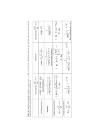
Stress and heat flux in the kinetic theory
In terms of the distribution function the densities of mass, momentum, and energy
can obviously be written as

37
That cumbersome word – even for German ears – describes a formula for the number of
collisions which lead to a particular scattering angle by the binary interaction of atoms.
The expression is not due to Maxwell, of course, nor to Boltzmann. As far as I can find
out it was first used by P. and T. Ehrenfest in “Conceptual Foundations of the Statistical
Approach in Mechanics.” Reprinted: Cornell University Press, Ithaca (1959).
The word seems to be untranslatable, and so it has been joined to the small lexicon of
German words in the English language like Kindergarten, Zeitgeist, Realpolitik and,
indeed, Ansatz.
Ludwig Eduard Boltzmann (1844–1906) 97

2
1
2
2
d, d, d
.
µ
u
2
ȡ µf c ȡ µc f c ȡ cfc
ii


ÔÔ Ô
X
X
u is the specific internal energy formed with C
i
= c
i
–
X
i
cfCuȡ
µ
d
2
2
³

.
With
6W
M
P
2
3
– appropriate for a monatomic ideal gas – we obtain
38
³
³

cf
cfC
kT
µ
d
d
2
2
2
3
so that T is the mean kinetic energy of the atoms. This may be considered as the
kinetic definition of temperature, or the kinetic temperature.
If
2
2
,,
E
K
E
P
PP\
is introduced into the equations of transfer, one obtains the
conservation laws of mass, momentum and energy
.0
d
2
2
d)
2
2

1
(
)
2
2
1
(
0
)d(
0

w
³

³
w

w
w

w
³
w

w
w

w
w


w
w
¸
¹
·
¨
©
§
i
x
cf
i
CC
µ
i
cf
i
C
j
Cµ
i
uȡ
t
uȡ
i
x
cf
i
C
j

Cµ
ij
ȡ
t
j
ȡ
i
x
i
ȡ
t
ȡ
Comparison with the corresponding macroscopic laws, cf. Chap. 3, identifies stress
and heat flux of a gas as
³

³

cf
i
CC
i
qcf
i
C
j
Cµ
ij
t
µ

d
2
2
andd
.
Thus the stress is properly called a momentum flux.
Insert. 4.4
For special choices of ȥ, viz. ȥ = µ, ȥ = µc
i
, ȥ =
1
/
2
µc
2
, one obtains the
conservation laws of mass, momentum and energy from the generic
equation, cf. Insert 4.4. In those cases both source terms vanish. For any
other choice of ȥ the collision term is not generally equal to zero.
However, there is an important choice of ȥ for which a conclusion can be
drawn, although the source does not vanish. That is the case when the
production has a sign. A sharp look at the source, – in the suggestive form
in which I have written it – will perhaps allow the attentive reader to
identify that particular ȥ all by himself. Certainly this was no difficulty for

38
The additive energy constant is routinely ignored in the kinetic theory.
98 4 Entropie as S = k ln W

39

All this is terribly anachronistic but it belongs here. Grad proposed the moment
approximation of the distribution function in 1949! H. Grad: “On the kinetic theory of
rarefied gases.” Communications of Pure and Applied Mathematics 2 (1949).
Boltzmann. He chose ȥ = –k ln
b
f
, where k and b are positive constants to
be determined. With that choice we have
collision source =
1
11 1
1
'
ln ( ' ) sin d d d d
4
kff
ff ff g
ff
σ θθϕ



Ô
cc
and that is obviously non-negative, since
1
1
'
ln
f

f
f
f

and )(
11
fff'f 
c
always have the same sign. In equilibrium, where f is given by the
Maxwellian distribution, both expressions vanish so that there is no source.
Both properties suggest that
³
 xcddln
b
f
f
M5
is a candidate for being considered as the entropy of the kinetic theory of
gases. If k is the Boltzmann constant, S is the entropy. Indeed, if we insert
the Maxwellian – the equilibrium distribution – we obtain
5
( , ) ( , ) ln ln
2
equ equ R R
RR
kTk p
STp STp m
Tp
µµ
ÈØ

 
ÉÙ
ÊÚ
which agrees with the entropy of a monatomic gas calculated by Clausius,
see Chap. 3.
Entropy flux
The interpretation of the quantity ln d
f
kf c
b

Ô
as entropy density is not complete
unless we relate its rate of change, or its flux, to heat or heating, so as to recognize
the status of Clausius’s 2nd law
T
Q
t
S

t
d
d
within the kinetic theory. Let us consider
that:
If indeed ln d d
f
kf cx
b
Ô

 is the entropy, the non-convective entropy flux should
be given by
ln d .
f
kC
f
c
ii
b
Φ 
Ô
We calculate that expression from the Grad 13-moment approximation
39
Ludwig Eduard Boltzmann (1844–1906) 99
2
2
11 1 11
11
25
()
Gequ ijij ii
ij
kk k
k
ff t CC qC C
ȡ TT T
ȡ T
µµ µ
µ
δ

ÈØ
ÉÙ
ÈØ ÈØ
ÉÙ
  
ÉÙ ÉÙ
ÉÙ
ÊÚ ÊÚ
ÉÙ
ÊÚ

,
which is the most popular – and most rational – approximate near-equilibrium
distribution function available. Insertion provides, if second order terms in ij are
ignored


2
and
22 2
5
3
4
5
tt tq
qq q
j
ij ij ij
ii i
ss

equ
i
kk
T
k
TT
µµ
T
µ
ȡȡ
ȡȡ
ȡ
Φ    .
Thus s contains non-equilibrium terms and
T
q
ĭ
i
i

– the Duhem expression for the
entropy flux, cf. Chap. 3 – holds only, if non-linear terms are neglected.
Insert. 4.5
Thus Boltzmann had given a kinetic interpretation for the entropy, an
interpretation in terms of the distribution function f and its logarithm. That
interpretation, however, is in no way intuitively appealing or suggestive,
and as such it does not provide the insight into the strategy of nature which
I have promised; not yet anyway.
In order to find a plausible interpretation, the integral for S has to be
discretized and extrapolated in the manner described in Insert 4.6. It is the

very nature of extrapolations that there are elements of arbitrariness in
them; they are not just corollaries. In the present case – in the reformulation
of the integral for S – I have emphasized the speculative nature of the extra-
polating steps by introducing them with a bold-face if.
The discretization stipulates that the element dxdc of the (x,c)-space has
a finite number P
dxdc
(say) of occupiable points (x,c) – occupiable by
atoms – and that P
dxdc
is proportional to the volume dxdc of the element with
a quantity Y as the factor of proportionality. Thus
1
/
Y
is the volume of the
smallest element, i.e. a cell, which contains only one point. In this manner
the (x,c)-space is quantized and indeed, Boltzmann’s procedure in this
context foreshadows quantization, although at this stage it may be
considered merely as a calculational tool rather than a physical argument.
And it was so considered by Boltzmann when he says: … it seems needless
to emphasize that [for this calculation] we are not concerned with a real
physical problem. And further on: … this assumption is nothing more than
an auxiliary tool.
40

40
L. Boltzmann (1872) loc.cit.
ij
100 4 Entropie as S = k ln W

If the occupancy N
xc
of all points, or cells, in dxdc is equal, Boltzmann
obtained by a suitable choice of b viz. b = eY, cf. Insert 4.6
!
1
ln
xc
P
xc
N
kS
3

,
where P is the total number of cells – of occupiable points – in the (x,c)-
space.
This is still not an easily interpretable expression, but it is close to one.
Indeed, if we multiply the factor N! into the argument of the logarithm, we
may write
S = k ln W , where
!
!
xc
P
xc
N
N
W
3

.
And that expression is interpretable, because W – by the rules of
combinatorics – is the number of realizations, often called microstates, of
the distribution {N
xc
} of N atoms. [The combinatorial rule is relevant here,
if the interchange of two atoms at different points (x,c) leads to different
realizations.]

We shall see later, cf. Chaps. 6 and 7 that it was S.N. Bose who took the cells seriously,
and gave them a value and a physical interpretation.
Reformulation of
³
 xc ddln
b
f
fkS
Let there be P
dxdc
occupiable points in the element dxdc and let P
dxdc
xc
atoms, cf. figure, so that we have
N
xc
P
dxdc
= f dxdc. Then the contribution
of dxdc to S may be written as

b
YN
PkN
b
f
kf
xc
xc
lnddln
dd xc
xc  
.ln
dd
¦

xc
2
ZE
ZE
ZE
D
;0
0M
Fig. 4.4 An element of (x,c)-space
The sum is really a sum over P
dxdc
equal terms. b may be chosen arbitrarily and we
choose b = eY, where e is the Euler number so that
Let further each point in dxdc be occupied by the same number N of

= Y
dxdc.
Ludwig Eduard Boltzmann (1844–1906) 101
¦
 
xc
xc
dd
)ln(ddln
P
xc
xcxcxc
NNNk
b
f
kf


xcdd
!
1
ln
P
xc
xc
N
k
.
The last step makes use of the Stirling formula lna! = alna-a, which can be applied,

if a – here N
xc
– is much larger than 1. Therefore the total entropy reads


P
xc
xc
N
kS
!
1
ln
,
where P is the total number of occupiable points in the (x,c)-space.
Insert 4.6
A first extrapolation of the formula for S is that we may now drop the
requirement that the values N
xc
within the element dxdc are all equal. This
may be a constraint appropriate to the kinetic theory of gases, – where there
is only one value f(x,c,t) characterizing the gas in the element – but it has no
status in the new statistical interpretation of S. In particular, it is now
conceivable that all atoms may be found in the same cell, so that they all
have the same position and the same velocity; in that case the entropy is
obviously zero, since there is only one realization for that distribution.
With S = k ln W we have a beautifully simple and convincing possibility
of interpreting the entropy, or rather of understanding why it grows: The
idea is that each realization of the gas of N atoms is a priori considered to
occur equally frequently, or to be equally probable. That means that the

realization where all atoms sit in the same place and have the same velocity
is just as probable as the realization that has the first N
1
atoms sitting in one
place (x,c) and all the remaining N – N
1
atoms sitting in another place, etc.
In the former case W is equal to 1 and in the latter it equals

!!
!
11
NNN
N

. In the
course of the irregular thermal motion the realization is perpetually
changing, and it is then eminently reasonable that the gas – as time goes
on – moves to a distribution with more possible realizations and eventually
to the distribution with most realizations, i.e. with a maximum entropy. And
there it remains; we say that equilibrium is reached.
So this is what I have called the strategy of nature, discovered and
identified by Boltzmann. To be sure, it is not much of a strategy, because it
consists of letting things happen and of permitting blind chance to take its
course. However, S = klnW is easily the second most important formula of
physics, next to E = mc
2
– or at a par with it. It emphasizes the random
102 4 Entropie as S = k ln W
component inherent in thermodynamic processes and it implies – as we

shall see later – entropic forces of considerable strength, when we attempt
to thwart the random walk of the atoms that leads to more probable
distributions.
However, the formula S = klnW is not only interpretable, it can also be
extrapolated away from monatomic gases to any system of many identical
units, like the links in a polymer chain, or solute molecules in a solution, or
money in a population, or animals in a habitat. Therefore S = klnW with the
appropriate W has a universal significance which reaches far beyond its
origin in the kinetic theory of gases.
Actually S = klnW was nowhere quite written by Boltzmann in this form,
certainly not in his paper of 1872
41
. However, it is clear from an article of
1877
42
that the relation between S and W was clear to him. In the first
volume of Boltzmann’s book on the kinetic theory
43
he revisits the
argument of that report; it is there – on pp. 40 through 42 –, where he comes
closest to writing S = klnW. The formula is engraved on Boltzmann’s
tombstone, erected in the 1930’s after the full significance had been
recognized, cf. Fig. 4.5. From the quotation in the figure we see that
Boltzmann fully appreciated the nature of irreversibility as a trend to distri-
butions of greater probability.
Since a given system of bodies can never
by itself pass to an equally probable state,
but only to a more probable one, … it is
impossibletoconstructa perpetuum mobile
which periodically returns to the original

state.
44

41
L. Boltzmann: (1872) loc.cit.
42
L. Boltzmann: „Über die Beziehung zwischen dem zweiten Hauptsatze der mechanischen
Wärmetheorie und der Wahrscheinlichkeitsrechnung respektive den Sätzen über das
Wärmegleichgewicht“. [On the relation between the second law of the mechanical theory
of heat and probability calculus, or the theories on the equilibrium of heat.]
Sitzungsberichte der Wiener Akademie, Band 76, 11. Oktober 1877.
43
L. Boltzmann: “Vorlesungen über Gastheorie I und II“. [Lectures on gas theory] Verlag
Metzger und Wittig, Leipzig (1895) and (1898).
44
L. Boltzmann: „Der zweite Hauptsatz der mechanischen Wärmetheorie“. [The second law
of the mechanical theory of heat] Lecture given at a ceremony of the Kaiserliche
Akademie der Wissenschaften on May, 29th, 1886. See also: E. Broda: “Ludwig
Boltzmann. Populäre Schriften”. Verlag Vieweg Braunschweig (1979) p. 26.
Fig. 4.5. Boltzmann’s tombstone on Vienna s central cemetery
’
Reversibility and Recurrence 103
Boltzmann’s lecture on the second law
45
closes with the words: Among
what I said maybe much is untrue but I am convinced of everything. Lucky
Boltzmann who could say that! As it was, all four bold-faced ifs on the
forgoing pages – all seemingly essential to Boltzmann’s eventual inter-
pretation of entropy – are rejected with an emphatic not so! by modern
physics:

x Neither is N
xc
equal for all (x,c) in dxdc,
x nor is it true that all
N
xc
>> 1,
x nor does the interchange of identical atoms lead to a new realization,
x nor is the arbitrary addition of N! quite so innocuous as it might seem.
And yet, S = klnW, or the statistical probabilistic interpretation stands
more firmly than ever. The formula was so plausible that it had to be true,
irrespective of its theoretical foundation and, indeed, the formula survived –
albeit with a different W – although its foundation was later changed consi-
derably, see Chap. 6.
Reversibility and Recurrence
If Clausius met with disbelief, criticism and rejection after the formulation
of the second law, the extent of that adversity was as nothing compared
with what Boltzmann had to endure after he had found a positive entropy
source in the kinetic theory of gases. And it did not help that Boltzmann
himself at the beginning thought – and said – that his interpretation was
purely mechanical. That attitude represented a challenge for the
mechanicians who brought forth two quite reasonable objections
the reversibility objection and the recurrence objection.
The discussion of these objections turned out to be quite fruitful, although it
was carried out with some acrimony – particularly the discussion of the
recurrence objection. It was in those controversies that Boltzmann came to
hammer out the statistical interpretation of entropy, i.e. the realization that S
equals k · lnW, which we have anticipated above. That interpretation is
infinitely more fundamental than the formal inequality for the entropy in the
kinetic theory which gave rise to it.

The reversibility objection was raised by Loschmidt: If a system of atoms
ran its course to more probable distributions and was then stopped and all
its velocities were inverted, it should run backwards toward the less

45
L. Boltzmann: (1886) loc. cit. p. 46.
104 4 Entropie as S = k ln W
probable distributions. This had to be so, because the equations of
mechanics are invariant under a replacement of time t by –t. Therefore
Loschmidt thought that a motion of the system with decreasing entropy
should occur just as often as one with increasing entropy. In his reply
Boltzmann did not dispute, of course, the reversibility of the atomic
motions. He tried, however, to make the objection irrelevant in a
probabilistic sense by emphasizing the importance of initial conditions. Let
us consider this:
By the argument that we have used above, all realizations, or microstates
occur equally frequently, and therefore we expect to see the distribution
evolve in the direction in which it can be realized by more microstates, –
irrespective of initial conditions; initial conditions are never mentioned in
the context. This cannot be strictly so, however, because indeed
Loschmidt’s inverted initial conditions are among the possible ones, and
they lead to less probable distributions, i.e. those with less possible
realizations. So, Boltzmann
46
argues that, among all conceivable initial
conditions, there are only a few that lead to less probable distributions
among many that lead to more probable ones. Therefore, when an initial
condition is picked at random, we nearly always pick one that leads to
entropy growth and almost never one that lets the entropy decrease.
Therefore the increase of entropy should occur more often than a decrease.

Some of Boltzmann’s contemporaries were unconvinced; for them the
argument about initial conditions was begging the question, and they
thought that it merely rephrased the a priori assumption of equal probability
of all microstates. However, the reasoning seems to have convinced those
scientists who were prepared to be convinced. Gibbs was one of them. He
phrases the conclusion succinctly by saying that an entropy decrease seems
(!) not to be impossible but merely improbable, cf. Fig. 4.6.
Kelvin
47
had expressed the reversibility objection even before Loschmidt
and he tried to invalidate it himself. After all, it contradicted Kelvin’s own
conviction of the universal tendency of dissipation and energy degradation,
which he had detected in nature. He thinks that the inversion of velocities
can never be made exact and that therefore any prevention of degradation is
short-lived, – all the shorter, the more atoms are involved.

46
L. Boltzmann: „Über die Beziehung eines allgemeinen mechanischen Satzes zum zweiten
Hauptsatz der Wärmetheorie“. [On the relation of a general mechanical theorem and the
second law of thermodynamics] Sitzungsberichte der Akademie der Wissenschaften Wien
(II) 75 (1877).
47
W. Thomson: „The kinetic theory of energy dissipation“ Proceedings of the Royal Society
of Edinburgh 8 (1874) pp. 325–334.
Reversibility and Recurrence 105
… the impossibility of an uncompensated
decrease of entropy seems to be reduced to an
improbability.
48
One of the more distinguished person who remained unconvinced for a

long time was Planck. He must have felt that he was too distinguished to
enter the fray himself. Planck’s assistant, Ernst Friedrich Ferdinand
Zermelo (1871–1953), however, was eagerly snapping at Boltzmann’s
heels.
49
Neither Boltzmann nor the majority of physicists since his time
have appreciated Zermelo’s role much; most present-day physics students
think that he was ambitious and brash, – and not too intelligent; they are
usually taught to think that Zermelo’s objections are easily refuted. And yet,
Zermelo went on to become an eminent mathematician, one of the founders
of axiomatic set theory. Therefore we may rely on his capacity for logical
thought.
50
And it ought to be recognized that his criticism moved Boltzmann
toward a clearer formulation of the probabilistic nature of entropy and,
perhaps, even to a better understanding of his own theory.
Zermelo had a new argument, because Jules Henri Poincaré (1854–1912)
had proved
51
that a mechanical system of atoms, which interact with forces
that are functions of their positions, must return – or almost return – to its

48
J.W. Gibbs: “On the equilibrium of heterogeneous substances.” Transactions of the
Connecticut Academy 3 (1876) p. 229.
49
To those who know the chain of command in German universities – particularly in the
19th century – it is inconceivable that Zermelo entered into a major discussion with a
celebrity like Boltzmann without the approval and encouragement of his mentor Planck.
Actually Planck was notoriously slow to accept new ideas, including his own, cf. Chap. 7.

50
Later Zermelo even helped to make statistical mechanics known among physicists by
editing a German translation of Gibbs’s “Elementary principles of statistical mechanics”,
see below.
51
H. Poincaré: „Sur le problème des trois corps et les équations de dynamique’’ [On the
three-body problem and the dynamical equations] Acta mathematica 13 (1890) pp.1–270.
See also : H. Poincaré: “Le mécanisme et l’expérience’’ [Mechanics and experience]
Revue Métaphysique Morale 1 (1893) pp. 534–537.
Fig. 4.6. Josiah Willard Gibbs
106 4 Entropie as S = k ln W
initial position. Clearly therefore, the entropy which, after all, is a function
of the atomic positions, cannot grow monotonically. This became known as
the recurrence objection. Actually, Zermelo thought that the fault lay in
mechanics, because he considered irreversibility to be too well established
to be doubted. But he could not bring himself to accept any of Boltzmann’s
probabilistic arguments.
52
In the controversy Boltzmann tried at first to get away with the
observation that it would take a long time for a recurrence to occur.
Zermelo agreed, but declared the fact irrelevant. The publicly conducted
discussion
53
,
,
54
,
,
55
,

,
56
then focussed on Boltzmann’s assertion that – at any one
time – there were more initial conditions leading to entropy growth than to
entropy decrease. Zermelo could not understand that assumption, and he
ridiculed it. In fact, however, something possibly profound came out of the
many words (!) – when he speculated that
… in the universe, which is nearly everywhere in an equilibrium, and
therefore dead, there must be relatively small regions of the dimensions of
our star space (call them worlds) … which, during the relatively short
periods of eons, deviate from equilibrium and among these [there must be]
equally many in which the probability of states increases and decreases. …
A creature that lives in such a period of time and in such a world will
denote the direction of time toward less probable states differently than the
reverse direction: The former as the past, the beginning, the latter as the
future, the end. With that convention the small regions, worlds, will
“initially” always find themselves in an improbable state.
Thus, over all worlds the number of initial conditions for growth and
decay of entropy may indeed be equal, although in some single world they
are not. It seems that Boltzmann believed that the universe as a whole is
essentially in equilibrium, but with occasional fluctuations of the size and

52
Ten years later Zermelo must have reconsidered this position. In 1906 he translated
Gibbs’s memoir on statistical mechanics into German, and surely he would not have
undertaken the task if he had still thought statistical or probabilistic arguments to be
unimportant. Zermelo’s translation helped to make Gibbs’s statistical mechanics known in
Europe.
53
E. Zermelo: “Über einen Satz der Dynamik und die mechanische Wärmelehre” [On a

theorem of dynamics and the mechanical theory of heat] Annalen der Physik 57 (1896)
pp. 485–494.
54
L. Boltzmann: “Entgegnung auf die wärmetheoretischen Betrachtungen des Hrn. E.
Zermelo” [Reply to the considerations of Mr. E. Zermelo on the theory of heat] Annalen
der Physik 57 (1896) pp. 773–784.
55
E. Zermelo: “Über mechanische Erklärungen irreversibler Vorgänge. Eine Antwort auf
Hrn. Boltzmanns “Entgegnung”. [“On mechanical explanations of irreversible processes.
A response to Mr. Boltzmann’s “reply”] Annalen der Physik 59 (1896), pp. 392–398.
56
L. Boltzmann: “Zu Hrn. Zermelos Abhandlung “Über die mechanische Erklärung
irreversibler Vorgänge” [On Mr. Zermelo’s treatise “On the mechanical explanation of
irreversible processes”] Annalen der Physik 59 (1896) pp. 793–801.
discussion. Boltzmann conceded the point – without ever admitting it in so
Maxwell Demon 107
duration of our own big-bang-world. A fluctuation will grow away from
equilibrium for a while and then relax back to equilibrium. In both cases the
subjective direction of time – as seen by a creature – is toward equilibrium,
irrespective of the fact that the growing fluctuation objectively moves away
from equilibrium. In order to make that mind-boggling idea more plausible,
Boltzmann
57
draws an analogy to the notions of up and down on the earth:
Men in Europe and its antipodes both think that they stand upright, while
objectively one of them is upside down. Applied to time, however, the idea
does not seem to have gained recognition in present-day physics; it is
ignored – at least outside science fiction. Maybe rightly so (?).
Boltzmann tries to anticipate criticism of his daring concept of time and
time reversal by saying:

Surely nobody will consider a speculation of that sort as an important
discovery or – as the old philosophers did – as the highest aim of science.
It is, however, the question whether it is justified to scorn it as something
entirely futile.
Actually we may suspect that Boltzmann was not entirely sincere when
he made that disclaimer. Indeed, in the years to come he is on record for
repeating his cosmological model several times. After having invented it in
the discussion with Zermelo he repeats it, and expands on it in his book on
the kinetic theory, and again in his general lecture at the World Fair in
St. Louis
58
.
All in all, the discussion between Boltzmann and Zermelo – despite
considerable acrimony – was conducted on a high level of sophistication
which definitely sets it off from the more pedestrian attempts of Maxwell
and Kelvin to come to grips with randomness and probability. Those
attempts involved the Maxwell demon.
Maxwell Demon
Maxwell invented the demon
59
in the effort to reconcile the irreversibility in
the trend toward a uniform temperature with the kinetic theory: … a
creature with such refined capabilities that it can follow the path of each
atom. It guards a slide valve in a small passage between two parts of a gas
with – initially – equal temperatures. The demon opens and closes the valve
so that it allows fast atoms from one side to pass, and slow atoms to pass

57
L. Boltzmann: (1898) loc. cit. p.129.
58

L. Boltzmann: “Über die statistische Mechanik” [On statistical mechanics] Lecture given
at a scientific meeting in connection with the World Fair in St. Louis (1904). See also:
E. Broda (1979) loc.cit. pp. 206–224.
59
According to G. Peruzzi (2000) loc.cit. p. 93 f. the demon was first conceived in a letter
by Tait to Maxwell in (1867). It appeared in print in Maxwell’s “Theory of Heat”
Longmans, Green & Co. London (1871).
108 4 Entropie as S = k ln W
from the other side. In this manner it creates a temperature difference
without work because, indeed, the valve has very little mass.
The Maxwell demon was – and is – much discussed, primarily, I suspect,
because it can happily be talked about by people who do not possess the
slightest knowledge of mathematics. In the works of Kelvin
60
the notion
reached absurd proportions: He invented … an army of intelligent Maxwell
demons which is stationed at the interface between a cold and a hot gas and
… equipped with clubs, molecular cricket bats, as it were. … Its mass is
several times as big as the molecules … and the demons must not leave
their assigned places except when necessary to execute their orders.
Enough of that! Brush
61
recommends an article by Klein
62
for the readers
who want to familiarize themselves with the voluminous secondary
literature on Maxwell’s demon. But we shall leave the subject as quickly as
possible. It has a touch of banality. We might just as well go into some
belly-aching over a demon that could improve our chances in a dice game.
Boltzmann and Philosophy

There is a persistent tale that Boltzmann committed suicide in a depressed
mood, created by discouragement and lack of recognition of his work. This
cannot be true. To be sure, eminent people do not take kindly to criticism,
and they become addicted to praise and may need it every hour of every
day; but Boltzmann did get that kind of attention: He was a celebrity with
an exceptional salary for the time and full recognition by all the people who
counted. Even the Zermelo controversy seems to have rankled in his mind
only slightly: In his essay “The Journey of a German Professor to Eldorado”
Boltzmann reports good-humouredly that Felix Klein tried to push him into
writing a review article on statistical mechanics by threatening to ask
Zermelo to do it, if Boltzmann continued to delay.
So, no! The neurasthenic condition which darkened Boltzmann’s life,
seems more like the depressing mood that afflicts a certain percentage of the
human population normally and which is nowadays treated effectively with
certain psycho-pharmaca, vulgarly known as happiness pills.
It is true though that Boltzmann did not reign supreme in the scientific
circles in Vienna; there was also Ernst Mach (1838–1916), a physicist of
some note in gas dynamics. Mach was a thorn in Boltzmann’s flesh,
because he insisted that physics should be restricted to what we can see,
hear, feel, and smell, or taste, and that excluded atoms. As late as 1897

60
W. Thomson: (1874) loc.cit.
61
S.G. Brush: (1976) loc.cit. p. 597.
62
M.J. Klein: American Science 58 (1970).
Boltzmann and Philosophy 109
63
and it is therefore clear that he

had no appreciation for the kinetic theory of gases. Mach also taught
philosophy and his classes were full of students eager to imbibe his tasty
intellectual philosophical concoction. Boltzmann taught hard science and
insisted that his students master a good deal of mathematics; consequently
there were few students. That situation irritated Boltzmann, and he decided
to teach philosophy himself.
He brought to the task a healthy contempt of philosophers. After Mach
had retired, Boltzmann taught Naturphilosophie in Vienna. And in his
inaugural lecture
64
he gave an account of the failure of his efforts to learn
something about philosophy:
So as to go to the deepest depths I picked up Hegel; but what an unclear,
senseless torrent of words I was to find there! My bad luck conducted me
from Hegel to Schopenhauer … and even in Kant there were many things
that I could grasp so little that, judging by the sharpness of his mind in
other respects, I almost suspected that he was pulling the reader’s leg, or
even deceiving him.
For a lecture to the philosophical society of Vienna he proposed the title:
Proof that Schopenhauer is a stupid, ignorant philosophaster, scribbling
nonsense and dispensing hollow verbiage that fundamentally and forever
rots people’s brains.
When the organizers objected, he pointed out – to no avail – that he was
merely quoting Schopenhauer, who had written these exact same words
about Hegel. Boltzmann had to change the title to a tame one: On a Thesis
of Schopenhauer,
65
but he got his own back by explaining the controversy in
detail to the audience: Apparently Schopenhauer wrote that sentence about
Hegel in a fit of pique, when Hegel had failed to support him for an

appointment to an academic position. In contrast to that Boltzmann’s
intended title had been chosen out of an objective evaluation of
Schopenhauer’s work, – or so he says.
It is thus clear that Boltzmann was not an optimal choice for a teacher of
conventional philosophy. His disdain for philosophy, that doctrine of clap-
trap and idle whim was expressed frequently, with or without provocation.
It is a good thing, perhaps, that Boltzmann did not also apply himself to the

63
I recommend an excellent account of Boltzmann’s professional work and psyche by D.
Lindley: “Boltzmann’s atom.” The Free Press, New York, London (2001). Lindley starts
his Introduction with the apodictic quotation from Mach: “I don´t believe that atoms
exist.”
64
L. Boltzmann: “Eine Antrittsvorlesung zur Naturphilosophie” [Inaugural lecture on natural
philosophy] Reprinted in the journal “Zeit” December 11, 1903 See also: E. Broda: loc.cit.
65
L. Boltzmann: “Über eine These von Schopenhauer” Lecture to the Philosophical Society
of Vienna, given on January 21, 1905. See also: E. Broda: loc.cit.
Mach maintained that atoms did not exist,
110 4 Entropie as S = k ln W
teaching of theology. Because indeed, his ideas in that field are again quite
unconventional as the following paragraph shows.
66
… only a madman denies the existence of God. However, it is true that all
our mental images of God are only inadequate anthropomorphisms, so that
the God whom we imagine does not exist in the shape in which we
imagine him. Therefore, if someone says that he is convinced of God’s
existence and someone else says that he does not believe in God, maybe
both think exactly the same…

Boltzmann sincerely admired Darwin’s discoveries, however. Indeed, there
is not a single public lecture in which he did not advertise Darwin’s work.
That work represents the type of natural philosophy that appealed to
Boltzmann. And it is true that there is some congeniality between the two
scientists in their emphasis upon the underlying randomness of either
thermodynamic processes or biological evolution: The vast majority of all
mutations are detrimental to the progeny, just as the vast majority of
collisions in a gas lead to more disorder. In contrast to a gas, however, the
small minority of advantageous mutative events is assisted by natural
selection so that nature can create order in living organisms. Natural
selection in this view plays the role of the infamous Maxwell demon, see
above.
67
Despite his partisanship for Darwin’s ideas Boltzmann professes to see
nothing in his convictions that runs counter to religion.
68
In the last ten years of his life Boltzmann did not really do any original
research, nor did he follow the research of others. Planck’s radiation theory
of 1900, and Einstein’s works on photons, on E = mc
2
, and on the Brownian
movement – all in 1905 – passed by him. In the end his neurasthenia
caught up with him in a summer vacation. He sent his family to the beach
and hanged himself in the pension on the crossbar of a window.

66
L. Boltzmann: “Über die Frage nach der objektiven Existenz der Vorgänge in der
unbelebten Natur” [On the question of the objective existence of events in the inanimate
nature] Sitzungsberichte der kaiserlichen Akademie der Wissenschaften in Wien.
Mathematisch-naturwissenschaftliche Klasse; Bd. CVI. Abt. II (1897) p. 83 ff.

67
Boltzmann does not seem to have argued like that. I read about this idea in one of
Asimov’s scientific essays. I. Asimov: “The modern demonology” in “Asimov on
Physics.” Avon Publishers of Bard, New York (1979).
68
Some church leaders see this differently. So also Pope Benedikt XVI. Says he in his
inaugural speech on April 24th, 2005: each being is a thought of God and not the
product of a blind evolutionary process. The catholic church does not like random
evolution, nor does George W. Bush, 43rd president of the United States of America, who
advocates that intelligent design be taught in the schools of his country.
Kinetic Theory of Rubber 111
Kinetic Theory of Rubber
We have already remarked that the formula S = klnW can be extrapolated
away from monatomic gases, where it was discovered. One such extra-
polation – an important one, and a particularly plausible one – occurred in
the 1930’s when chemists started to understand polymers and to use their
understanding to develop a thermal equation of state for rubber. The kinetic
theory of rubber is a masterpiece of thermodynamics and statistical
thermodynamics, and it laid the foundation for an important modern branch
of physics and technology: Polymer science.
At the base of the theory is the Gibbs equation, see Chap. 3. In the above
form the term –pdV represents the work done on the gas. That term must be
replaced by PdL for a rubber bar of length L under the uni-axial load P,
which depends on L and T, cf. Fig 4.7. Therefore the appropriate form of
the Gibbs equation for a bar reads
TdS = dU – PdL .
The Gibbs equation obviously implies
L
S
T

L
U
P
w
w

w
w

,
so that we may say that the load has an energetic and entropic part.
The integrability condition implied by the Gibbs equation reads
T
P
TP
L
U
w
w

w
w
and hence follows
T
P
L
S
w
w

w
w
.
Fig. 4.7. A rubber bar in the un-stretched and stretched configurations
112 4 Entropie as S = k ln W
Therefore the entropic part of the load may be identified as the slope of
the tangent of the easily measured (P,T)-curve of the bar for a fixed length
L. The energetic part is determined from the ordinate intercept of that
tangent, cf. Fig. 4.8.
Tangent identifies entropic and energetic parts of force
When the (P,T)-curve is measured for rubber it turns out to be a straight
line through the origin of the (P,T)-diagram. Therefore in rubber
L
S
w
w
is inde-
pendent of T, and U does not depend on L. We obtain
L
S
TP
w
w

(for rubber) ,
a relation that is sometimes expressed by saying that rubber elasticity is
entropic, or that the elastic force of rubber is entropy induced; energy plays
no role in rubber elasticity.
This was first noticed by Kurt H. Meyer and Cesare Ferri
69

and they
describe their discovery by saying: L´origine de la contraction [du
caoutchouc] se trouve dans l´orientation par la traction des chaînes
polypréniques. A cette orientation s´opposent les mouvements thermiques
qui provoquent finalement le retour des chaînes orientées à des positions
désordinées (variation de l´entropie).
70

69
K.H. Meyer & C. Ferri: “Sur l´élasticité du caoutchouc”. Helvetica Chimica Acta 29,
p. 570 (1935).
70
The cause for the contraction of rubber lies in the orientation imparted to the polymer
chains by the traction. The orientation is opposed by the thermal motion which eventually
causes the return of the oriented chains to disordered positions (change of entropy).
Left: (load, temperature)-curve for a generic material Right: ditto for rubber. Fig. 4.8.
Kinetic Theory of Rubber 113
It is clear then that we need S as a function of L, if we wish to calculate
the thermal equation of state P(T,L) of rubber. We know that S=klnW holds
and for the calculation of W we need a model for the chaînes desordineés,
the unordered polymer chains. Werner Kuhn (1899–1963)
72
has provided
such a model by imagining the rubber molecules as chains of N
independently oriented links of length b with an end-to-end distance r.
where N
±
links point to the right or left. Obviously for that simplified
model – which we use here – we must have
The pair of numbers

`^

NN ,

is called the distribution of links, and the
number of possible realizations of this distribution is

71
I. Müller, W. Weiss: “Entropy and energy – a universal competition” Springer,
Heidelberg (2005). In Chap. 5 of that book the analogy between thermodynamic properties
of rubber and gases is highlighted by a juxtaposition.
72
W. Kuhn: “Über die Gestalt fadenförmiger Moleküle in Lösungen” [On the shape of
filiform molecules in solution] Kolloidzeitschrift 68, p. 2 (1934).
Fig. 4.9. Model for rubber molecule and its one-dimensional caricature
Apart from rubber, and some synthetic polymers, entropic elasticity occurs only
in gases. Indeed, different as gases and rubber may be in appearance,
thermodynamically those materials are virtually identical. A joker with an original
turn of mind has once commented on this similarity by saying that rubbers are the
ideal gases among the solids.
71
Fig. 4.9 shows such a molecule and also its one-dimensional caricature,
TD0D0
0D
T0
0
000

r



r

1
(
2
hence
.
(
°
°
r
°
°
114 4 Entropie as S = k ln W
!!
!!
1!1!
22
NN
W
NN
NrNr
Nb Nb



ËÛËÛ
ÈØÈØ
ÉÙÉÙ

ÌÜÌÜ
ÊÚÊÚ
ÍÝÍÝ
.
Thus W and S
mol
= klnW, the entropy of a molecule, are functions of the
end-to-end distance r. That function may be simplified by use of the Stirling
formula and by an expansion of the logarithm, viz.
lna! = alna-a and ln
2
1
1
2
rrr
Nb Nb Nb
ÈØ ÈØ

ÉÙ ÉÙ
ÊÚ ÊÚ
.
The former is true for large values of a, and we apply it to N as well as to
.
r
N The approximation of the logarithm is good for 1
Nb
r
, i.e. for a
strong degree of folding of the molecular chain. We obtain
2

1
ln 2
2
mol
r
SNk
Nb
ÈØ
ÈØ

ÉÙ
ÉÙ
ÊÚ
ÊÚ
,
so that the entropy of the molecule is maximal when its end-to-end distance
is small.
notion of entropy and its growth property, more – perhaps – than the
understanding of gases. Let us consider:
any other one during the course of the thermal motion. This means in
particular that the fully stretched-out microstate shown in Fig. 4.10 occurs
just as frequently as the partially folded microstate of the figure with the
end-to-end distance r < Nb. This means also, however, that a folded
distribution
`^

NN ,
with r < Nb occurs more frequently than the fully
stretched distribution
`^

0,N
, because the former can be realized by more
microstates, while the latter has only one realization.
°
°
°
°
r
r=Nb
Fig. 4.10. Fully stretched and folded realizations of the chain molecule
The basic a priori axiom is: Equal probability of all realizations or
The understanding of the rubber molecule does a lot for grasping the
microstates.Thus each and every microstate occurs just as frequently as
Kinetic Theory of Rubber 115
Therefore, if the chain molecule starts out straight – with W = 1, i.e.
S
mol
= 0 – the thermal motion will very quickly mess it up, and kick the
molecule into a distribution with many microstates and eventually – with
overwhelming probability – into the distribution with most microstates,
which we call equilibrium. In equilibrium we therefore have N
+
= N
-
=
1
/
2
so
that r is zero. During that process the entropy S

mol
grows from zero to
!!
!
22
ln
NN
N
k . Thus the entropy growth is the result of a random walk of the
chain between its microstates.
Of course, we can prevent this growth. If we wish to maintain the straight
microstate, – or any r in the interval 0 < r < Nb – we need only give the
molecule a tug at the ends each time when the thermal motion kicks it. And,
if the thermal motion kicks the molecule 10
12
times per second – a reason-
able number – we may apply a constant force at the ends. That is the nature
of entropic forces and of entropic elasticity. And that is the nature of the
force needed to keep a rubber molecule extended. If r << Nb, the entropy is
linear in r
2
, see above, and the force is proportional to r with the factor of
proportionality linear in T, the temperature: The more vigorous the thermal
motion is, the bigger is the entropic force. Mechanicians like to speak of the
entropic spring; its hallmark is an elastic modulus proportional to T.
It is often said that the value of the entropy of a distribution is a measure
for the disorder in the arrangement of its particles. This interpretation is
most easily understood for the rubber molecule. Indeed, the stretched out,
orderly distribution of Fig. 4.10 has zero entropy, because it can only be
realized in one single manner. The disordered, folded distribution has

positive entropy. And the most disorderly distribution with very many
possible realizations has the maximum value of entropy. Therefore the
growth of entropy toward equilibrium involves a growth of disorder.
A rubber bar consists of a network of rubber molecules all with different
length vectors (ș
1
,ș
2
,ș
3
) and different lengths
2
3
2
2
2
1
TTT r
, as shown in
Fig. 4.7. Thus the entropies in the un-stretched and stretched states are
given, respectively, by
Having said this I like to stress that order and disorder are not well-defined
physical concepts. To be sure, in the present context the notions jibe with our
intuition, but they do not always do that. Thus a cubic lattice in an alloy – judged
well-ordered on intuitive grounds – has a higher entropy than the more disorderly
monoclinic lattice. For that reason the cubic phase is often the high-temperature
phase, because for higher temperature the entropy becomes more important in the
free energy, cf. Chap. 5. This apparent violation of the equivalence of entropy and
disorder can be explained, but the explanation does not employ the notion of
crystallographic order or disorder.

116 4 Entropie as S = k ln W
³
TTTTTT
32132100
),,( dddzSS
mol
and
³
TTTTTT
321321
),,( dddzSS
mol
,
where z
0
(ș
1
,ș
2
,ș
3
)dș
1
dș
2
dș
3
and z(ș
1
,ș

2
,ș
3
)dș
1
dș
2
dș
3
are the numbers of
distance vectors in the interval dș
1
dș
2
dș
3
at ș
1
,ș
2
,ș
3
.
The determination of the functions z
0
(ș
1
,ș
2
,ș

3
) and z(ș
1
,ș
2
,ș
3
) is again due
to Kuhn in 1936.
73
For the argument he ingeniously employed the inversion
of S
mol
= klnW : He assumed the number z
0
(ș
1
,ș
2
,ș
3
)dș
1
dș
2
dș
3
to be
proportional to the number W = exp{S
mol

/k} of realizations of chains with
2
3
2
2
2
1
TTT r
and obtained
222
123
0123
32
2
(, , ) exp
2
2
n
z
Nb
Nb
θθθ
θθθ
π
ÎÞ

ÑÑ

Ïß
ÑÑ

Ðà
,
where n is the total number of chains. As for the number z(ș
1
,ș
2
,ș
3
)dș
1
dș
2
dș
3
Kuhn assumed that
123 0 1 2 3
1
(, , ) , ,zzθ θ θ θ λθ λθ
λ
ÈØ

ÉÙ
ÊÚ
holds, so that the components of the length vectors are deformed exactly as
the edges of the (incompressible) rubber bar, whose deformation in the
direction of the force is given by L = ȜL
0.
Thus Kuhn obtained
2
0

123
22
SS nkλ
λ
ÈØ
 
ÉÙ
ÊÚ
and
2
0
1nkT
P
L
λ
λ
ÈØ

ÉÙ
ÊÚ
.
The latter formula represents the thermal equation of state of a rubber bar
which gives the load as a function of the temperature Tand the stretch
Ȝ =
L
/
Lo
. The (P,Ȝ)-relation is obviously non-linear.
74
and the field of

non-linear elasticity. Its derivation provides a deep insight into the

73
W. Kuhn: “Beziehungen zwischen Molekülgröße, statistischer Molekülgestalt und
elastischen Eigenschaften hochpolymerer Stoffe” [Relations between molecular size,
p. 258 (1936).
74
Modern representations of the field may be found in the monograph by P.J. Flory:
“Principles of Polymer Chemistry.” Cornell University Press, Ithaca (1953). The book has
gone through many editions and re-printings in later years.
This formula marks the beginning of polymer science
statistical molecular shape and elastic properties of high polymers] Kolloidzeitschrift 76,