100 STATISTICAL TESTS phần 8 potx

GOKA: “CHAP05D” — 2006/6/10 — 17:23 — PAGE 167 — #31
THE TESTS 167
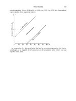
rejection number. If θ
0
= 0.04 and θ
1
= 0.08, α = 0.15, β = 0.25, then the graphical
representation of the sequential plan is:
As soon as (m, S
m
) lies on or below the line for a
m
or on or above the line for r
m
,
sampling is to be stopped; the new process is to be considered in the former case and
rejected in the latter.
GOKA: “CHAP05D” — 2006/6/10 — 17:23 — PAGE 168 — #32
168 100 STATISTICAL TESTS
Test 91 Sequential probability ratio test
Object
A sequential test for the ratio between the mean and the standard deviation of a normal
population where both are unknown.
Limitations
This test is applicable if the observations are normally distributed with unknown mean
and variance.
Method
Let X ∼ N(µ, σ
2
), where both µ and σ
2

are unknown. We want to find a sequential
test for testing H
0
: µ/σ = r
0
against H
1
: µ/σ = r
1
. The sequential probability ratio
test procedure is as follows.
1. Continue sampling if b
n
< t
n
< a
n
, where
t
n
=
n

i=1
X
i





n

i=1
X
2
i
=
n

i=1
y
i




n

i=1
y
2
i
where y
i
= X
i
/|X
i
|, i = 1, 2, , n,
a

n
= log
1 − β
α
and b
n
= log
β
1 − α
.
2. Fail to reject H
0
if t
n
 b
n
and reject H
0
if t
n
 a
n
.
Example
A useful measure is the ratio of mean divided by standard deviation since it is inde-
pendent of measured units. Here we set up a sequential test for the ratio equal to 0.2
versus the alternative that it is equal to 0.4. The rule is that if the test statistic is less
than log(7/15) do not reject the null hypothesis and if the test statistic is greater than
log(13/5) then reject the null hypothesis; otherwise continue to sample.
Numerical calculation

Consider a sample from N(µ, σ
2
) where µ and σ are both unknown. Then we want a
sequential test for testing H
0
: µ/σ = 0.2 against H
1
: µ/σ = 0.4.
Let α = 0.25, β = 0.35, a
n
= log(0.65/0.25), b
n
= log(0.35/0.75).
If log 7/15 < t
n
< log 13/5 then continue sampling.
If t
n
 log 7/15 do not reject H
0
, and if t
n
 log 13/5 reject H
0
.
GOKA: “CHAP05D” — 2006/6/10 — 17:23 — PAGE 169 — #33
THE TESTS 169
Test 92 Durbin–Watson test
Object
To test whether the error terms in a regression model are autocorrelated.

Limitations
This test is applicable if the autocorrelation parameter and error terms are independently
normally distributed with mean zero and variance s
2
.
Method
This test is based on the first-order autoregressive error model ε
t
= ϕε
t−1
+ u
t
where
ϕ is the autocorrelation parameter and the u
t
, are independently normally distributed
with zero mean and variance σ
2
. When one is concerned with positive autocorrelation
the alternatives are given as follows:
H
0
: ϕ  0 H
1
: ϕ>0.
Here H
0
implies that error terms are uncorrelated or negatively correlated, while H
1
implies that they are positively autocorrelated. This test is based on the difference

between adjacent residuals ε
t
− ε
t−1
and is given by
d =
n

t=2
(e
t
− e
t−1
)
2
n

t=1
e
2
t
where e
t
is the regression residual for period t, and n is the number of time periods
used in fitting the regression model.
When the error terms are positively autocorrelated the adjacent residuals will tend to
be of similar magnitude and the numerator of the test statistic d will be small. If the error
terms are either not correlated or negatively correlated e
t
and e

t−1
will tend to differ
and the numerator of the test statistic will be larger. The exact action limit for this test
is difficult to calculate and the test is used with lower bound d
L
and the upper bound
d
U
. When the statistic d is less than the lower bound d
L
, we conclude that positive
autocorrelation is present. Similarly, when the test statistic exceeds the upper bound
d
U
, we conclude that positive autocorrelation is not present. When d
L
< d < d
U
, the
test is inconclusive.
Example
Data on the sales (£m) of a large company (Y) compared with its sector total (X) have
been collected over a five-year period. In order to test the significance of the regression
of Y on X, and to obtain confidence intervals on predictions, it is necessary to perform a
test of serial correlation on the error term or residuals. The Durbin–Watson test statistic
GOKA: “CHAP05D” — 2006/6/10 — 17:23 — PAGE 170 — #34
170 100 STATISTICAL TESTS
(d) is equal to 0.4765 and is less than the lower d value (d
L
) of 1.20 [Table 33]. So the

residuals are positively autocorrelated. An appropriate adjustment to the error sum of
squares is necessary.
Numerical calculation
n = 20, α = 0.05
Quarter-t Company sale Industry sales
Y
i
X
i
1 77.044 746.512
2 78.613 762.345
3 80.124 778.179
4––
–––
–––
–––
–––
20 102.481 1006.882
A computer run of a regression package provided us with the value of the test statistic
d = 0.4765: d
L
= 1.20 and d
U
= 1.41 from Table 33. Since d = 0.4765 < 1.20, the
error terms are positively autocorrelated.
GOKA: “CHAP05D” — 2006/6/10 — 17:23 — PAGE 171 — #35
THE TESTS 171
Test 93 Duckworth’s test for comparing the medians
of two populations
Object

A quick and easy test for comparing the medians of two populations which could be
used for a wide range of m and n observations.
Limitations
This is not a powerful test but it is easy to use and the table values can be easily obtained.
It works only on the largest and the smallest values of the observations from different
populations.
Method
Consider the smallest observation from the X population and the largest from the Y
population. Then the test statistic, D, is the sum of the overlaps, the number of X
observations that are smaller than the smallest Y , plus the number of Y observations
that are larger than the largest X. If either 3 +4n/3
 m  2n or vice versa we subtract
1 from D. Under these circumstances, the table of critical values consists of the three
numbers; 7, 10 and 13. If D
 7 we reject the hypothesis of equal medians at α = 0.05.
Example
Two groups of workers are compared in terms of their daily rates of pay. Are they
significantly different? We use Duckworth’s test since the median is an appropriate
measure of central tendency for an income variable. The test statistic is 5 which is less
than 7 and so not significant. We have no reason to assume any difference in rates of
pay between the two groups.
Numerical calculation
m = n = 12
123456789101112
66.3 68.3 68.5 69.2 70.0 70.1 70.4 70.9 71.1 71.2 72.1 72.1
XXXYYXXYXXYY
13 14 15 16 17 18 19 20 21 22 23 24
72.1 72.7 72.8 73.3 73.6 74.1 74.2 74.6 74.7 74.8 75.5 75.8
XXYYXXYYYXYY
We note that there are three X observations below all the Y observations and two Y s

above all the Xs. The total is D = 5, which is less than 7 and so not significant.
GOKA: “CHAP05D” — 2006/6/10 — 17:23 — PAGE 172 — #36
172 100 STATISTICAL TESTS
Test 94 χ
2
-test for a suitable probabilistic model
Object
Many experiments yield a set of data, say X
1
, X
2
, , X
n
, and the experimenter is often
interested in determining whether the data can be treated as the observed values of the
random sample X
1
, X
2
, , X
n
from a given distribution. That is, would this proposed
distribution be a reasonable probabilistic model for these sample items?
Limitations
This test is applicable if both distributions have the same interval classification and the
same number of elements. The observed data are observed by random sampling.
Method
Let X
1
denote the number of heads that occur when coins are tossed at random, under

the assumptions that the coins are independent and the probability of heads for each
coin has a binomial distribution. An experiment resulted in certain observed values at
Y
i
corresponding to 0, 1, 2, 3 and 4 heads.
Let A
1
={0}, A
2
={1}, A
3
={2}, A
4
={3}, A
5
={4} be the corresponding heads
and if π
i
= P(X ∈ A
i
) when X is B(4,
1
2
), then we have
π
1
= π
5
=


4
0

1
2

4
= 0.0625
π
2
= π
4
=

4
1

1
2

4
= 0.25
π
3
=

4
2

1

2

4
= 0.375.
If α = 0.05, then the null hypothesis
H
0
: p
1
= π
1
, p
2
= π
2
, p
3
= π
3
, p
4
= π
4
, p
5
= π
5
is rejected if the calculated value is greater than the tabulated value using

q

k−1
=
k

i=1
(y
i
− nπ
i
)
2
nπ
i

∼ χ
2
k−1
.
Example
We wish to test whether a binomial distribution is a good model for an application area.
A full group of prisoner trainees consists of up to five members. Each full group must
have two escorts if five members turn up for training. If up to three turn up for training
then only one escort is needed. Data is collected over 100 group turnouts. Is a binomial
GOKA: “CHAP05D” — 2006/6/10 — 17:23 — PAGE 173 — #37
THE TESTS 173
model a good fit? The calculated chi-squared statistic of 4.47 is less than the critical
value of 9.49 [Table 5] so a binomial model is an acceptable model for this data.
Numerical calculation
In this case y
1

= 7, y
2
= 18, y
3
= 40, y
4
= 31 and y
5
= 4. The computed value is
q
4
=
(7 − 6.25)
2
6.25
+
(18 − 25)
2
25
+
(40 −37.5)
2
37.5
+
(31 − 25)
2
25
+
(4 − 6.25)
2

6.25
= 4.47.
Critical value χ
2
4
(0.05) = 9.49 [Table 5].
Hence the hypothesis is not rejected. Thus the data support the hypothesis that B(4,
1
2
)
is a reasonable probabilistic model for X.
GOKA: “CHAP05D” — 2006/6/10 — 17:23 — PAGE 174 — #38
174 100 STATISTICAL TESTS
Test 95 V -test (modified Rayleigh)
Object
To test whether the observed angles have a tendency to cluster around a given angle
indicating a lack of randomness in the distribution.
Limitations
For grouped data the length of the mean vector must be adjusted, and for axial data all
angles must be doubled.
Method
Given a random sample of n angular values 
1
, 
2
, , 
n
and a given theoretical
direction determined by an angle θ
0

, then the test statistic for the test of randomness is:
V = (2n)
1
2
ϑ
where ϑ = r cos(
¯
 − θ
0
) and r is the length of the mean vector
r =
1
n
+



cos 
i

2
+


sin 
i

2

= (¯x

2
+¯y
2
)
1
2
¯
 =
⎧
⎪
⎪
⎨
⎪
⎪
⎩
arctan

¯y
¯x

if ¯x > 0
180
◦
+ arctan

¯y
¯x

if ¯x < 0.
If V is greater than or equal to the critical V (α), the null hypothesis, that the parent

population is uniformly distributed (randomness), is rejected.
Example
A radar screen produces a series of traces; angles from a centre are measured. Do these
cluster around a value of 265 degrees? The calculated V statistic is 3.884, which is
greater than the critical value of 2.302 [Table 34]. So the angles are not random and do
cluster.
Numerical calculation
n = 15

1
= 250
◦
, 
2
= 275
◦
, 
3
= 285
◦
, 
4
= 285
◦
, 
5
= 290
◦
, 
6

= 290
◦
,

7
= 295
◦
, 
8
= 300
◦
, 
9
= 305
◦
, 
10
= 310
◦
, 
11
= 315
◦
, 
12
= 320
◦
,

13

= 330
◦
, 
14
= 330
◦
, 
15
= 5
◦
, θ
0
= 265
◦
¯x =
1
n
(cos 
1
+···+cos 
15
) =
7.287
15
= 0.4858
GOKA: “CHAP05D” — 2006/6/10 — 17:23 — PAGE 175 — #39
THE TESTS 175
¯y =
1
n

(sin 
1
+···+sin 
15
) =
−11.367
15
=−0.7578
r = (¯x
2
+¯y
2
)
1
2
= (0.4858
2
+ 0.7578
2
)
1
2
= 0.9001
¯
 = arctan

−0.7578
0.4858

=−57.3

◦
, which is equivalent to 303
◦
.
ϑ = r cos(
¯
 − θ
0
) = 0.9001 × cos(303
◦
− 265
◦
) = 0.9001 × 0.7880 = 0.7093
V = (2 × 15)
1
2
× 0.7093 = 5.4772 ×0.7092 = 3.885
Critical value V
15; 0.01
= 2.302 [Table 34].
Hence reject the null hypothesis of randomness.
GOKA: “CHAP05D” — 2006/6/10 — 17:23 — PAGE 176 — #40
176 100 STATISTICAL TESTS
Test 96 Watson’s U
2
n
-test
Object
To test whether the given distribution fits a random sample of angular values.
Limitations

This test is suitable for both unimodal and the multimodal cases. The test is very
practical if a computer program is available. It can be used as a test for randomness.
Method
Given a random sample of n angular values 
1
, 
2
, , 
n
rearranged in ascending
order: 
1
 
2
 ··· 
n
. Suppose F() is the distribution function of the given
theoretical distribution and let
V
i
= F(
i
), i = 1, 2, , n
¯
V =
1
n

V
i

and C
i
= 2i − 1.
Then the test statistic is:
U
2
n
=
n

i=1
V
2
i
−
n

i=1

C
i
V
i
n

+ n

1
3
−


¯
V −
1
2

2

.
If the sample value of U
2
n
exceeds the critical value the null hypothesis is rejected.
Otherwise the fit is satisfactory.
Example
A particle atomizer produces traces on a filter paper, which is calibrated on an angular
scale. Are the particles equally spaced on an angular scale? The distribution is one
of equal angles and the calculated U squared statistic is 0.1361. This is smaller than
the critical value of 0.184 [Table 35] so the null hypothesis of no difference from the
theoretical distribution is accepted.
Numerical calculation
n = 13, F() = /360
◦
, 
1
= 20
◦
, 
2
= 135

◦
, 
3
= 145
◦
, 
4
= 165
◦
,

5
= 170
◦
, 
6
= 200
◦
, 
7
= 300
◦
, 
8
= 325
◦
, 
9
= 335
◦

, 
10
= 350
◦
,

11
= 350
◦
, 
12
= 350
◦
, 
13
= 355
◦
V
i
= 
i
/13, i = 1, ,13

V
i
= 8.8889,

V
2
i

= 7.2310,

C
i
V
i
/n = 10.9893,
¯
V = 0.68376
U
2
n
= 7.2310 − 10.9893 + 13

1
3
− (0.18376)
2

= 0.1361
Critical value U
2
13; 0.05
= 0.184 [Table 35].
Do not reject the null hypothesis. The sample comes from the given theoretical
distribution.
GOKA: “CHAP05D” — 2006/6/10 — 17:23 — PAGE 177 — #41
THE TESTS 177
Test 97 Watson’s U
2

-test
Object
To test whether two samples from circular observations differ significantly from each
other with regard to mean direction or angular variance.
Limitation
Both samples must come from a continuous distribution. In the case of grouping the
class interval should not exceed 5
◦
.
Method
Given two random samples of n and m circular observations 
1
, 
2
, , 
n
and

1
, 
2
, , 
m
, let n + m = N and d
1
, d
2
, , d
N
(k = 1, 2, , N) be the differ-

ences between the sample distribution function, and let
¯
d denote the mean of the N
differences. Then the test statistic is given by:
U
2
=
nm
N
2
⎡
⎣
N

k=1
d
2
k
−
1
N

N

k=1
d
k

2
⎤

⎦
.
If U
2
> U
2
(α), reject the null hypothesis.
Example
Two prototype machines produce two angular displacement scales. Are they essentially
the same with regard to mean direction and angular variance? The calculated U squared
statistic is 0.261. Since this is greater than the critical value of 0.185 [Table 36] the null
hypothesis of no difference is rejected. The two prototype machines differ.
Numerical calculation
n = 8, m = 10,
16

k=1
d
k
= 6.525,
16

k=1
d
2
k
= 3.422
U
2
=

80
18
2

3.422 −
6.525 × 6.525
18

= 0.261
Critical value U
2
8,10; 0.05
= 0.185 [Table 36].
The calculated value is greater than the critical value.
Reject the hypothesis. The two samples deviate significantly from each other.
GOKA: “CHAP05D” — 2006/6/10 — 17:23 — PAGE 178 — #42
178 100 STATISTICAL TESTS
Test 98 Watson–Williams test
Object
To test whether the mean angles of two independent circular observations differ
significantly from each other.
Limitations
Samples are drawn from a von Mises distribution and the concentration parameter
k (>2) must have the same value in each population.
Method
Given two independent random samples of n and m circular observations

1
, 
2

, , 
n
and 
1
, 
2
, , 
m
, for each sample, calculate the components of
the resultant vectors
C
1
=
n

i=1
cos 
i
S
1
=
n

i=1
sin 
i
C
2
=
m


i=1
cos 
i
S
2
=
m

i=1
sin 
i
with the resultant lengths
R
1
= (C
2
1
+ S
2
1
)
1
2
R
2
= (C
2
2
+ S

2
2
)
1
2
.
The directions of the resultant vectors are given by
¯
 and
¯
. For the combined sample,
the components of the resultant vector are
C = C
1
+ C
2
and S = S
1
+ S
2
.
Hence, the length of the resultant vector is
R = (C
2
+ S
2
)
1
2
.

To test the unknown mean angles of the population use the test statistic
F = g(N − 2)
R
1
+ R
2
− R
N − (R
1
+ R
2
)
where N = n +m and g = 1 − 3/8
ˆ
k, with k determined from
¯
R =
R
1
+ R
2
N
and Table 37. Reject the null hypothesis if the calculated value F is greater than the
critical value F
1, N−2
.
GOKA: “CHAP05D” — 2006/6/10 — 17:23 — PAGE 179 — #43
THE TESTS 179
Example
A trainee-building surveyor has calibrated two angular measuring devices. Do they

produce similar results? She takes ten measurements from each device and then uses
the Watson–Williams test to compare them. Her F test statistic is 8.43, which is greater
than the critical value of 8.29 [Table 3]. So the null hypothesis of no difference between
the samples is rejected suggesting that the two devices have been calibrated differently.
Numerical calculation
n = 10, m = 10, N = 20, ν
1
= 1, ν
2
= N − 2
C
1
= 9.833, C
2
= 9.849, C = 19.682
S
1
=−1.558, S
2
= 0.342, S =−1.216
R
1
= 9.956, R
2
= 9.854, R = 19.721
¯
R = 0.991 for
ˆ
k greater than 10, g = 1
ˆ

k = 50.241 [Table 37]
F =
18 × 0.089
0.190
= 8.432
Critical value F
1,18; 0.01
= 8.29 [Table 3].
Reject the null hypothesis.
Hence the mean directions differ significantly.
GOKA: “CHAP05D” — 2006/6/10 — 17:23 — PAGE 180 — #44
180 100 STATISTICAL TESTS
Test 99 Mardia–Watson–Wheeler test
Object
To test whether two independent random samples from circular observations differ
significantly from each other regarding mean angle, angular variance or both.
Limitation
There are no ties between the samples and the populations have a continuous circular
distribution.
Method
Consider two independent samples of n and m circular observations 
1
, 
2
, , 
n
and

1
, 

2
, , 
m
. We observe the order in which the random samples are arranged and
then alter the space between successive sample points in such a way that all these spaces
become the same size. Having spaced the sample points equally, the sample points are
then ranked. Let r
1
, r
2
, , r
n
be the ranks of the first sample and β
i
= r
i
δ(i = 1, , n)
be the angles, where δ and N = n +m are known as uniform scores. Then the resultant
vector of the first sample has components
C
1
=

cos β
i
S
1
=

sin β

i
and the length of the resultant vector is
R
1
= (C
2
+ S
2
)
1
2
.
The test statistic is given by
B = R
2
1
.
If B > B
α
, reject the null hypothesis. When N > 17, the quantity χ
2
= 2(N −1)R
2
1
/nm
has a χ
2
-distribution with 2 degrees of freedom if H
0
is true.

Example
A new improved boat navigation system is compared with the old one. Is the way they
work similar in terms of the observations taken? A sailor uses the Mardia–Watson–
Wheeler test and computes a B statistic of 3.618. This is smaller than the tabulated
value of 9.47 [Table 37] so he concludes that there is no difference between the two
systems.
Numerical calculation
n = 6, m = 4, N = 10, δ = 360
◦
/10 = 36
◦
, α = 0.05
Here m is the smaller sample size.
For the first sample:
r
1
= 1, r
2
= 2, r
3
= 3, r
4
= 4, r
5
= 8, r
6
= 9
GOKA: “CHAP05D” — 2006/6/10 — 17:23 — PAGE 181 — #45
THE TESTS 181
β

1
= 36
◦
, β
2
= 72
◦
, β
3
= 108
◦
, β
4
= 144
◦
, β
5
= 288
◦
, β
6
= 324
◦
C
1
= 1.118, S
1
= 1.539, R
1
= 1.902

B = 3.618
Critical value B
N, m; α
= B
10, 4; 0.05
= 9.47 [Table 38].
The calculated value B is less than the critical value B
α
.
Hence there are no significant differences between the samples. (The second sample
would lead to the same result.)
GOKA: “CHAP05D” — 2006/6/10 — 17:23 — PAGE 182 — #46
182 100 STATISTICAL TESTS
Test 100 Harrison–Kanji–Gadsden test (analysis of
variance for angular data)
Object
To test whether the treatment effects of the q independent random samples from von
Mises populations differ significantly from each other.
Limitations
1. Samples are drawn from a von Mises population.
2. The concentration parameter k has the same value for each sample.
3. k must be at least 2.
Method
Given a one-way classification situation with µ
0
, β
j
and e
ij
denoting the overall mean

direction, treatment effect and random error variation respectively, then

ij
= µ
0
+ β
j
+ e
ij
, i = 1, , p; j = 1, 2, , q
where each observation 
ij
is an independent observation from a von Mises distribution
with mean µ
0
+ β
j
and concentration parameter k.
For the one-way situation, the components of variation are similarly
k

N −
R
2
N

= k
⎡
⎣
q


j=1

R
2
·j
N
·j
−
R
2
N

⎤
⎦
+ k
⎡
⎣
N −
q

j=1

R
2
·j
N
·j

⎤

⎦
(Total variation) = (Between variation) + (Residual variation)
and the test statistic for a large value of k is given by
F

q−1,N−q
= β
⎡
⎢
⎢
⎢
⎢
⎢
⎢
⎣
(N − q)
⎛
⎝
q

j=1

R
2
·j
N
·j

−
R

2
N
⎞
⎠
(q − 1)
⎧
⎨
⎩
N −
q

j=1

R
2
·j
N
·j

⎫
⎬
⎭
⎤
⎥
⎥
⎥
⎥
⎥
⎥
⎦

where

p
i=1

q
j=1
cos(
ij
−ˆµ
0
) = R, and
¯

·j
are the jth mean angles with
corresponding resultant length r
·j
.
Let x
·i
and y
·j
be the rectangular components of r
·j
. Then:
r
··
=
⎡

⎢
⎣
⎛
⎝
1
q
q

j=1
r
·j
cos
¯

·j
⎞
⎠
2
+
⎛
⎝
1
q
q

j=1
r
·j
sin
¯


·j
⎞
⎠
2
⎤
⎥
⎦
1
2
GOKA: “CHAP05D” — 2006/6/10 — 17:23 — PAGE 183 — #47
THE TESTS 183
and R = Nr
··
, R
·j
=

q
j=1
cos(
ij
−
¯

·j
),
¯

·j

= arctan

¯y
¯x

, r
·j
=[(¯x
2
+¯y
2
)]
1
2
where
¯x =
1
q
[cos 
1 j
+ cos 
2 j
+···+cos 
qj
]
¯y =
1
q
[sin 
1 j

+ sin 
2 j
+···+sin 
qj
]
ˆ
k is found by calculating the resultant
¯
R and using Table 37. Here
¯
R = R/N.
Example
Five different magnification systems are compared for their effect on automatic angular
differentiation. A flight simulation researcher uses the Harrison–Kanji–Gadsden test
and computes the F statistic as 1.628. This is less than the tabulated value of 2.37
[Table 3]. So the researcher concludes that all five magnification systems are equally
effective.
Numerical calculation
Magnification
100 82, 71, 85, 89, 78, 77, 74, 71, 68, 83, 72, 73, 81, 65, 62, 90, 92, 80, 77, 93, 75, 80, 69, 74,
77, 75, 71, 82, 84, 79, 78, 81, 89, 79, 82, 81, 85, 76, 71, 80, 94, 68, 72, 70, 59, 80, 86, 98,
82, 73
200 75, 74, 71, 63, 83, 74, 82, 78, 87, 87, 82, 71, 60, 66, 63, 85, 81, 78, 80, 89, 82, 82, 92, 80,
81, 74, 90, 78, 73, 72, 80, 59, 64, 78, 73, 70, 79, 79, 77, 81, 72, 76, 69, 73, 75, 84, 81, 51,
76, 88
400 70, 76, 79, 86, 77, 86, 77, 90, 88, 82, 84, 70, 87, 61, 71, 89,72, 90, 74, 88, 82, 68, 83, 75,
90, 79, 89, 78, 74, 73, 71, 80, 83, 89, 68, 81, 47, 88, 69, 76, 71, 67, 76, 90, 84, 70, 80, 77,
93, 89
1200 78, 90, 72, 91, 73, 79, 82, 87, 78, 83, 74, 82, 85, 75, 67, 72, 78, 88, 89, 71, 73, 77, 90, 82,
80, 81, 89, 87, 78, 73, 78, 86, 73, 84, 68, 75, 70, 89, 54, 80, 90, 88, 81, 82, 88, 82, 75, 79,

83, 82
400 ×1.3 88, 69, 64, 78, 71, 68, 54, 80, 73, 72, 65, 73, 93, 84, 80, 49, 78, 82, 95, 69, 87, 83, 52, 79,
85, 67, 82, 84, 87, 83, 88, 79, 83, 77, 78, 89, 75, 72, 88, 78, 62, 86, 89, 74, 71, 73, 84, 56,
77, 71
q = 5, N
.1
= N
.2
=···=N
.q
= 50, N = 250
ν
1
= q − 1 = 4, ν
2
= N − q = 245
R = 238.550,
q

j=1

R
2
·j
N
·j

= 228.1931,
R
2

N
= 227.6244
GOKA: “CHAP05D” — 2006/6/10 — 17:23 — PAGE 184 — #48
184 100 STATISTICAL TESTS
Between variation = 0.5687, within variation = 21.8069
F

q−1, N−q
= β

0.142175
0.089007

= β(1.597337)
ˆ
k = 11.02,
1
β
= 1 −
1
5
ˆ
k
−
1
10
ˆ
k
2
or β = 1.01959,

where
¯
R =
R
N
= 0.954 [Table 37]
Modified F

= β × F
4,245
= 1.01959 ×1.597337 or F

4,245
= 1.628
Critical value F
4, 245; 0.05
= 2.37 [Table 3].
Hence there are no significant differences between the treatments.
GOKA: “CHAP06A” — 2006/6/10 — 17:23 — PAGE 185 — #1
LIST OF TABLES
Table 1 The normal curve 186
Table 2 Critical values of the t-distribution 189
Table 3 Critical values of the F-distribution 190
Table 4 Fisher z-transformation 194
Table 5 Critical values for the χ
2
-distribution 195
Table 6 Critical values of r for the correlation test with ρ = 0 196
Table 7 Critical values of g
1

and g
2
for Fisher’s cumulant test 197
Table 8 Critical values for the Dixon test of outliers 198
Table 9 Critical values of the Studentized range for multiple
comparison 199
Table 10 Critical values of K for the Link–Wallace test 203
Table 11 Critical values for the Dunnett test 205
Table 12 Critical values of M for the Bartlett test 206
Table 13 Critical values for the Hartley test (right-sided) 208
Table 14 Critical values of w/s for the normality test 210
Table 15 Critical values for the Cochran test for variance outliers 211
Table 16 Critical values of D for the Kolmogorov–Smirnov
one-sample test 213
Table 17 Critical values of T for the sign test 214
Table 18 Critical values of r for the sign test for paired observations 215
Table 19 Critical values of T for the signed rank test for paired
differences 216
Table 20 Critical values of U for the Wilcoxon inversion test 217
Table 21 Critical values of the smallest rank sum for the
Wilcoxon–Mann–Whitney test 218
Table 22 The Kruskal–Wallis test 220
Table 23 Critical values for the rank sum difference test (two-sided) 221
Table 24 Critical values for the rank sum maximum test 223
Table 25 Critical values for the Steel test 224
Table 26 Critical values of r
s
for the Spearman rank correlation test 226
Table 27 Critical values of S for the Kendall rank correlation test 227
Table 28 Critical values of D for the adjacency test 228

Table 29 Critical values of r for the serial correlation test 228
Table 30 Critical values for the run test on successive differences 229
Table 31 Critical values for the run test (equal sample sizes) 230
Table 32 Critical values for the Wilcoxon–Wilcox test (two-sided) 231
Table 33 Durbin–Watson test bounds 233
Table 34 Modified Rayleigh test (V-test) 235
Table 35 Watson’s U
2
n
test 236
Table 36 Watson’s two-sample U
2
-test 237
Table 37 Maximum likelihood estimate
ˆ
k for given
¯
R in the von Mises
case 238
Table 38 Mardia–Watson–Wheeler test 239
GOKA: “CHAP06A” — 2006/6/10 — 17:23 — PAGE 186 — #2
TABLES
Table 1 The normal curve
(a) Area under the normal curve
z
0
Area
z 0.00 0.01 0.02 0.03 0.04 0.05 0.06 0.07 0.08 0.09
−3.4 0.0003 0.0003 0.0003 0.0003 0.0003 0.0003 0.0003 0.0003 0.0003 0.0002
−3.3 0.0005 0.0005 0.0005 0.0004 0.0004 0.0004 0.0004 0.0004 0.0004 0.0003

−3.2 0.0007 0.0007 0.0006 0.0006 0.0006 0.0006 0.0006 0.0005 0.0005 0.0005
−3.1 0.0010 0.0009 0.0009 0.0009 0.0008 0.0008 0.0008 0.0008 0.0007 0.0007
−3.0 0.0013 0.0013 0.0013 0.0012 0.0012 0.0011 0.0011 0.0011 0.0010 0.0010
−2.9 0.0019 0.0018 0.0017 0.0017 0.0016 0.0016 0.0015 0.0015 0.0014 0.0014
−2.8 0.0026 0.0025 0.0024 0.0023 0.0023 0.0022 0.0021 0.0021 0.0020 0.0019
−2.7 0.0035 0.0034 0.0033 0.0032 0.0031 0.0030 0.0029 0.0028 0.0027 0.0026
−2.6 0.0047 0.0045 0.0044 0.0043 0.0041 0.0040 0.0039 0.0038 0.0037 0.0036
−2.5 0.0062 0.0060 0.0059 0.0057 0.0055 0.0054 0.0052 0.0051 0.0049 0.0048
−2.4 0.0082 0.0080 0.0078 0.0075 0.0073 0.0071 0.0069 0.0068 0.0066 0.0064
−2.3 0.0107 0.0104 0.0102 0.0099 0.0096 0.0094 0.0091 0.0089 0.0087 0.0084
−2.2 0.0139 0.0136 0.0132 0.0129 0.0124 0.0122 0.0119 0.0116 0.0113 0.0110
−2.1 0.0179 0.0174 0.0170 0.0166 0.0162 0.0158 0.0154 0.0150 0.0146 0.0143
−2.0 0.0228 0.0222 0.0217 0.0212 0.0207 0.0202 0.0197 0.0192 0.0188 0.0183
−1.9 0.0287 0.0281 0.0274 0.0268 0.0262 0.0256 0.0250 0.0244 0.0239 0.0233
−1.8 0.0359 0.0352 0.0344 0.0336 0.0329 0.0322 0.0314 0.0307 0.0301 0.0294
−1.7 0.0446 0.0436 0.0427 0.0418 0.0409 0.0401 0.0392 0.0384 0.0375 0.0367
−1.6 0.0548 0.0537 0.0526 0.0516 0.0505 0.0495 0.0485 0.0475 0.0465 0.0455
−1.5 0.0668 0.0655 0.0643 0.0630 0.0618 0.0606 0.0594 0.0582 0.0571 0.0559
−1.4 0.0808 0.0793 0.0778 0.0764 0.0749 0.0735 0.0722 0.0708 0.0694 0.0681
−1.3 0.0968 0.0951 0.0934 0.0918 0.0901 0.0885 0.0869 0.0853 0.0838 0.0823
−1.2 0.1151 0.1131 0.1112 0.1093 0.1075 0.1056 0.1038 0.1020 0.1003 0.0985
−1.1 0.1357 0.1335 0.1314 0.1292 0.1271 0.1251 0.1230 0.1210 0.1190 0.1170
−1.0 0.1587 0.1562 0.1539 0.1515 0.1492 0.1469 0.1446 0.1423 0.1401 0.1379
−0.9 0.1841 0.1814 0.1788 0.1762 0.1736 0.1711 0.1685 0.1660 0.1635 0.1611
−0.8
0.2119 0.2090 0.2061 0.2033 0.2005 0.1977 0.1949 0.1922 0.1894 0.1867
−0.7 0.2420 0.2389 0.2358 0.2327 0.2296 0.2266 0.2236 0.2206 0.2177 0.2148
−0.6 0.2743 0.2709 0.2676 0.2643 0.2611 0.2578 0.2546 0.2514 0.2483 0.2451
−0.5 0.3085 0.3050 0.3015 0.2981 0.2946 0.2912 0.2877 0.2843 0.2810 0.2776
−0.4

0.3446 0.3409 0.3372 0.3336 0.3300 0.3264 0.3228 0.3192 0.3156 0.3121
−0.3 0.3821 0.3783 0.3745 0.3707 0.3669 0.3632 0.3594 0.3557 0.3520 0.3483
−0.2
0.4207 0.4168 0.4129 0.4090 0.4052 0.4013 0.3974 0.3936 0.3897 0.3859
−0.1 0.4602 0.4562 0.4522 0.4483 0.4443 0.4404 0.4364 0.4325 0.4286 0.4247
−0.0
0.5000 0.4960 0.4920 0.4880 0.4840 0.4801 0.4761 0.4721 0.4681 0.4641
GOKA: “CHAP06A” — 2006/6/10 — 17:23 — PAGE 187 — #3
TABLES 187
Table 1(a) continued
z 0.00 0.01 0.02 0.03 0.04 0.05 0.06 0.07 0.08 0.09
0.0
0.5000 0.5040 0.5080 0.5120 0.5160 0.5199 0.5239 0.5279 0.5319 0.5359
0.1 0.5398 0.5438 0.5478 0.5517 0.5557 0.5596 0.5636 0.5675 0.5714 0.5753
0.2 0.5793 0.5832 0.5871 0.5910 0.5948 0.5987 0.6026 0.6064 0.6103 0.6141
0.3 0.6179 0.6217 0.6255 0.6293 0.6331 0.6368 0.6406 0.6443 0.6480 0.6517
0.4 0.6554 0.6591 0.6628 0.6664 0.6700 0.6736 0.6772 0.6808 0.6844 0.6879
0.5 0.6915 0.6950 0.6985 0.7019 0.7054 0.7088 0.7123 0.7157 0.7190 0.7224
0.6 0.7257 0.7291 0.7324 0.7357 0.7389 0.7422 0.7454 0.7486 0.7517 0.7549
0.7 0.7580 0.7611 0.7642 0.7673 0.7704 0.7734 0.7764 0.7794 0.7823 0.7852
0.8
0.7881 0.7910 0.7939 0.7967 0.7995 0.8023 0.8051 0.8078 0.8106 0.8133
0.9 0.8159 0.8186 0.8212 0.8238 0.8264 0.8289 0.8315 0.8340 0.8365 0.8389
1.0 0.8413 0.8438 0.8461 0.8485 0.8508 0.8531 0.8554 0.8577 0.8599 0.8621
1.1 0.8643 0.8665 0.8686 0.8708 0.8729 0.8749 0.8770 0.8790 0.8810 0.8830
1.2 0.8849 0.8869 0.8888 0.8907 0.8925 0.8944 0.8962 0.8980 0.8997 0.9015
1.3 0.9032 0.9049 0.9066 0.9082 0.9099 0.9115 0.9131 0.9147 0.9162 0.9177
1.4 0.9192 0.9207 0.9222 0.9236 0.9251 0.9265 0.9278 0.9292 0.9306 0.9319
1.5 0.9332 0.9345 0.9357 0.9370 0.9382 0.9394 0.9406 0.9418 0.9429 0.9441
1.6 0.9452 0.9463 0.9474 0.9484 0.9495 0.9505 0.9515 0.9525 0.9535 0.9545

1.7 0.9554 0.9564 0.9573 0.9582 0.9591 0.9599 0.9608 0.9616 0.9625 0.9633
1.8 0.9641 0.9649 0.9656 0.9664 0.9671 0.9678 0.9686 0.9693 0.9699 0.9706
1.9 0.9713 0.9719 0.9726 0.9732 0.9738 0.9744 0.9750 0.9756 0.9761 0.9767
2.0 0.9772 0.9778 0.9783 0.9788 0.9793 0.9798 0.9803 0.9808 0.9812 0.9817
2.1 0.9821 0.9826 0.9830 0.9834 0.9838 0.9842 0.9846 0.9850 0.9854 0.9857
2.2 0.9861 0.9864 0.9868 0.9871 0.9875 0.9878 0.9881 0.9884 0.9887 0.9890
2.3
0.9893 0.9896 0.9898 0.9901 0.9904 0.9906 0.9909 0.9911 0.9913 0.9916
2.4 0.9918 0.9920 0.9922 0.9925 0.9927 0.9929 0.9931 0.9932 0.9934 0.9936
2.5 0.9938 0.9940 0.9941 0.9943 0.9945 0.9946 0.9948 0.9949 0.9951 0.9952
2.6 0.9953 0.9955 0.9956 0.9957 0.9959 0.9960 0.9961 0.9962 0.9963 0.9964
2.7 0.9965 0.9966 0.9967 0.9968 0.9969 0.9970 0.9971 0.9972 0.9973 0.9974
2.8 0.9974 0.9975 0.9976 0.9977 0.9977 0.9978 0.9979 0.9979 0.9980 0.9981
2.9 0.9981 0.9982 0.9982 0.9983 0.9984 0.9984 0.9985 0.9985 0.9986 0.9986
3.0 0.9987 0.9987 0.9987 0.9988 0.9988 0.9989 0.9989 0.9989 0.9990 0.9990
3.1 0.9990 0.9991 0.9991 0.9991 0.9992 0.9992 0.9992 0.9992 0.9993 0.9993
3.2 0.9993 0.9993 0.9994 0.9994 0.9994 0.9994 0.9994 0.9995 0.9995 0.9995
3.3 0.9995 0.9995 0.9995 0.9996 0.9996 0.9996 0.9996 0.9996 0.9996 0.9997
3.4 0.9997 0.9997 0.9997 0.9997 0.9997 0.9997 0.9997 0.9997 0.9997 0.9998
Source: Walpole and Myers, 1989
GOKA: “CHAP06A” — 2006/6/10 — 17:23 — PAGE 188 — #4
188 100 STATISTICAL TESTS
(b) critical values for a standard normal distribution
The normal distribution is symmetrical with respect to µ = 0.
Level of significance α
z
Two-sided One-sided
0.001 0.0005
3.29
0.002 0.001 3.09

0.0026 0.0013 3.00
0.01 0.05 2.58
0.02 0.01 2.33
0.0456 0.0228
2.00
0.05 0.025
1.96
0.10 0.05 1.64
0.20 0.10 1.28
0.318 0.159 1.00
GOKA: “CHAP06A” — 2006/6/10 — 17:23 — PAGE 189 — #5
TABLES 189
t
α
α
0
Table 2 Critical values of the t-distribution
Level of significance α
ν 0.10 0.05 0.025 0.01 0.005
1 3.078 6.314 12.706 31.821 63.657
2 1.886 2.920 4.303 6.965 9.925
3 1.638 2.353 3.182 4.541 5.841
4 1.533 2.132 2.776 3.747 4.604
5 1.476 2.015 2.571 3.365 4.032
6 1.440 1.943 2.447 3.143 3.707
7 1.415 1.895 2.365 2.998 3.499
8 1.397 1.860 2.306 2.896 3.355
9 1.383 1.833 2.262 2.821 3.250
10 1.372 1.812 2.228 2.764 3.169
11 1.363 1.796 2.201 2.718 3.106

12 1.356 1.782 2.179 2.681 3.055
13 1.350 1.771 2.160 2.650 3.012
14 1.345 1.761 2.145 2.624 2.977
15 1.341 1.753 2.131 2.602 2.947
16 1.337 1.746 2.120 2.583 2.921
17 1.333 1.740 2.110 2.567 2.898
18 1.330 1.734 2.101 2.552 2.878
19 1.328 1.729 2.093 2.539 2.861
20 1.325 1.725 2.086 2.528 2.845
21 1.323 1.721 2.080 2.518 2.831
22 1.321 1.717 2.074 2.508 2.819
23 1.319 1.714 2.069 2.500 2.807
24 1.318 1.711 2.064 2.492 2.797
25 1.316 1.708 2.060 2.485 2.787
26 1.315 1.706 2.056 2.479 2.779
27 1.314 1.703 2.052 2.473 2.771
28 1.313 1.701 2.048 2.467 2.763
29 1.311 1.699 2.045 2.462 2.756
30 1.310 1.697 2.042 2.457 2.750
∞
1.282 1.645 1.960 2.326 2.576
Source: Fisher and Yates, 1974
GOKA: “CHAP06A” — 2006/6/10 — 17:23 — PAGE 190 — #6
190 100 STATISTICAL TESTS
t
α
0
α
Table 3 Critical values of the F-distribution
Level of significance α = 0.05

ν
1
ν
2
1 23456789
1 161.4 199.5 215.7 224.6 230.2 234.0 236.8 238.9 240.5
2 18.51 19.00 19.16 19.25 19.30 19.33 19.35 19.37 19.38
3 10.13 9.55 9.28 9.12 9.01 8.94 8.89 8.85 8.81
4 7.71 6.94 6.59 6.39 6.26 6.16 6.09 6.04 6.00
5 6.61 5.79 5.41 5.19 5.05 4.95 4.88 4.82 4.77
6 5.99 5.14 4.76 4.53 4.39 4.28 4.21 4.15 4.10
7 5.59 4.74 4.35 4.12 3.97 3.87 3.79 3.73 3.68
8 5.32 4.46 4.07 3.84 3.69 3.58 3.50 3.44 3.39
9 5.12 4.26 3.86 3.63 3.48 3.37 3.29 3.23 3.18
10 4.96 4.10 3.71 3.48 3.33 3.22 3.14 3.07 3.02
11 4.84 3.98 3.59 3.36 3.20 3.09 3.01 2.95 2.90
12 4.75 3.89 3.49 3.26 3.11 3.00 2.91 2.85 2.80
13 4.67 3.81 3.41 3.18 3.03 2.92 2.83 2.77 2.71
14 4.60 3.74 3.34 3.11 2.96 2.85 2.76 2.70 2.65
15 4.54 3.68 3.29 3.06 2.90 2.79 2.71 2.64 2.59
16 4.49 3.63 3.24 3.01 2.85 2.74 2.66 2.59 2.54
17 4.45 3.59 3.20 2.96 2.81 2.70 2.61 2.55 2.49
18 4.41 3.55 3.16 2.93 2.77 2.66 2.58 2.51 2.46
19 4.38 3.52 3.13 2.90 2.74 2.63 2.54 2.48 2.42
20 4.35 3.49 3.10 2.87 2.71 2.60 2.51 2.45 2.39
21 4.32 3.47 3.07 2.84 2.68 2.57 2.49 2.42 2.37
22 4.30 3.44 3.05 2.82 2.66 2.55 2.46 2.40 2.34
23 4.28 3.42 3.03 2.80 2.64 2.53 2.44 2.37 2.32
24
4.26 3.40 3.01 2.78 2.62 2.51 2.42 2.36 2.30

25
4.24 3.39 2.99 2.76 2.60 2.49 2.40 2.34 2.28
26 4.23 3.37 2.98 2.74 2.59 2.47 2.39 2.32 2.27
27 4.21 3.35 2.96 2.73 2.57 2.46 2.37 2.31 2.25
28 4.20 3.34 2.95 2.71 2.56 2.45 2.36 2.29 2.24
29 4.18 3.33 2.93 2.70 2.55 2.43 2.35 2.28 2.22
30 4.17 3.32 2.92 2.69 2.53 2.42 2.33 2.27 2.21
40 4.08 3.23 2.84 2.61 2.45 2.34 2.25 2.18 2.12
60 4.00 3.15 2.76 2.53 2.37 2.25 2.17 2.10 2.04
120 3.92 3.07 2.68 2.45 2.29 2.17 2.09 2.02 1.96
∞ 3.84 3.00 2.60 2.37 2.21 2.10 2.01 1.94 1.88
GOKA: “CHAP06A” — 2006/6/10 — 17:23 — PAGE 191 — #7
TABLES 191
Table 3 continued
Level of significance α = 0.05
ν
1
ν
2
10 12 15 20 24 30 40 60 120 ∞
1
241.9 243.9 245.9 248.0 249.1 250.1 251.1 252.2 253.3 254.3
2 19.40 19.41 19.43 19.45 19.45 19.46 19.47 19.48 19.49 19.50
3 8.79 8.74 8.70 8.66 8.64 8.62 8.59 8.57 8.55 8.53
4 5.96 5.91 5.86 5.80 5.77 5.75 5.72 5.69 5.66 5.63
5
4.74 4.68 4.62 4.56 4.53 4.50 4.46 4.43 4.40 4.36
6 4.06 4.00 3.94 3.87 3.84 3.81 3.77 3.74 3.70 3.67
7 3.64 3.57 3.51 3.44 3.41 3.38 3.34 3.30 3.27 3.23
8 3.35 3.28 3.22 3.15 3.12 3.08 3.04 3.01 2.97 2.93

9 3.14 3.07 3.01 2.94 2.90 2.86 2.83 2.79 2.75 2.71
10 2.98 2.91 2.85 2.77 2.74 2.70 2.66 2.62 2.58 2.54
11 2.85 2.79 2.72 2.65 2.61 2.57 2.53 2.49 2.45 2.40
12
2.75 2.69 2.62 2.54 2.51 2.47 2.43 2.38 2.34 2.30
13
2.67 2.60 2.53 2.46 2.42 2.38 2.34 2.30 2.25 2.21
14 2.60 2.53 2.46 2.39 2.35 2.31 2.27 2.22 2.18 2.13
15 2.54 2.48 2.40 2.33 2.29 2.25 2.20 2.16 2.11 2.07
16 2.49 2.42 2.35 2.28 2.24 2.19 2.15 2.11 2.06 2.01
17 2.45 2.38 2.31 2.23 2.19 2.15 2.10 2.06 2.01 1.96
18
2.41 2.34 2.27 2.19 2.15 2.11 2.06 2.02 1.97 1.92
19
2.38 2.31 2.23 2.16 2.11 2.07 2.03 1.98 1.93 1.88
20 2.35 2.28 2.20 2.12 2.08 2.04 1.99 1.95 1.90 1.84
21 2.32 2.25 2.18 2.10 2.05 2.01 1.96 1.92 1.87 1.81
22 2.30 2.23 2.15 2.07 2.03 1.98 1.94 1.89 1.84 1.78
23 2.27 2.20 2.13 2.05 2.01 1.96 1.91 1.86 1.81 1.76
24 2.25 2.18 2.11 2.03 1.98 1.94 1.89 1.84 1.79 1.73
25 2.24 2.16 2.09 2.01 1.96 1.92 1.87 1.82 1.77 1.71
26 2.22 2.15 2.07 1.99 1.95 1.90 1.85 1.80 1.75 1.69
27 2.20 2.13 2.06 1.97 1.93 1.88 1.84 1.79 1.73 1.67
28 2.19 2.12 2.04 1.96 1.91 1.87 1.82 1.77 1.71 1.65
29
2.18 2.10 2.03 1.94 1.90 1.85 1.81 1.75 1.70 1.64
30
2.16 2.09 2.01 1.93 1.89 1.84 1.79 1.74 1.68 1.62
40
2.08 2.00 1.92 1.84 1.79 1.74 1.69 1.64 1.58 1.51

60 1.99 1.92 1.84 1.75 1.70 1.65 1.59 1.53 1.47 1.39
120 1.91 1.83 1.75 1.66 1.61 1.55 1.50 1.43 1.35 1.25
∞ 1.83 1.75 1.67 1.57 1.52 1.46 1.39 1.32 1.22 1.00