100 STATISTICAL TESTS phần 7 ppsx

GOKA: “CHAP05D” — 2006/6/10 — 17:23 — PAGE 142 — #6
142 100 STATISTICAL TESTS
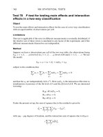
Test 78 F-test for testing main effects and interaction
effects in a two-way classification
Object
To test the main effects and interaction effects for the case of a two-way classification
with an equal number of observations per cell.
Limitations
This test is applicable if the error in different measurements is normally distributed; if
the relative size of these errors is unrelated to any factor of the experiment; and if the
different measurements themselves are independent.
Method
Suppose we have n observations per cell of the two-way table, the observations being
Y
ijk
, i = 1, 2, , p (level of A); j = 1, 2, , q (level of B) and k = 1, 2, , r. We use
the model:
Y
ijk
= µ + α
i
+ β
j
+ (αβ)
ij
+ e
ijk
subject to the conditions that

i
α

i
=

j
β
j
=

j
all j
(αβ)
ij
=

i
all i
(αβ)
ij
= 0
and that the e
ij
are independently N(0, σ
2
). Here (αβ)
ij
is the interaction effect due to
simultaneous occurrence of the ith level of A and the jth level of B. We are interested
in testing:
H
AB

: all (αβ)
ij
= 0,
H
A
: all α
i
= 0,
H
B
: all β
j
= 0.
Under the present set-up, the sum of squares due to the residual is given by
s
2
E
=

i

j

k
(Y
ijk
− Y
ij0
)
2

,
with rpq − pjq degrees of freedom, and the interaction sum of squares due to H
AB
is
r

i

j
(

αβ)
2
ij
,
GOKA: “CHAP05D” — 2006/6/10 — 17:23 — PAGE 143 — #7
THE TESTS 143
with (p − 1)(q −1) degrees of freedom, where
(

αβ)
ij
= Y
ij0
− Y
i00
− Y
0
j
0

+ Y
000
and this is also called the sum of squares due to the interaction effects.
Denoting the interaction and error mean squares by ¯s
2
AB
and ¯s
2
E
respectively. The null
hypothesis H
AB
is tested at the α level of significance by rejecting H
AB
if
¯s
2
AB
¯s
2
E
> F
(p−1)(q−1), pq(r−1); α
and failing to reject it otherwise.
For testing H
A
: a
i
= σ for all i, the restricted residual sum of squares is
s

2
1
=

i

j

k
(Y
ijk
− Y
ij0
+ Y
i00
− Y
000
)
2
= s
2
E
+ rq

i
(Y
i00
− Y
000
)

2
,
with rpq − pq + p − 1 degrees of freedom, and
s
2
A
= rq

i
(Y
i00
− Y
000
)
2
,
with p −1 degrees of freedom. With notation analogous to that for the test for H
AB
, the
test for H
A
is then performed at level α by rejecting H
A
if
¯s
2
A
¯s
2
E

> F
(p−1), pq(r−1); α
and failing to reject it otherwise. The test for H
B
is similar.
Example
An experiment is conducted in which a crop yield is compared for three different levels
of pesticide spray and three different levels of anti-fungal seed treatment. There are
four replications of the experiment at each level combination. Do the different levels
of pesticide spray and anti-fungal treatment effect crop yield and is there a significant
interaction? The ANOVA table yields F ratios that are all below the appropriate F value
from Table 3 so the experiment has yielded no significant effects and the experimenter
needs to find more successful treatments.
GOKA: “CHAP05D” — 2006/6/10 — 17:23 — PAGE 144 — #8
144 100 STATISTICAL TESTS
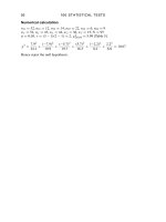
Numerical calculation
B
A I II III
1 956086
85 90 77
74 80 75
74 70 70
2 908983
80 90 70
92 91 75
82 86 72
3 706874
80 73 86
85 78 91
85 93 89

Table of means
¯
Y
ij
¯
Y
i··
1 82 75 77 78.0
2 86 89 75 83.3
3 80 78 85 81.0
¯
Y
···
¯
Y
.j.
82.7 80.7 79.0 80.8
s
2
A
= 3 × 4 ×

i
(
¯
Y
i··
−
¯
Y

···
)
2
= 3 × 4 × 14.13 = 169.56
s
2
B
= 3 × 4 ×

j
(
¯
Y
·j·
−
¯
Y
···
)
2
= 12 ×6.86 = 82.32
s
2
AB
= 4

i

j
(

¯
Y
ij·
−
¯
Y
i··
−
¯
Y
·j·
+
¯
Y
···
)
2
= 4 ×140.45 = 561.80
s
2
E
=

i

j

k
(Y
ijk

−
¯
Y
ij·
)
2
= 1830.0
ANOVA table
Source SS DF MS F ratio
A 169.56 2 84.78 1.25
B 82.32 2 41.16 0.61
AB 561.80 4 140.45 2.07
Error 1830.00 27 67.78
Critical values F
2, 27
(0.05) = 3.35 [Table 3],
F
4, 27
(0.05) = 2.73 [Table 3].
Hence we do not reject any of the three hypotheses.
GOKA: “CHAP05D” — 2006/6/10 — 17:23 — PAGE 145 — #9
THE TESTS 145
Test 79 F -test for testing main effects in a two-way
classification
Object
To test the main effects in the case of a two-way classification with unequal numbers
of observations per cell.
Limitations
This test is applicable if the error in different measurements is normally distributed; if
the relative size of these errors is unrelated to any factor of the experiment; and if the

different measurements themselves are independent.
Method
We consider the case of testing the null hypothesis
H
A
: α
i
= 0 for all i and H
B
: β
j
= 0 for all j
under additivity. Under H
A
, the model is:
Y
ijk
= µ + β
j
+ e
ijk
,
with the e
ijk
independently N(0, σ
2
). The residual sum of squares (SS) under H
A
is
s

2
2
=

i

j

k
Y
2
ijk
−

j
C
2
j
/n
·j·
with n −q degrees of freedom, where n
·j·
(µ+β
j
)+

i
n
ij
α

i
= C
j
and n
ij
is the number
of observations in the (i, j)th cell and

j
n
ij
= n
i·
and

i
n
ij
= n
·j·
the adjusted SS
due to A is
SS
A
∗
= s
2
2
− s
2

1
=

i
⎛
⎝
R
i
−

j
p
ij
C
j
⎞
⎠
ˆα
i
with p − 1 degrees of freedom, where n
i·
(µ + α
i
) +

j
n
ij
β
j

= R
i
, p
ij
= n
ij
/n
.j
.
Under additivity, the test statistic for H
A
is
SS
A
∗
s
2
1
n − p −q +1
p − 1
,
which, under H
A
, has the F-distribution with (p −1, n −p−q +1) degrees of freedom.
Similarly, the test statistic for H
B
is
SS
B
∗

s
2
1
n − p −q +1
q − 1
,
GOKA: “CHAP05D” — 2006/6/10 — 17:23 — PAGE 146 — #10
146 100 STATISTICAL TESTS
which, under H
B
, has the F-distribution with (q −1, n −p −q +1) degrees of freedom;
where SS
B
∗
=

j
(C
j
−

i
q
ij
R
i
)
ˆ
β
j

is the adjusted SS due to B, with q −1 degrees of
freedom.
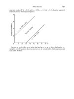
Example
Three different chelating methods (A) are used on three grades of vitamin supplement
(B). The availability of vitamin is tested byastandard timed-release method. Since some
of the tests failed there are unequal cell numbers. An appropriate analysis of variance is
conducted, so that the sums of squares are adjusted accordingly. Here chelating method
produce significantly different results but no interaction is indicated. However, Grade
of vitamin has indicated no differences.
Numerical calculation
A
B 123
Total
22 60
(126)
88 26 66 369
1 (172) (71) [0.2857]
84 23
[0.2500] [0.4286]
108 82
98 10 54
2 (308) (34) (196) 538
102 24 60
[0.3750] [0.2857] [0.4286]
108
80 20 50
3 (276) (36) (82) 394
88 16 32
[0.3750] [0.2857] [0.2857]
Total

756 141 404 1301
Note
1. Values in parentheses are the totals.
2. Values in brackets are the ratio of the number of observations divided by the column
total number of observations, e.g. the first column has 2/8 = 0.25.
T = 1301, and T
2
= observation sum of squares = 100 021
CF (correction factor) =
T
2
N
= 76 936.41
Total SS = T
2
−
T
2
N
= 23 084.59
GOKA: “CHAP05D” — 2006/6/10 — 17:23 — PAGE 147 — #11
THE TESTS 147
SS between cells =
1
2
(172)
2
+
1
3

(71)
2
+···+
1
2
(82)
2
− CF = 21 880.59
SS within cells (error) = total SS − SS between cells = 1204.00
SS
A
unadjusted =
1
8
(756)
2
+
1
7
(141)
2
+
1
7
(404)
2
− CF = 20 662.30
SS
B
unadjusted =

1
7
(369)
2
+
1
8
(538)
2
+
1
7
(394)
2
− CF = 872.23
C
11
= 7 − 2(0.2500) − 3(0.4286) − 2(0.2857) = 4.6428
C
12
=−5.0178, Q
1
= 369 − 756(0.2500) − 141(0.4286)
− 404(0.2857) = 4.145
Q
2
= 41.062, Q
3
=−45.2065, ˆα
1

= 0.8341, ˆα
2
= 5.4146, ˆα
3
=−6.2487
SS
B
adjusted = Q
1
ˆα
1
+ Q
2
ˆα
2
+ Q
3
ˆα
3
= 508.27
SS
A
adjusted = SS
B
adjusted + SS
A
unadjusted
− SS
B
unadjusted = 20 298.34

SS interaction = SS between cells −SS
B
adjusted
− SS
A
unadjusted = 710.02
ANOVA table
Source DF SS MS F ratio
SSA adjusted 2 20 298.34 10 149.17 109.58
SSB adjusted 2 508.27 254.14 2.744
Interaction AB 4 710.02 177.50 1.92
Error 13 1 204.00 92.62
Critical values F
2,13; 0.05
= 3.81 [Table 3]
F
4,13; 0.05
= 3.18 [Table 3]
The main effects of A is significantly different, whereas the main effect B and interaction
between A and B are not significant.
GOKA: “CHAP05D” — 2006/6/10 — 17:23 — PAGE 148 — #12
148 100 STATISTICAL TESTS
Test 80 F-test for nested or hierarchical classification
Object
To test for nestedness in the case of a nested or hierarchical classification.
Limitations
This test is applicable if the error in different measurements is normally distributed; if
the relative size of these errors is unrelated to any factor of the experiment; and if the
different measurements themselves are independent.
Method

In the case of a nested classification, the levels of factor B will be said to be nested with
the levels of factor A if any level of B occurs with only a single level of A. This means
that if A has p levels, then the q levels of B will be grouped into p mutually exclusive
and exhaustive groups, such that the ith group of levels of B occurs only with the ith
level of A in the observations. Here we shall only consider two-factor nesting, where
the number of levels of B associated with the ith level of A is q
i
, i.e. we consider the
case where there are

i
q
i
levels of B.
For example, consider a chemical experiment where factor A stands for the method
of analysing a chemical, there being p different methods. Factor B may represent the
different analysts, there being q
i
analysts associated with the ith method.
The jth analyst performs the n
ij
experiments allotted to him. The corresponding fixed
effects model is:
Y
ijk
= µ + α
i
+ β
ij
+ e

ijk
, i = 1, 2, , p; j = 1, 2, , q
i
;
k = 1, 2, , n
ij
,
p

i=l
n
i
α
i
=

j
all j
n
ij
β
j
= 0
n
i
=

j
n
ij

, n =

i
n
i
and e
ijk
are independently N(0, σ
2
).
We are interested in testing H
A
: α
i
= 0, for all i, and H
B
: β
ij
= 0, for all i, j.
The residual sum of squares is given by
s
2
E
=

i

j

k

(Y
ijk
− Y
ij0
)
2
with

ij
(n
ij
−1) degrees of freedom; the sums of squares due respectively to A and B
are
s
2
A
=

i
n
i
(Y
i00
− Y
000
)
2
GOKA: “CHAP05D” — 2006/6/10 — 17:23 — PAGE 149 — #13
THE TESTS 149
with p − 1 degrees of freedom, and

s
2
B
=

i

j
n
ij
(Y
ij0
− Y
i00
)
with

i
(q
i
− 1) degrees of freedom.
To perform the tests for H
A
and H
B
we first require the mean squares, ¯s
2
E
, ¯s
2

A
and ¯s
2
B
,
corresponding to these sums of squares; we then calculate ¯s
2
A
/¯s
2
E
to test H
A
and ¯s
2
B
/¯s
2
E
to
test H
B
, each of which, under the respective null hypothesis, follows the F-distribution
with appropriate degrees of freedom.
Nested models are frequently used in sample survey investigations.
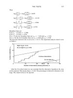
Example
An educational researcher wishes to establish the relative contribution from the teachers
and schools towards pupils’ reading scores. She has collected data relating to twelve
teachers (three in each of four schools). The analysis of variance table produces an F
ratio of 1.46 which is less than the critical value of 2.10 from Table 3. So the differences

between teachers are not significant. The differences between schools are, however,
significant since the calculated F ratio of 6.47 is greater than the critical value of 4.07.
Why the schools should be different is another question.
Numerical calculation
Scores of pupils from three teachers in each of four schools are shown in the following
table.
Schools
I II III IV
Teacher Teacher Teacher Teacher
123123123123
44 39 39 51 48 44 46 45 43 42 45 39
41 37 36 49 43 43 43 40 41 39 40 38
39 35 33 45 42 42 41 38 39 38 37 35
36 35 31 44 40 39 40 38 37 36 37 35
35 34 28 40 37 37 36 35 34 34 32 35
32 30 26 40 34 36 34 34 33 31 32 29
Teacher total 227 210 193 269 244 241 240 230 227 220 223 211
Mean 37.83 35.0 32.17 44.83 40.67 40.17 40.0 38.33 37.83 36.67 37.17 35.17
School total 630 754 697 654 2735
Mean 35.00 41.89 38.72 36.34
T = 2735
CF (correction factor) =
2735
2
72
= 103 892.01
Total sum of squares = 105 637.00 − 103 892.01 = 1744.99
GOKA: “CHAP05D” — 2006/6/10 — 17:23 — PAGE 150 — #14
150 100 STATISTICAL TESTS
Between-schools sum of squares

=
630
2
18
+
754
2
18
+
697
2
18
+
654
2
18
− CF = 493.60
Between teachers (within school) sum of squares
=
227
2
6
+
210
2
6
+
193
2
6

+
630
2
18
+ similar terms for schools II, III and IV = 203.55
Within-group sum of squares = 1744.99 −493.60 − 203.55 = 1047.84.
ANOVA table
DF SS Mean square
Schools 3 493.60 164.53
Teachers within school 8 203.55 25.44
Pupils within teachers 60 1047.84 17.46
Total 71 1744.99
Teacher differences:
F =
25.44
17.46
= 1.46
Critical value F
8,60; 0.05
= 2.10 [Table 3].
The calculated value is less than the critical value.
Hence the differences between teachers are not significant.
School differences:
F =
164.53
25.44
= 6.47
Critical value F
3,8; 0.05
= 4.07 [Table 3].

The calculated value is greater than the critical value.
Hence the differences between schools are significant.
GOKA: “CHAP05D” — 2006/6/10 — 17:23 — PAGE 151 — #15
THE TESTS 151
Test 81 F -test for testing regression
Object
To test the presence of regression of variable Y on the observed value X.
Limitations
For given X, the Y s are normally and independently distributed. The error terms are
normally and independently distributed with mean zero.
Method
Suppose, corresponding to each value X
i
(i = 1, 2, , p) of the independent random
variable X, we have a corresponding array of observations Y
ij
( j = 1, 2, , n
i
) on the
dependent variable Y . Using the model:
Y
ij
= µ
i
+ e
ij
, i = 1, 2, , p, j = 1, 2, , n
i
,
where the e

ij
are independently N (0, σ
2
), we are interested in testing H
0
: all µ
i
are
equal, against H
1
: not all µ
i
are equal. ‘H
0
is true’ implies the absence of regression of
Y on X. Then the sums of squares are given by
s
2
B
=

i
n
i
(Y
i0
− Y
00
)
2

, s
2
E
=

i

j
(Y
ij
− Y
i0
)
2
.
Denoting the corresponding mean squares by ¯s
2
B
and ¯s
2
E
respectively, then, under H
0
,
F =¯s
2
B
/¯s
2
E

follows the F-distribution with (p − 1, n − p) degrees of freedom.
Example
It is desired to test for the presence of regression (i.e. non-zero slope) in comparing an
independent variable X, with a dependent variable Y.
A small-scale experiment is set up to measure perceptions on a simple dimension
(Y) to a visual stimulus (X). The results test for the presence of a regression of Y on X.
The experiment is repeated three times at two levels of X.
Since the calculated F value of 24 is larger than the critical F value from Table 3,
the null hypothesis is rejected, indicating the presence of regression.
Numerical calculation
Y
ij
X
1
X
2
123
756
n
1
= 3, where Y
i0
=
n
i

j=1
Y
ij
n

i
, i = 1, 2, , p
n
2
= 3, and Y
00
=

i

j
Y
ij
n
, n =

n
i
GOKA: “CHAP05D” — 2006/6/10 — 17:23 — PAGE 152 — #16
152 100 STATISTICAL TESTS
Hence Y
10
=
1 + 2 + 3
3
= 2, Y
20
=
7 + 5 + 6
3

= 6,
Y
00
=
1 + 2 + 3 +7 +5 + 6
6
= 4
s
2
B
= 3(2 −4)
2
+ 3(6 −4)
2
= 24
s
2
E
= (1 − 2)
2
+ (2 −2)
2
+ (3 −2)
2
+ (7 −6)
2
+ (5 −6)
2
+ (6 −6)
2

= 4
¯s
2
B
= 24/1 = 24, ¯s
2
E
= 4/4 = 1, F = 24/1 = 24
Critical value F
1,4; 0.05
= 7.71 [Table 3].
Hence reject the null hypothesis, indicating the presence of regression.
GOKA: “CHAP05D” — 2006/6/10 — 17:23 — PAGE 153 — #17
THE TESTS 153
Test 82 F -test for testing linearity of regression
Object
To test the linearity of regression between an X variable and a Y variable.
Limitations
For given X, the Y s are normally and independently distributed. The error terms are
normally and independently distributed with mean zero.
Method
Once the relationship between X and Y is established using Test 81, we would further
like to know whether the regression is linear or not. Under the same set-up as Test 81,
we are interested in testing:
H
0
: µ
i
= α + βX
i

, i = 1, 2, , n,
Under H
0
,
s
2
E
=

i
(y
i
−¯y) − b
2

i
n
i
(x
i
−¯x)
2
,
with n − 2 degrees of freedom, and the sum of squares due to regression
s
2
R
= b
2


i
n
i
(x
i
−¯x)
2
,
with 1 degree of freedom. The ratio of mean squares
F =¯s
2
R
/¯s
2
E
is used to test H
0
with (1, n −2) degrees of freedom.
Example
In a chemical reaction the quantity of plastic polymer (Y ) is measured at each of four
levels of an enzyme additive (X). The experiment is repeated three times at each level
of X to enable a test of linearity of regression to be performed.
The data produce an F value of 105.80 and this is compared with the critical F value
of 4.96 from Table 3. Since the critical value is exceeded we conclude that there is a
significant regression.
Numerical calculation
i 123456789101112
x
i
150 150 150 200 200 200 250 250 250 300 300 300

y
i
77.4 76.7 78.2 84.1 84.5 83.7 88.9 89.2 89.7 94.8 94.7 95.9
n = 12, n − 2 = 10. For β = 0, test H
0
: β = 0 against H
1
: β = 0
GOKA: “CHAP05D” — 2006/6/10 — 17:23 — PAGE 154 — #18
154 100 STATISTICAL TESTS
The total sum of squares is

y
2
i
−


y
i

2

n = 513.1167,
and
s
2
R
= b



x
i
y
i
−
1
n

x
i
y
i

2

x
2
i
−
1
n
(x
i
)
2
= 509.10,
s
2
E

= 4.0117, ¯s
2
R
= 42.425, ¯s
2
E
= 0.401, F = 105.80
Critical value F
1,10; 0.05
= 4.96 [Table 3].
Hence reject the null hypothesis and conclude that β = 0.
GOKA: “CHAP05D” — 2006/6/10 — 17:23 — PAGE 155 — #19
THE TESTS 155
Test 83 Z-test for the uncertainty of events
Object
To test the significance of the reduction of uncertainty of past events.
Limitations
Unlike sequential analyses, this test procedure requires a probability distribution of a
variable.
Method
It is well known that the reduction of uncertainty by knowledge of past events is the
basic concept of sequential analysis. The purpose here is to test the significance of this
reduction of uncertainty using the statistic
Z =
P (B
+k
|A) − P(B)

P (B)[1 − P(B)][1 − P(A)]
(n − k)P(A)

where P(A) =probability of A, P (B) =probability of B and P(B
+k
|A) =P(B|A) at lag k.
Example
An economic researcher wishes to test for the reduction of uncertainty of past events.
He notes that following a financial market crash (event A) a particular economic index
rises (event B). His test statistic of Z = 2.20 is greater than the tabulated value of
1.96 from Table 1. This is a significant result allowing him to claim a reduction of
uncertainty for events A and B.
Numerical calculation
Consider a sequence of A and B: AA BA BA BB AB AB
n = 12, k = 1, P(A) =
6
12
= 0.5, P(B) =
6
12
= 0.5
We note that A occurs six times and that of these six times B occurs immediately after
A five times. Given that A just occurred we have
P (B|A) at lag one = P(B
+1
|A) =
5
6
= 0.83.
Therefore the test statistic is
Z =
0.83 − 0.50


0.50(1 −0.50)(1 − 0.50)
(12 −1)(0.50)
= 2.20.
The critical value at α = 0.05 is 1.96 [Table 1].
The calculated value is greater than the critical value.
Hence it is significant.
GOKA: “CHAP05D” — 2006/6/10 — 17:23 — PAGE 156 — #20
156 100 STATISTICAL TESTS
Test 84 Z-test for comparing sequential
contingencies across two groups using the
‘log odds ratio’
Object
To test the significance of the difference in sequential connections across groups.
Limitations
This test is applicable when a logit transformation can be used and 2 × 2 contingency
tables are available.
Method
Consider a person’s antecedent behaviour (W
t
) taking one of the two values:
W
t
=

1 for negative effect
0 for positive effect.
Let us use H
t
+ 1, a similar notation, for the spouse’s consequent behaviour. A funda-
mental distinction may be made between measures of association in contingency tables

which are either sensitive or insensitive to the marginal (row) totals. A measure that
is invariant to the marginal total is provided by the so-called logit transformation. The
logit is defined by:
logit (P) = log
e
P
1 − P
.
We can now define a statistic β as follows:
β = logit [P
r
(H
t+k
= 1|W
t
= 1)]−logit[P
r
(H
t+k
= 1|W
t
= 0)].
Hence β is known as the logarithm of the ‘odds ratio’ which is the cross product ratio in
a2×2 contingency table, i.e. if we have a table in which first row is (a, b) and second
row is (c, d) then
β = log

ad
bc


.
In order to test whether β is different across groups we use the statistic
Z =
β
1
− β
2



1
f
i

where f
i
is the frequency in the ith cell and Z is the standard normal variate, i.e. N(0, 1).
GOKA: “CHAP05D” — 2006/6/10 — 17:23 — PAGE 157 — #21
THE TESTS 157
Example
A social researcher wishes to test a hypothesis concerning the behaviour of adult
couples. She compares a man’s behaviour with a consequent spouse’s behaviour for
couples in financial distress and for those not in financial distress. A log-odds ratio test
is used. In this case the Z value of 1.493 is less than the critical value of 1.96 from
Table 1. She concludes that there is insufficient evidence to suggest financial distress
affects couples’ behaviour in the way she hypothesizes.
Numerical calculation
Distressed couples Non-distressed couples
W
t+1

W
t+1
H
t
101 0
1 76 100 80 63
0 79 200 43 39
β
1
= log
e
76 × 200
79 × 100
= 0.654; β
2
= log
e
80 ×39
43 × 63
= 0.141
Z =
0.654 − 0.141

1
76
+
1
79
+
1

100
+
1
200
+
1
80
+
1
43
+
1
63
+
1
39
= 1.493
The critical value at α = 0.05 is 1.96 [Table 1].
The calculated value is less than the critical value.
Hence it is not significant and the null hypothesis (that β is not different across groups)
cannot be rejected.
GOKA: “CHAP05D” — 2006/6/10 — 17:23 — PAGE 158 — #22
158 100 STATISTICAL TESTS
Test 85 F -test for testing the coefficient of multiple
regression
Object
A multiple linear regression model is used in order to test whether the population value
of each multiple regression coefficient is zero.
Limitations
This test is applicable if the observations are independent and the error term is normally

distributed with mean zero.
Method
Let X
1
, X
2
, , X
k
be k independent variables and X
1i
, X
2i
, , X
ki
be their fixed values,
corresponding to dependent variables Y
i
. We consider the model:
Y
i
= β
0
+ β
1
X

1i
+···+β
k
X


ki
+ e
i
where X

ji
= X
ji
−
¯
X
j
and the e
i
are independently N(0, σ
2
).
We are interested in testing whether the population value of each multiple regression
coefficient is zero. We want to test:
H
0
: β
1
= β
2
=···=β
k
= 0 against H
1

: not all β
k
= 0
for k = 1, 2, , p −1, where p is the number of parameters. The error sum of squares
is
s
2
E
=

i
(Y
i
−
¯
Y)
2
−

j
b
j

i
Y
i
X

ji
with n − k − 1 degrees of freedom, where b

j
is the least-squares estimator of β
j
.
The sum of squares due to H
0
is
s
2
H
=

j
b
j

i
Y
i
X

ji
with k degrees of freedom. Denoting the corresponding mean squares by ¯s
2
E
and ¯s
2
H
respectively, then, under H
0

, F =¯s
2
H
/¯s
2
E
follows the F-distribution with (k, n − k − 1)
degrees of freedom and can be used for testing H
0
.
The appropriate decision rule is: if the calculated F
 F
p−1, n−p; 0.05
, do not reject
H
0
; if the calculated F > F
p−1, n−p; 0.05
, reject H
0
.
Example
In an investigation of the strength of concrete (Y ), a number of variables were measured
(X
1
, X
2
, , X
k
) and a multiple regression analysis performed. The global F test is a

GOKA: “CHAP05D” — 2006/6/10 — 17:23 — PAGE 159 — #23
THE TESTS 159
test of whether any of the X variables is significant (i.e. any of the β
i
coefficients,
i = 1, , k are non-zero).
The calculated F value of 334.35 is greater thanthetabulated F value of 3.81[Table3].
So at least one of the X variables is useful in the prediction of Y.
Numerical calculation
n = 16, p = 3, ν = p −1, ν
2
= n − p
Critical value F
2, 13; 0.05
= 3.81 [Table 3].
From the computer output of a certain set of data
¯s
2
H
= 96.74439, ¯s
2
E
= 0.28935
F = 96.74439/0.28935 = 334.35
Hence reject the null hypothesis.
GOKA: “CHAP05D” — 2006/6/10 — 17:23 — PAGE 160 — #24
160 100 STATISTICAL TESTS
Test 86 F -test for variance of a random effects model
Object
To test for variance in a balanced random effects model of random variables.

Limitations
This test is applicable if the random variables are independently and normally
distributed with mean zero.
Method
Let the random variable Y
ij···m
for a balanced case be such that:
Y
ij···m
= µ + a
i
+ b
ij
+ c
ijk
+···+e
ijk···m
where µ is a constant and the random variables a
i
, b
ij
, c
ijk
, , e
ijk···m
are completely
independent and a
i
∼ N(0, σ
2

a
), , b
ij
∼ N(0, σ
2
b
), c
ijk
∼ N(0, σ
2
c
), , e
ijk···m
∼
N(0, σ
2
e
).
Then the test for H
0
= σ
2
i
= σ
2
j
(i = j) against H
1
= σ
2

i
>σ
2
j
is given by s
2
i
/s
2
j
which is distributed as (σ
2
i
/σ
2
j
)F and follows the F-distribution with (f
i
, f
j
) degrees of
freedom. Here s
2
i
and s
2
j
are the estimates of σ
2
i

and σ
2
j
.
Example
An electronic engineer wishes to test for company and sample electrical static dif-
ferences for a component used in a special process. He selects three companies at
random and also two samples. He collects four measurements of static from selected
components. Are the companies all the same with respect to electrical resistance of
the particular component? His analysis of variance calculation produces an F value of
1.279. He compares this with the tabulated F value of 9.55 [Table 3] and concludes
that there is no evidence to suggest company differences.
Numerical calculation
s
2
1
= 5.69, s
2
2
= 4.45, f
1
= 2, f
2
= 3
H
0
: σ
2
1
= σ

2
2
; H
1
: σ
2
1
>σ
2
2
F =
s
2
1
s
2
2
=
5.69
4.45
= 1.279
Critical value F
2,3; 0.05
= 9.55 [Table 3]
Hence we do not reject the null hypothesis H
0
.
f
1
= n

1
− 1 Here: n
1
= 3, n
2
= 2
f
2
= 2n
2
− 1
GOKA: “CHAP05D” — 2006/6/10 — 17:23 — PAGE 161 — #25
THE TESTS 161
Test 87 F -test for factors A and B and an interaction
effect
Object
To test for the homogeneity of factors A and B and the absence of an interaction effect.
Limitations
This test is applicable if the random variables and interaction effects are jointly normal
with mean zero and the error terms are independently normally distributed with mean
zero.
Method
Let the factor having fixed levels be labelled A and represented by the columns of the
table and let the randomly sampled factor be B and represented by the rows. Let
Y
ijk
= µ + α
i
+ b
k

+ c
jk
+ e
ijk
where
α
i
is the fixed effect of the treatment indicated by the column i;
b
k
= random variable associated with the kth row;
c
jk
= random interaction effect operating on the ( j, k)th cell; and
e
ijk
= random error associated with observation i in the ( j, k)th cell.
We make the following assumptions:
1. b
k
and c
jk
are jointly normal with mean zero and with variance σ
2
B
and σ
2
AB
,
respectively;

2. e
ijk
are normally distributed with mean zero and variance σ
2
E
;
3. e
ijk
are independent of b
k
and c
jk
;
4. e
ijk
are independent of each other.
Denoting the column, interaction, row and error mean squares by ¯s
2
C
, ¯s
2
I
, ¯s
2
R
and ¯s
2
E
respectively, then ¯s
2

C
/¯s
2
I
∼ F
c−1,(r−1)(c−1)
provides an appropriate test for the column
effects, i.e. H
0
: σ
2
A
= 0; ¯s
2
R
/¯s
2
E
∼ F
r−1, rc(n−1)
provides a test for H
0
: σ
2
B
= 0; and
¯s
2
I
/¯s

2
E
∼ F
(r−1)(c−1),r(n−1)
provides a test for H
0
: σ
2
AB
= 0.
Example
An educational researcher has collected data on pupils’ performance in relation to three
tasks; six classes are compared. The analysis of variance suggests that neither classroom
nor task factors is significant but their interaction is significant.
GOKA: “CHAP05D” — 2006/6/10 — 17:23 — PAGE 162 — #26
162 100 STATISTICAL TESTS
Numerical calculation
In the following table the values are a combination of classroom and task and represent
the independent performance of two subjects in each cell.
Tasks
Classroom I II III Total
1 7.8 11.1 11.7
(16.5) (23.1) (21.7) 61.3
8.7 12.0 10.0
2 8.0 11.3 9.8
(17.2) (21.9) (21.7) 60.8
9.2 10.6 11.9
3 4.0 9.8 11.7
(10.9) (19.9) (24.3) 55.1
6.9 10.1 12.6

4 10.3 11.4 7.9
(19.7) (21.9) (16.0) 57.6
9.4 10.5 8.1
5 9.3 13.0 8.3
(19.9) (24.7) (16.2) 60.8
10.6 11.7 7.9
6 9.5 12.2 8.6
(19.3) (24.5) (19.1) 62.9
9.8 12.3 10.5
Total 103.5 136.0 119.0 358.5
CF (correction factor) = 358.5
2
/36 = 3570.0625
TSS = 7.8
2
+···+10.5
2
− (3570.0625) = 123.57
The sums of squares are given by
s
2
C
=
(103.5)
2
+ (136.0)
2
+ (119.0)
2
12

− CF = 44.04
s
2
R
=
61.3
2
+···+62.9
2
6
− CF = 6.80
s
2
E
= 7.8
2
+···+10.5
2
−
16.5
2
+···+19.1
2
2
= 14.54
s
2
I
= 123.57 − 44.04 − 6.8 −14.54 = 58.19
GOKA: “CHAP05D” — 2006/6/10 — 17:23 — PAGE 163 — #27

THE TESTS 163
ANOVA table
Source DF SS MS F
Column 2 44.04 22.02 3.78
Row 5 6.80 1.36 1.68
Interaction 10 58.19 5.82 7.19
Error 18 14.54 0.81
Total 35 123.57
Critical values F
10,18;0.05
= 2.41 [Table 3]
F
2,10; 0.05
= 4.10
F
5,18; 0.05
= 2.77
Hence H
0
: σ
AB
= 0 is rejected.
H
0
: σ
2
A
= 0 is not rejected.
H
0

: σ
2
B
= 0 is not rejected.
GOKA: “CHAP05D” — 2006/6/10 — 17:23 — PAGE 164 — #28
164 100 STATISTICAL TESTS
Test 88 Likelihood ratio test for the parameter of
a rectangular population
Object
To test for one of the parameters of a rectangular population with probability density
function
f
0
(X) =
⎧
⎨
⎩
1
2β
, α −β
 X  α +β
0, otherwise.
Limitations
This test is applicable if the observations are a random sample from a rectangular
distribution.
Method
Let X
1
, X
2

, , X
n
be a random sample from the above rectangular population. We are
interested in testing H
0
: α = 0 against H
1
: α = 0. Then, the likelihood ratio test
criterion for testing H
0
is:
λ =

X
(n)
− X
(1)
2Z

n
=

R
2Z

n
,
where R is the sample range and Z = max[−X
(1)
, X

(n)
]. Then the asymptotic
distribution of 2 log
e
λ is χ
2
2
.
Example
An electronic component test profile follows a rectangular distribution at stepped input
levels. An electronic engineer wishes to test a particular component type and collects
his data. He uses a likelihood ratio test. He obtains a value of his test statistic of −4.2809
and compares this with his tabulated value. He thus rejects the null hypothesis that one
parameter is zero.
Numerical calculation
Consider (−0.2, −0.3, −0.4, 0.4, 0.3, 0.5) as a random sample from a rectangular
distribution. Here,
n = 6
R = 0.5 −(−0.2) = 0.7, Z = max[0.4, 0.5]=0.5
λ =

R
2Z

6
= (0.7)
6
= 0.1176, 2 log
e
λ =−4.2809

Critical value χ
2
2; 0.05
= 5.99 [Table 5].
Hence we reject the null hypothesis that α = 0.
GOKA: “CHAP05D” — 2006/6/10 — 17:23 — PAGE 165 — #29
THE TESTS 165
Test 89 Uniformly most powerful test for the
parameter of an exponential population
Object
To test the parameter (θ) of the exponential population with probability density function
f (X, θ) = θe
−θX
, X > 0.
Limitations
The test is applicable if the observations are a random sample from an exponential
distribution.
Method
Let X
1
, X
2
, , X
n
be a random sample from an exponential distribution with parame-
ter θ. Let our null hypothesis be H
0
: θ = θ
0
against the alternative H

1
: θ = θ
1
(θ
1
= θ
0
).
Case (a) θ
1
>θ
0
: The most powerful critical region is given by:
W
0
=

X =

i
X
i
 χ
2
2n;1−α
/2θ
0

.
Since W

0
is independent of θ
1
,soW
0
is uniformly most powerful for testing H
0
: θ = θ
0
against H
1
: θ>θ
0
.
Case (b) θ
1
<θ
0
: The most powerful critical region is given by:
W
1
=

X =

X
i
>χ
2
2n; α

/2θ
0

.
Again W
1
is independent of θ
1
and so it is also uniformly most powerful for testing
H
0
: θ = θ
0
against H
1
: θ<θ
0
.
Example
An electronic component is tested for an exponential failure distribution with a given
parameter. The given example produces a critical region for the test of parameter equal
to 1 against the alternative hypothesis that it equals 2.
Numerical calculation
Let us consider a sample of size 2 from the population f (X
1
θ) = θe
−θX
, X > 0.
Consider testing H
0

: θ = 1 against H
1
: θ = 2, i.e. θ>θ
0
. The critical region is
W =

X


X
i
 χ
2
0.95,4/2

=

X


X
i
 0.71/2

[Table 5]
=

X



X
i
 0.36

GOKA: “CHAP05D” — 2006/6/10 — 17:23 — PAGE 166 — #30
166 100 STATISTICAL TESTS
Test 90 Sequential test for the parameter of
a Bernoulli population
Object
To test the parameter of the Bernoulli population by the sequential method.
Limitations
This test is applicable if the observations are independent and identically follow the
Bernoulli distribution.
Method
Let X
1
, X
2
, , X
m
be independent and identically distributed random variables having
the distribution with probability density function (PDF)
f
(x)
0
=

θ
x

(1 − θ)
1−x
, X = 0, 1
0, otherwise.
where 0 <θ<1. We want to test H
0
: θ = θ
0
against H
1
: θ = θ
1
.
We fail to reject H
0
if S
m
 a
m
, and we reject H
0
if S
m
 r
m
. We continue sampling,
i.e. taking observations, if a
m
< S
m

< r
m
, where S
m
=

m
i=1
X
i
and
a
m
=
log
β
1 − α
log

θ
1
θ
0

− log

1 − θ
1
1 − θ
0


+
m log

1 − θ
0
1 − θ
1

log

θ
1
θ
0

− log

1 − θ
1
1 − θ
0

r
m
=
log
1 − β
α
log


θ
1
θ
0

− log

1 − θ
1
1 − θ
0

+
m log

1 − θ
0
1 − θ
1

log

θ
1
θ
0

− log


1 − θ
1
1 − θ
0

.
Example
Same as Numerical calculation.
Numerical calculation
While dealing with the sampling of manufactured products, θ may be looked upon as
the true proportion of defectives under a new production process. A manufacturer may
be willing to adopt the new process if θ
 θ
0
and will reject it if θ  θ
1
and he may
not be decisive if θ
0
<θ<θ
1
. To reach a decision, he may use a sequential sampling
plan, taking one item at each stage and at random. Here S
m
will be the number of
defectives up to the mth stage, a
m
the corresponding acceptance number and r
m
the