Biosignal and Biomedical Image Processing MATLAB-Based Applications Muya phần 8 pptx

PCA and ICA 267
F
IGURE
9.13 Scree plot of eigenvalues from the data set of Figure 9.12. Note the
shape break at N = 3, indicating that there are only three independent variables in
the data set of five waveforms. Hence, the ICA algorithm will be requested to
search for only three components.
%
% Do PCA and plot Eigenvalues
figure;
[U,S,pc]= svd(X,0); % Use single value decomposition
eigen = diag(S).v2; % Get the eigenvalues
plot(eigen,’k’); % Scree plot
labels and title
%
nu_ICA = input(’Enter the number of independent components’);
% Compute ICA
W = jadeR(X,nu_ICA); % Determine the mixing matrix
ic = (W * X)’; % Determine the IC’s from the
% mixing matrix
figure; % Plot independent components
plot(t,ic(:,1)-4,’k’,t,ic(:,2),’k’,t,ic(:,3)؉4,’k’);
labels and title
The original source signals are shown in Figure 9.12. These are mixed
together in different proportions to produce the five signals shown in Figure
9.14. The Scree plot of the eigenvalues obtained from the five-variable data set
does show a marked break at 3 suggesting that there, in fact, only three separate
components, Figure 9.13. Applying ICA to the five-variable mixture in Figure
TLFeBOOK
F
IGURE

9.14 Five signals created by mixing three different waveforms and noise.
ICA was applied to this data set to recover the original signals. The results of
applying ICA to this data set are seen in Figure 9.15.
268
TLFeBOOK
PCA and ICA 269
F
IGURE
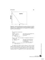
9.15 The three independent components found by ICA in Example 9.3.
Note that these are nearly identical to the original, unmixed components. The
presence of a small amount of noise does not appear to hinder the algorithm.
9.14 recovers the original source signals as shown in Figure 9.15. This figure
dramatically demonstrates the ability of this approach to recover the original
signals even in the presence of modest noise. ICA has been applied to biosignals
to estimate the underlying sources in an multi-lead EEG signal, to improve the
detection of active neural areas in functional magnetic resonance imaging, and
to uncover the underlying neural control components in an eye movement motor
control system. Given the power of the approach, many other applications are
sure to follow.
TLFeBOOK
270 Chapter 9
PROBLEMS
1. Load the two-variable data set, X, contained in file
p1_data
. Assume for
plotting that the sample frequency is 500 Hz. While you are not given the di-
mensions or orientation of the data set, you can assume the number of time
samples is much greater than the number of measured signals.
(A) Rotate these data by an angle entered through the keyboard and output the
covariance (from the covariance matrix) after each rotation. Use the function

rotate
to do the rotation. See comments in the function for details. Continue
to rotate the data set manually until the covariances are very small (less than
10
-4
). Plot the rotated and unrotated variables as a scatter plot and output their
variances (also from covariance matrix). The variances will be the eigenvalues
found by PCA and the rotated data the principal components.
(B) Now apply PCA using the approach given in Example 9.1 and compare the
scatter plots with the manually rotated data. Compare the variances of the princi-
pal components from PCA (which can be obtained from the eigenvalues) with
the variances obtained by manual rotation in (A) above.
2. Load the multi-variable data set, X, contained in file
p2_data
. Make the
same assumptions with regard to sampling frequency and data set size as in
Problem 1 above.
(A) Determine the actual dimension of the data using PCA and the scree plot.
(B) Perform an ICA analysis using either the Jade or FastICA algorithm limiting
the number of components determined from the scree plot. Plot independent
components.
TLFeBOOK
10
Fundamentals of Image Processing:
MATLAB Image Processing Toolbox
IMAGE PROCESSING BASICS: MATLAB IMAGE FORMATS
Images can be treated as two-dimensional data, and many of the signal process-
ing approaches presented in the previous chapters are equally applicable to im-
ages: some can be directly applied to image data while others require some
modification to account for the two (or more) data dimensions. For example,

both PCA and ICA have been applied to image data treating the two-dimen-
sional image as a single extended waveform. Other signal processing methods
including Fourier transformation, convolution, and digital filtering are applied to
images using two-dimensional extensions. Two-dimensional images are usually
represented by two-dimensional data arrays, and MATLAB follows this tradi-
tion;* however, MATLAB offers a variety of data formats in addition to the
standard format used by most MATLAB operations. Three-dimensional images
can be constructed using multiple two-dimensional representations, but these
multiple arrays are sometimes treated as a single volume image.
General Image Formats: Image Array Indexing
Irrespective of the image format or encoding scheme, an image is always repre-
sented in one, or more, two dimensional arrays,
I(m,n)
. Each element of the
*Actually, MATLAB considers image data arrays to be three-dimensional, as described later in this
chapter.
271
TLFeBOOK
272 Chapter 10
variable,
I
, represents a single picture element, or pixel. (If the image is being
treated as a volume, then the element, which now represents an elemental vol-
ume, is termed a voxel.) The most convenient indexing protocol follows the
traditional matrix notation, with the horizontal pixel locations indexed left to
right by the second integer,
n
, and the vertical locations indexed top to bottom
by the first integer
m

(Figure 10.1). This indexing protocol is termed pixel coor-
dinates by MATLAB. A possible source of confusion with this protocol is that
the vertical axis positions increase from top to bottom and also that the second
integer references the horizontal axis, the opposite of conventional graphs.
MATLAB also offers another indexing protocol that accepts non-integer
indexes. In this protocol, termed spatial coordinates, the pixel is considered to
be a square patch, the center of which has an integer value. In the default coordi-
nate system, the center of the upper left-hand pixel still has a reference of (1,1),
but the upper left-hand corner of this pixel has coordinates of (0.5,0.5) (see
Figure 10.2). In this spatial coordinate system, the locations of image coordi-
nates are positions on a (discrete) plane and are described by general variables
x and y. The are two sources of potential confusion with this system. As with
the pixel coordinate system, the vertical axis increases downward. In addition,
the positions of the vertical and horizontal indexes (now better though of as
coordinates) are switched: the horizontal index is first, followed by the vertical
coordinate, as with conventional x,y coordinate references. In the default spatial
coordinate system, integer coordinates correspond with their pixel coordinates,
remembering the position swap, so that
I(5,4)
in pixel coordinates references
the same pixel as
I(4.0,5.0)
in spatial coordinates. Most routines expect a
specific pixel coordinate system and produce outputs in that system. Examples
of spatial coordinates are found primarily in the spatial transformation routines
described in the next chapter.
It is possible to change the baseline reference in the spatial coordinate
F
IGURE
10.1 Indexing format for MATLAB images using the pixel coordinate sys-

tem. This indexing protocol follows the standard matrix notation.
TLFeBOOK
Fundamentals of Image Processing 273
F
IGURE
10.2 Indexing in the spatial coordinate system.
system as certain commands allow you to redefine the coordinates of the refer-
ence corner. This option is described in context with related commands.
Data Classes: Intensity Coding Schemes
There are four different data classes, or encoding schemes, used by MATLAB
for image representation. Moreover, each of these data classes can store the data
in a number of different formats. This variety reflects the variety in image types
(color, grayscale, and black and white), and the desire to represent images as
efficiently as possible in terms of memory storage. The efficient use of memory
storage is motivated by the fact that images often require a large numbers of
array locations: an image of 400 by 600 pixels will require 240,000 data points,
each of which will need one or more bytes depending of the data format.
The four different image classes or encoding schemes are: indexed images,
RGB images, intensity images, and binary images. The first two classes are used
to store color images. In indexed images, the pixel values are, themselves, in-
dexes to a table that maps the index value to a color value. While this is an
efficient way to store color images, the data sets do not lend themselves to
arithmetic operations (and, hence, most image processing operations) since the
results do not always produce meaningful images. Indexed images also need an
associated matrix variable that contains the colormap , and this map variable
needs to accompany the image variable in many operations. Colormaps are N
by 3 matrices that function as lookup tables. The indexed data variable points
to a particular row in the map and the three columns associated with that row
TLFeBOOK
274 Chapter 10

contain the intensity of the colors red, green, and blue. The values of the three
columns range between 0 and 1 where 0 is the absence of the related color and
1 is the strongest intensity of that color. MATLAB convention suggests that
indexed arrays use variable names beginning in
x
(or simply
x
) and the sug-
gested name for the colormap is
map
. While indexed variables are not very
useful in image processing operations, they provide a compact method of storing
color images, and can produce effective displays. They also provide a conve-
nient and flexible method for colorizing grayscale data to produce a pseudocolor
image.
The MATLAB Image Processing Toolbox provides a number of useful
prepackaged colormaps. These colormaps can implemented with any number of
rows, but the default is 64 rows. Hence, if any of these standard colormaps are
used with the default value, the indexed data should be scaled to range between
0 and 64 to prevent saturation. An example of the application of a MATLAB
colormap is given in Example 10.3. An extension of that example demonstrates
methods for colorizing grayscale data using a colormap.
The other method for coding color image is the RGB coding scheme in
which three different, but associated arrays are used to indicate the intensity of
the three color components of the image: red, green, or blue. This coding
scheme produces what is know as a truecolor image. As with the encoding used
in indexed data, the larger the pixel value, the brighter the respective color. In
this coding scheme, each of the color components can be operated on separately.
Obviously, this color coding scheme will use more memory than indexed im-
ages, but this may be unavoidable if extensive processing is to be done on a

color image. By MATLAB convention the variable name
RGB
, or something
similar, is used for variables of this data class. Note that these variables are
actually three-dimensional arrays having dimensions N by M by 3. While we
have not used such three dimensional arrays thus far, they are fully supported
by MATLAB. These arrays are indexed as
RGB(n,m,i)
where
i
= 1,2,3. In fact,
all image variables are conceptualized in MATLAB as three-dimensional arrays,
except that for non-RGB images the third dimension is simply 1.
Grayscale images are stored as intensity class images where the pixel
value represents the brightness or grayscale value of the image at that point.
MATLAB convention suggests variable names beginning with
I
for variables
in class intensity. If an image is only black or white (not intermediate grays),
then the binary coding scheme can be used where the representative array is a
logical array containing either 0’s or 1’s. MATLAB convention is to use
BW
for
variable names in the binary class. A common problem working with binary
images is the failure to define the array as logical which would cause the image
variable to be misinterpreted by the display routine. Binary class variables can
be specified as logical (set the logical flag associated with the array) using the
command
BW = logical(A)
, assuming

A
consists of only zeros and ones. A
logical array can be converted to a standard array using the unary plus operator:
TLFeBOOK
Fundamentals of Image Processing 275
A
=
؉BW
. Since all binary images are of the form “logical,” it is possible to
check if a variable is logical using the routine:
isa(I, ’logical’)
; which will
return a1 if true and zero otherwise.
Data Formats
In an effort to further reduce image storage requirements, MATLAB provides
three different data formats for most of the classes mentioned above. The uint8
and uint16 data formats provide 1 or 2 bytes, respectively, for each array ele-
ment. Binary images do not support the uint16 format. The third data format,
the
double
format, is the same as used in standard MATLAB operations and,
hence, is the easiest to use. Image arrays tha t use the double format can be treated
as regular MATLAB matrix variables subject to all the power of MATLAB and
its many functions. The problem is that this format uses 8 bytes for each array
element (i.e., pixel) which can lead to very large data storage requirements.
In all three data formats, a zero corresponds to the lowest intensity value,
i.e., black. For the uint8 and uint16 formats, the brightest intensity value (i.e.,
white, or the brightest color) is taken as the largest possible number for that
coding scheme: for uint8, 2
8-1

, or 255; and for uint16, 2
16
, or 65,535. For the
double format, the brightest value corresponds to 1.0.
The
isa
routine can also be used to test the format of an image. The
routine,
isa(I,’type’)
will return a 1 if
I
is encoded in the format
type
, and
a zero otherwise. The variable
type
can be:
unit8
,
unit16
,or
double
. There
are a number of other assessments that can be made with the
isa
routine that
are described in the associated help file.
Multiple images can be grouped together as one variable by adding an-
other dimension to the variable array. Since image arrays are already considered
three-dimensional, the additional images are added to the fourth dimension.

Multi-image variables are termed multiframe variables and each two-dimen-
sional (or three-dimensional) image of a multiframe variable is termed a frame.
Multiframe variables can be generated within MATLAB by incrementing along
the fourth index as shown in Example 10.2, or by concatenating several images
together using the
cat
function:
IMF = cat(4, I1, I2, I3, );
The first argument, 4, indicates that the images are to concatenated along
the fourth dimension, and the other arguments are the variable names of the
images. All images in the list must be the same type and size.
Data Conversions
The variety of coding schemes and data formats complicates even the simplest
of operations, but is necessary for efficient memory use. Certain operations
TLFeBOOK
276 Chapter 10
require a given data format and/or class. For example, standard MATLAB oper-
ations require the data be in double format, and will not work correctly with
Indexed images. Many MATLAB image processing functions also expect a spe-
cific format and/or coding scheme, and generate an output usually, but not al-
ways, in the same format as the input. Since there are so many combinations of
coding and data type, there are a number of routines for converting between
different types. For converting format types, the most straightforward procedure
is to use the
im2xxx
routines given below:
I_uint8 = im2uint8(I); % Convert to uint8 format
I_uint16 = im2uint16(I); % Convert to uint16 format
I_double = im2double(I); % Convert to double format
These routines accept any data class as input; however if the class is

indexed, the input argument,
I
, must be followed by the term
indexed
. These
routines also handle the necessary rescaling except for indexed images. When
converting indexed images, variable range can be a concern: for example, to
convert an indexed variable to uint8, the variable range must be between 0 and
255.
Converting between different image encoding schemes can sometimes be
done by scaling. To convert a grayscale image in uint8, or uint16 format to an
indexed image, select an appropriate grayscale colormap from the MATLAB’s
established colormaps, then scale the image variable so the values lie within the
range of the colormap; i.e., the data range should lie between 0 and N, where N
is the depth of the colormap (MATLAB’s colormaps have a default depth of
64, but this can be modified). This approach is demonstrated in Example 10.3.
However, an easier solution is simply to use MATLAB’s
gray2ind
function
listed below. This function, as with all the conversion functions, will scale the
input data appropriately, and in the case of
gray2ind
will also supply an appro-
priate grayscale colormap (although alternate colormaps of the same depth can
be substituted). The routines that convert to indexed data are:
[x, map] = gray2ind(I, N); % Convert from grayscale to
% indexed
% Convert from truecolor to indexed
[x, map] = rgb2ind(RGB, N or map);
Both these routines accept data in any format, including logical, and pro-

duce an output of type uint8 if the associated map length is less than or equal
to 64, or uint16 if greater that 64. N specifies the colormap depth and must be
less than 65,536. For
gray2ind
the colormap is
gray
with a depth of
N
,orthe
default value of 64 if N is omitted. For RGB conversion using
rgb2ind
,a
colormap of
N
levels is generated to best match the RGB data. Alternatively, a
TLFeBOOK
Fundamentals of Image Processing 277
colormap can be provided as the second argument, in which case
rgb2ind
will
generate an output array,
x
, with values that best match the colors given in
map
.
The
rgb2ind
function has a number of options that affect the image conversion,
options that allow trade-offs between color accuracy and image resolution. (See
the associated help file).

An alternative method for converting a grayscale image to indexed values
is the routine
grayslice
which converts using thresholding:
x = grayslice(I, N or V); % Convert grayscale to indexed using
% thresholding
where any input format is acceptable. This function slices the image into
N
levels using a equal step thresholding process. Each slice is then assigned a
specific level on whatever colormap is selected. This process allows some inter-
esting color representations of grayscale images, as described in Example 10.4.
If the second argument is a vector,
V
, then it contains the threshold levels (which
can now be unequal) and the number of slices corresponds to the length of this
vector. The output format is either
uint8
or
uint16
depending on the number
of slices, similar to the two conversion routines above.
Two conversion routines convert from indexed images to other encoding
schemes:
I = ind2gray(x, map); % Convert to grayscale intensity
% encoding
RGB = ind2rgb(x, map); % Convert to RGB (“truecolor”)
% encoding
Both functions accept any format and, in the case of
ind2gray
produces

outputs in the same format. Function
ind2rgb
produces outputs formatted as
double. Function
ind2gray
removes the hue and saturation information while
retaining the luminance, while function
ind2rgb
produces a truecolor RGB
variable.
To convert an image to binary coding use:
BW = im2bw(I, Level); % Convert to binary logical encoding
where
Level
specifies the threshold that will be used to determine if a pixel is
white (1) or black (0). The input image,
I
, can be either intensity, RGB, or
indexed,* and in any format (uint8, uint16, or double). While most functions
output binary images in uint8 format,
im2bw
outputs the image in logical format.
*As with all conversion routines, and many other routines, when the input image is in indexed
format it must be followed by the colormap variable.
TLFeBOOK
278 Chapter 10
In this format, the image values are either 0 or 1, but each element is the same
size as the double format (8 bytes). This format can be used in standard MAT-
LAB operations, but does use a great deal of memory. One of the applications
of the

dither
function can also be used to generate binary images as described
in the associated help file.
A final conversion routine does not really change the data class, but does
scale the data and can be very useful. This routine converts general class double
data to intensity data, scaled between 0 and 1:
I = mat2gray(A, [Anin Amax]); % Scale matrix to intensity
% encoding, double format.
where
A
is a matrix and the optional second term specifies the values of
A
to be
scaled to zero, or black (
Amin
), or 1, or white (
Amin
). Since a matrix is already
in double format, this routine provides only scaling. If the second argument is
missing, the matrix is scaled so that its highest value is 1 and its lowest value
is zero. Using the default scaling can be a problem if the image contains a few
irrelevant pixels having large values. This can occur after certain image process-
ing operations due to border (or edge) effects. In such cases, other scaling must
be imposed, usually determined empirically, to achieve a suitable range of im-
age intensities.
The various data classes, their conversion routines, and the data formats
they support are summarized in Table 1 below. The output format of the various
conversion routines is indicated by the superscript: (1) uint8 or unit 16 depend-
ing on the number of levels requested (N); (2) Double; (3) No format change
(output format equals input format); and (4) Logical (size double).

Image Display
There are several options for displaying an image, but the most useful and easi-
est to use is the
imshow
function. The basic calling format of this routine is:
T
ABLE
10.1 Summary of Image Classes, Data Formats,
and Conversion Routines
Class Formats supported Conversion routines
Indexed All gray2ind
1
, grayslice
1
, rgb2ind
1
Intensity All ind2gray
2
, mat2gray
2,3
, rgb2gray
3
RGB All ind2rgb
2
Binary uint8, double im2bw
4
, dither
1
TLFeBOOK
Fundamentals of Image Processing 279

imshow(I,arg)
where
I
is the image array and
arg
is an argument, usually optional, that de-
pends on the data format. For indexed data, the variable name must be followed
by the colormap,
map
. This holds for all display functions when indexed data
are involved. For intensity class image variables,
arg
can be a scalar, in which
case it specifies the number of levels to use in rendering the image, or, if
arg
is a vector,
[low high]
,
arg
specifies the values to be taken to readjust the
range limits of a specific data format.* If the empty matrix, [ ], is given as
arg
,
or it is simply missing, the maximum and minimum values in array
I
are taken
as the
low
and
high

values. The
imshow
function has a number of other options
that make it quite powerful. These options can be found with the help command.
When
I
is an indexed variable, it should be followed by the
map
variable.
There are two functions designed to display multiframe variables. The
function
montage (MFW)
displays the various images in a gird-like pattern as
shown in Example 10.2. Alternatively, multiframe variables can be displayed as
a movie using the
immovie
and
movie
commands:
mov = imovie(MFW); % Generate movie variable
movie(mov); % Display movie
Unfortunately the
movie
function cannot be displayed in a textbook, but
is presented in one of the problems at the end of the chapter, and several amus-
ing examples are presented in the problems at the end of the next chapter. The
immovie
function requires multiframe data to be in either Indexed or RGB
format. Again, if
MFW

is an indexed variable, it must be followed by a colormap
variable.
The basics features of the MATLAB Imaging Processing Toolbox are
illustrated in the examples below.
Example 10.1 Generate an image of a sinewave grating having a spatial
frequency of 2 cycles/inch. A sinewave grating is a pattern that is constant in
the vertical direction, but varies sinusoidally in the horizontal direction. It is
used as a visual stimulus in experiments dealing with visual perception. Assume
the figure will be 4 inches square; hence, the overall pattern should contain 4
cycles. Assume the image will be placed in a 400-by-400 pixel array (i.e., 100
pixels per inch) using a uint16 format.
Solution Sinewave gratings usually consist of sines in the horizontal di-
rection and constant intensity in the vertical direction. Since this will be a gray-
*Recall the default minimum and maximum values for the three non-indexed classes were: [0, 256]
for uint8; [0, 65535] for uint16; and [0, 1] for double arrays.
TLFeBOOK
280 Chapter 10
scale image, we will use the intensity coding scheme. As most reproductions
have limited grayscale resolution, a uint8 data format will be used. However,
the sinewave will be generated in the double format, as this is MATLAB’s
standard format. To save memory requirement, we first generate a 400-by-1
image line in double format, then convert it to uint8 format using the conversion
routine im2uint8. The uint8 image can then be extended vertically to 400 pixels.
% Example 10.1 and Figure 1.3
% Generate a sinewave grating 400 by 400 pixels
% The grating should vary horizontally with a spatial frequency
% of 4 cycles per inch.
% Assume the horizontal and vertical dimensions are 4 inches
%
clear all; close all;

N = 400; % Vertical and horizontal size
Nu_cyc = 4; % Produce 4 cycle grating
x = (1:N)*Ny_cyc/N; % Spatial (time equivalent) vector
%
F
IGURE
10.3 A sinewave grating generated by Example 10.1. Such images are
often used as stimuli in experiments on vision.
TLFeBOOK
Fundamentals of Image Processing 281
% Generate a single horizontal line of the image in a vector of
% 400 points
%
% Generate sin; scale between 0&1
I_sin(1,:) = .5 * sin(2*pi*x) ؉ .5;
I_8 = im2uint8(I_sin); % Convert to a uint8 vector
%
for i = 1:N % Extend to N (400) vertical lines
I(i,:) = I_8;
end
%
imshow(I); % Display image
title(’Sinewave Grating’);
The output of this example is shown as Figure 10.3. As with all images
shown in this text, there is a loss in both detail (resolution) and grayscale varia-
tion due to losses in reproduction. To get the best images, these figures, and all
figures in this section can be reconstructed on screen using the code from the
examples provided in the CD.
Example 10.2 Generate a multiframe variable consisting of a series of
sinewave gratings having different phases. Display these images as a montage.

Border the images with black for separation on the montage plot. Generate 12
frames, but reduce the image to 100 by 100 to save memory.
% Example 10.2 and Figure 10.4
% Generate a multiframe array consisting of sinewave gratings
% that vary in phase from 0 to 2 * pi across 12 images
%
% The gratings should be the same as in Example 10.1 except with
% fewer pixels (100 by 100) to conserve memory.
%
clear all; close all;
N = 100; % Vertical and horizontal points
Nu_cyc = 2; % Produce 4 cycle grating
M = 12; % Produce 12 images
x = (1:N)*Nu_cyc/N; % Generate spatial vector
%
for j = 1:M % Generate M (12) images
phase = 2*pi*(j-1)/M; % Shift phase through 360 (2*pi)
% degrees
% Generate sine; scale to be0&1
I_sin = .5 * sin(2*pi*x ؉ phase) ؉ .5’*;
% Add black at left and right borders
I_sin = [zeros(1,10) I_sin(1,:) zeros(1,10)];
TLFeBOOK
282 Chapter 10
F
IGURE
10.4 Montage of sinewave gratings created by Example 10.2.
I_8 = im2uint8(I_sin); % Convert to a uint8 vector
%
for i = 1:N % Extend to N (100) vertical lines

if i < 10 * I > 90 % Insert black space at top and
% bottom
I(i,:,1:j) = 0;
else
TLFeBOOK
Fundamentals of Image Processing 283
I(i,:,1,j) = I_8;
end
end
end
montage(I); % Display image as montage
title(’Sinewave Grating’);
The montage created by this example is shown in Figure 10.4 on the next
page. The multiframe data set was constructed one frame at a time and the
frame was placed in
I
using the frame index, the fourth index of
I
.* Zeros are
inserted at the beginning and end of the sinewave and, in the image construction
loop, for the first and last 9 points. This is to provide a dark band between the
images. Finally the sinewave was phase shifted through 360 degrees over the
12 frames.
Example 10.3 Construct a multiframe variable with 12 sinewave grating
images. Display these data as a movie. Since the
immovie
function requires the
multiframe image variable to be in either RGB or indexed format, convert the
uint16 data to indexed format. This can be done by the
gray2ind(I,N)

func-
tion. This function simply scales the data to be between 0 and
N
, where
N
is the
depth of the colormap. If
N
is unspecified,
gray2ind
defaults to 64 levels.
MATLAB colormaps can also be specified to be of any depth, but as with
gray2ind
the default level is 64.
% Example 10.3
% Generate a movie of a multiframe array consisting of sinewave
% gratings that vary in phase from 0 to pi across 10 images
% Since function ’immovie’ requires either RGB or indexed data
% formats scale the data for use as Indexed with 64 gray levels.
% Use a standard MATLAB grayscale (’gray’);
%
% The gratings should be the same as in Example 10.2.
%
clear all;
close all;
% Assign parameters
N = 100; % Vertical and horizontal points
Nu_cyc = 2; % Produce 2 cycle grating
M = 12; % Produce 12 images
%

x = (1:N)*Nu_cyc/N; % Generate spatial vector
*Recall, the third index is reserved for referencing the color plane. For non-RGB variables, this
index will always be 1. For images in RGB format the third index would vary between 1 and 3.
TLFeBOOK
284 Chapter 10
for j = 1:M % Generate M (100) images
% Generate sine; scale between 0 and 1
phase = 10*pi*j/M; % Shift phase 180 (pi) over 12 images
I_sin(1,:) = .5 * sin(2*pi*x ؉ phase) ؉ .5’;
for i = 1:N % Extend to N (100) vertical lines
for i = 1:N % Extend to 100 vertical lines to
Mf(i,:,1,j) = x1; % create 1 frame of the multiframe
% image
end
end
%
%
[Mf, map] = gray2ind(Mf); % Convert to indexed image
mov = immovie(Mf,map); % Make movie, use default colormap
movie(mov,10); % and show 10 times
To fully appreciate this example, the reader will need to run this program
under MATLAB. The 12 frames are created as in Example 10.3, except the
code that adds border was removed and the data scaling was added. The second
argument in
immovie
, is the colormap matrix and this example uses the map
generated by
gray2ind
. This map has the default level of 64, the same as all
of the other MATLAB supplied colormaps. Other standard maps that are appro-

priate for grayscale images are
‘bone’
which has a slightly bluish tint,
‘pink’
which has a decidedly pinkish tint, and
‘copper’
which has a strong rust tint.
Of course any colormap can be used, often producing interesting pseudocolor
effects from grayscale data. For an interesting color alternative, try running
Example 10.3 using the prepackaged colormap
jet
as the second argument of
immovie
. Finally, note that the size of the multiframe array,
Mf
,is
(100,100,1,12) or 1.2 × 10
5
× 2 bytes. The variable
mov
generated by
immovie
is even larger!
Image Storage and Retrieval
Images may be stored on disk using the
imwrite
command:
imwrite(I, filename.ext, arg1, arg2, );
where
I

is the array to be written into file
filena me
. There are a large variety of
file formats for storing image data and MATLAB supports the most popular for-
mats. The file format is indicated by the filename’s extension,
ext
, which may be:
.bmp
(Microsoft bitmap),
.gif
(graphic interchange format),
.jpeg
(Joint photo-
graphic experts group),
.pcs
(Paintbrush),
.png
(portable network graphics), and
.tif
(tagged image file format). The arguments are optional and may be used to
specify image compression or resolution, or other format dependent information.
TLFeBOOK
Fundamentals of Image Processing 285
The specifics can be found in the
imwrit e
help file. The
imwrite
routine can be
used to store any of the data formats or data classes mentioned above; however, if
the data array,

I
, is an indexed array, then it must be followed by the colormap
variable,
map
. Most image formats actually store uint8 formatted data, but the nec-
essary conversions are done by the
imwrite
.
The
imread
function is used to retrieve images from disk. It has the call-
ing structure:
[I map] = imread(‘filename.ext’,fmt or frame);
where
filename
is the name of the image file and
.ext
is any of the extensions
listed above. The optional second argument,
fmt
, only needs to be specified if
the file format is not evident from the filename. The alternative optional argu-
ment
frame
is used to specify which frame of a multiframe image is to be read
in
I
. An example that reads multiframe data is found in Example 10.4. As most
file formats store images in uint8 format,
I

will often be in that format. File
formats
.tif
and
.png
support uint16 format, so
imread
may generate data
arrays in uint16 format for these file types. The output class depends on the
manner in which the data is stored in the file. If the file contains a grayscale
image data, then the output is encoded as an intensity image, if truecolor, then
as RGB. For both these cases the variable
map
will be empty, which can be
checked with the
isempty(map)
command (see Example 10.4). If the file con-
tains indexed data, then both output,
I
and
map
will contain data.
The type of data format used by a file can also be obtained by querying a
graphics file using the function
infinfo
.
information = infinfo(‘filename.ext’)
where
information
will contain text providing the essential information about

the file including the ColorType, FileSize, and BitDepth. Alternatively, the im-
age data and map can be loaded using
imread
and the format image data deter-
mined from the MATLAB
whos
command. The
whos
command will also give
the structure of the data variable (uint8, uint16, or double).
Basic Arithmetic Operations
If the image data are stored in the double format, then all MATLAB standard
mathematical and operational procedures can be applied directly to the image
variables. However, the double format requires 4 times as much memory as the
uint16 format and 8 times as much memory as the uint8 format. To reduce the
reliance on the double format, MATLAB has supplied functions to carry out
some basic mathematics on uint8- and uint16-format arrays. These routines will
work on either format; they actually carry out the operations in double precision
TLFeBOOK
286 Chapter 10
on an element by element basis then convert back to the input format. This
reduces roundoff and overflow errors. The basic arithmetic commands are:
I_diff = imabssdiff(I, J); % Subtracts J from I on a pixel
% by pixel basis and returns
% the absolute difference
I_comp = imcomplement(I) % Compliments image I
I_add = imadd(I, J); % Adds image I and J (images and/
% or constants) to form image
% I_add
I_sub = imsubtract(I, J); % Subtracts J from image I

I_divide = imdivide(I, J) % Divides image I by J
I_multiply = immultiply(I, J) % Multiply image I by J
For the last four routines,
J
can be either another image variable, or a
constant. Several arithmetical operations can be combined using the
imlincomb
function. The function essentially calculates a weighted sum of images. For
example to add 0.5 of image I1 to 0.3 of image I2, to 0.75 of Image I3, use:
% Linear combination of images
I_combined = imlincomb (.5, I1, .3, I2, .75, I3);
The arithmetic operations of multiplication and addition by constants are
easy methods for increasing the contrast or brightness or an image. Some of
these arithmetic operations are illustrated in Example 10.4.
Example 10.4 This example uses a number of the functions described
previously. The program first loads a set of MRI (magnetic resonance imaging)
images of the brain from the MATLAB Image Processing Toolbox’s set of stock
images. This image is actually a multiframe image consisting of 27 frames as
can be determined from the command
imifinfo
. One of these frames is se-
lected by the operator and this image is then manipulated in several ways: the
contrast is increased; it is inverted; it is sliced into 5 levels
(N_slice)
;itis
modified horizontally and vertically by a Hanning window function, and it is
thresholded and converted to a binary image.
% Example 10.4 and Figures 10.5 and 10.6
% Demonstration of various image functions.
% Load all frames of the MRI image in mri.tif from the the MATLAB

% Image Processing Toolbox (in subdirectory imdemos).
% Select one frame based on a user input.
% Process that frame by: contrast enhancement of the image,
% inverting the image, slicing the image, windowing, and
% thresholding the image
TLFeBOOK
Fundamentals of Image Processing 287
F
IGURE
10.5 Montage display of 27 frames of magnetic resonance images of
the brain plotted in Example 10.4. These multiframe images were obtained from
MATLAB’s
mri.tif
file in the images section of the Image Processing Toolbox.
Used with permission from MATLAB, Inc. Copyright 1993–2003, The Math
Works, Inc. Reprinted with permission.
TLFeBOOK
288 Chapter 10
F
IGURE
10.6 Figure showing various signal processing operations on frame 17
of the MRI images shown in Figure 10.5. Original from the MATLAB Image Pro-
cessing Toolbox. Copyright 1993–2003, The Math Works, Inc. Reprinted with per-
mission.
% Display original and all modifications on the same figure
%
clear all; close all;
N_slice = 5; % Number of sliced for
% sliced image
Level = .75; % Threshold for binary

% image
%
% Initialize an array to hold 27 frames of mri.tif
% Since this image is stored in tif format, it could be in either
% unit8 or uint16.
% In fact, the specific input format will not matter, since it
% will be converted to double format in this program.
mri = uint8(zeros(128,128,1,27)); % Initialize the image
% array for 27 frames
for frame = 1:27 % Read all frames into
% variable mri
TLFeBOOK
Fundamentals of Image Processing 289
[mri(:,:,:,frame), map ] = imread(’mri.tif’, frame);
end
montage(mri, map); % Display images as a
% montage
% Include map in case
% Indexed
%
frame_select = input(’Select frame for processing: ’);
I = mri(:,:,:,frame_select); % Select frame for
% processing
%
% Now check to see if image is Indexed (in fact ’whos’ shows it
%is).
if isempty(map) == 0 % Check to see if
% indexed data
I = ind2gray(I,map); % If so, convert to
% intensity image

end
I1 = im2double(I); % Convert to double
% format
%
I_bright = immultiply(I1,1.2); % Increase the contrast
I_invert = imcomplement(I1); % Compliment image
x_slice = grayslice(I1,N_slice); % Slice image in 5 equal
% levels
%
[r c] = size(I1); % Multiple
for i = 1:r % horizontally by a
% Hamming window
I_window(i,:) = I1(i,:) .* hamming(c)’;
end
for i = 1:c % Multiply vertically
% by same window
I_window(:,i) = I_window(:,i) .* hamming(r);
end
I_window = mat2gray(I_window); % Scale windowed image
BW = im2bw(I1,Level); % Convert to binary
%
figure;
subplot(3,2,1); % Display all images in
% a single plot
imshow(I1); title(’Original’);
subplot(3,2,2);
imshow(I_bright), title(’Brightened’);
subplot(3,2,3);
TLFeBOOK
290 Chapter 10

imshow(I_invert); title(’Inverted’);
subplot(3,2,4);
I_slice = ind2rgb(x_slice, jet % Convert to RGB (see
(N_slice)); % text)
imshow(I_slice); title(’Sliced’); % Display color slices
subplot(3,2,5);
imshow(I_window); title(’Windowed’);
subplot(3,2,6);
imshow(BW); title(’Thresholded’);
Since the image file might be indexed (in fact it is), the
imread
function
includes map as an output. If the image is not indexed, then map will be empty.
Note that
imread
reads only one frame at a time, the frame specified as the
second argument of
imread
. To read in all 27 frames, it is necessary to use a
loop. All frames are then displayed in one figure (Figure 10.5) using the
mon-
tage
function. The user is asked to select one frame for further processing.
Since montage can display any input class and format, it is not necessary to
determine these data characteristics at this time.
After a particular frame is selected, the program checks if the map variable
is empty (function
isempty
). If it is not (as is the case for these data), then the
image data is converted to grayscale using function

ind2gray
which produces
an intensity image in double format. If the image is not Indexed, the image
variable is converted to double format. The program then performs the various
signal processing operations. Brightening is done by multiplying the image by
a constant greater that 1.0, in this case 1.2, Figure 10.6. Inversion is done using
imcomplement
, and the image is sliced into
N_slice
(5) levels using
gray-
slice
. Since
grayslice
produces an indexed image, it also generates a map
variable. However, this
grayscale
map is not used, rather an alternative map
is substituted to produce a color image, with the color being used to enhance
certain features of the image.* The Hanning window is applied to the image in
both the horizontal and vertical direction Figure 10.6. Since the image,
I1
,isin
double format, the multiplication can be carried out directly on the image array;
however, the resultant array,
I_window
, has to be rescaled using
mat2gray
to
insure it has the correct range for

imshow
. Recall that if called without any
arguments;
mat2gray
scales the array to take up the full intensity range (i.e., 0
to 1). To place all the images in the same figure,
subplot
is used just as with
other graphs, Figure 10.6. One potential problem with this approach is that
Indexed data may plot incorrectly due to limited display memory allocated to
*More accurately, the image should be termed a pseudocolor image since the original data was
grayscale. Unfortunately the image printed in this text is in grayscale; however the example can be
rerun by the reader to obtain the actual color image.
TLFeBOOK
Fundamentals of Image Processing 291
the map variables. (This problem actually occurred in this example when the
sliced array was displayed as an Indexed variable.) The easiest solution to this
potential problem is to convert the image to RGB before calling
imshow
as was
done in this example.
Many images that are grayscale can benefit from some form of color cod-
ing. With the RGB format, it is easy to highlight specific features of a grayscale
image by placing them in a specific color plane. The next example illustrates
the use of color planes to enhance features of a grayscale image.
Example 10.5 In this example, brightness levels of a grayscale image
that are 50% or less are coded into shades of blue, and those above are coded
into shades of red. The grayscale image is first put in double format so that the
maximum range is 0 to 1. Then each pixel is tested to be greater than 0.5. Pixel
values less that 0.5 are placed into the blue image plane of an RGB image (i.e.,

the third plane). These pixel values are multiplied by two so they take up the
full range of the blue plane. Pixel values above 0.5 are placed in the red plane
(plane 1) after scaling to take up the full range of the red plane. This image is
displayed in the usual way. While it is not reproduced in color here, a homework
problem based on these same concepts will demonstrate pseudocolor.
% Example 10.5 and Figure 10.7 Example of the use of pseudocolor
% Load frame 17 of the MRI image (mri.tif)
% from the Image Processing Toolbox in subdirectory ‘imdemos’.
F
IGURE
10.7 Frame 17 of the MRI image given in Figure 10.5 plotted directly and
in pseudocolor using the code in Example 10.5. (Original image from MATLAB).
Copyright 1993–2003, The Math Works, Inc. Reprinted with permission.
TLFeBOOK