Biosignal and Biomedical Image Processing MATLAB-Based Applications Muya phần 6 pptx

178 Chapter 7
tions could be used to probe the characteristics of a waveform, but sinusoidal func-
tions are particular ly popular becaus e of their unique frequency ch aracterist ics: they
contain energy at only one specific frequenc y. Naturally, this feature makes them
ideal for probi ng the frequ ency m akeup of a waveform, i.e., its frequency spectrum.
Other probing functions can be used, functions chosen to evaluate some
particular behavior or characteristic of the waveform. If the probing function is
of finite duration, it would be appropriate to translate, or slide, the function over
the waveform, x(t), as is done in convolution and the short-term Fourier trans-
form (STFT), Chapter 6’s Eq. (1), repeated here:
STFT(t,f ) =
∫
∞
−∞
x(τ)(w(t −τ)e
−2jπfτ
)dτ (2)
where f, the frequency, also serves as an indication of family member, and
w(t −τ) is some sliding window function where t acts to translate the window
over x. More generally, a translated probing function can be written as:
X(t,m) =
∫
∞
−∞
x(τ)f(t −τ)
m
dτ (3)
where f(t)
m
is some family of functions, with m specifying the family number.
This equation was presented in discrete form in Eq. (10), Chapter 2.

If the family of functions, f(t)
m
, is sufficiently large, then it should be able
to represent all aspects the waveform x(t). This would then allow x(t)tobe
reconstructed from X(t,m) making this transform bilateral as defined in Chapter
2. Often the family of basis functions is so large that X(t,m) forms a redundant
set of descriptions, more than sufficient to recover x(t). This redundancy can
sometimes be useful, serving to reduce noise or acting as a control, but may be
simply unnecessary. Note that while the Fourier transform is not redundant,
most transforms represented by Eq. (3) (including the STFT and all the distribu-
tions in Chapter 6) would be, since they map a variable of one dimension (t )
into a variable of two dimensions (t,m).
THE CONTINUOUS WAVELET TRANSFORM
The wavelet transform introduces an intriguing twist to the basic concept de-
fined by Eq. (3). In wavelet analysis, a variety of different probing functions
may be used, but the family always consists of enlarged or compressed versions
of the basic function, as well as translations. This concept leads to the defining
equation for the continuous wavelet transform (CWT):
W(a,b) =
∫
∞
−∞
x(t)
1
√
*a*
ψ*
ͩ
t − b
a

ͪ
dt (4)
TLFeBOOK
Wavelet Analysis 179
F
IGURE
7.1 A mother wavelet (a = 1) with two dilations (a = 2 and 4) and one
contraction (a = 0.5).
where b acts to translate the function across x(t) just as t does in the equations
above, and the variable a acts to vary the time scale of the probing function, ψ.
If a is greater than one, the wavelet function, ψ, is stretched along the time axis,
and if it is less than one (but still positive) it contacts the function. Negative
values of a simply flip the probing function on the time axis. While the probing
function ψ could be any of a number of different functions, it always takes on
an oscillatory form, hence the term “wavelet.” The * indicates the operation of
complex conjugation, and the normalizing factor l/
√
a ensures that the energy is
the same for all values of a (all values of b as well, since translations do not
alter wavelet energy). If b = 0, and a = 1, then the wavelet is in its natural form,
which is termed the mother wavelet;* that is, ψ
1,o
(t) ≡ψ(t). A mother wavelet
is shown in Figure 7.1 along with some of its family members produced by
dilation and contraction. The wavelet shown is the popular Morlet wavelet,
named after a pioneer of wavelet analysis, and is defined by the equation:
ψ(t) = e
−t
2
cos(π

√
2
ln 2
t)(5)
*Individual members of the wavelet family are specified by the subscripts a and b; i.e., ψ
a,b
. The
mother wavelet, ψ
1,0
, should not to be confused with the mother of all Wavelets which has yet to
be discovered.
TLFeBOOK
180 Chapter 7
The wavelet coefficients, W(a,b), describe the correlation between the
waveform and the wavelet at various translations and scales: the similarity be-
tween the waveform and the wavelet at a given combination of scale and posi-
tion, a,b. Stated another way, the coefficients provide the amplitudes of a series
of wavelets, over a range of scales and translations, that would need to be added
together to reconstruct the original signal. From this perspective, wavelet analy-
sis can be thought of as a search over the waveform of interest for activity that
most clearly approximates the shape of the wavelet. This search is carried out
over a range of wavelet sizes: the time span of the wavelet varies although its
shape remains the same. Since the net area of a wavelet is always zero by
design, a waveform that is constant over the length of the wavelet would give
rise to zero coefficients. Wavelet coefficients respond to changes in the wave-
form, more strongly to changes on the same scale as the wavelet, and most
strongly, to changes that resemble the wavelet. Although a redundant transfor-
mation, it is often easier to analyze or recognize patterns using the CWT. An
example of the application of the CWT to analyze a waveform is given in the
section on MATLAB implementation.

If the wavelet function, ψ(t), is appropriately chosen, then it is possible
to reconstruct the original waveform from the wavelet coefficients just as in the
Fourier transform. Since the CWT decomposes the waveform into coefficients
of two variables, a and b, a double summation (or integration) is required to
recover the original signal from the coefficients:
x(t) =
1
C
∫
∞
a=−∞
∫
∞
b=−∞
W(a,b)ψ
a,b
(t) da db (6)
where:
C =
∫
∞
−∞
*Ψ(ω)*
2
*ω*
dω
and 0 < C <∞(the so-called admissibility condition) for recovery using Eq.
(6).
In fact, reconstruction of the original waveform is rarely performed using
the CWT coefficients because of the redundancy in the transform. When recov-

ery of the original waveform is desired, the more parsimonious discrete wavelet
transform is used, as described later in this chapter.
Wavelet Time–Frequency Characteristics
Wavelets such as that shown in Figure 7.1 do not exist at a specific time or a
specific frequency. In fact, wavelets provide a compromise in the battle between
time and frequency localization: they are well localized in both time and fre-
TLFeBOOK
Wavelet Analysis 181
quency, but not precisely localized in either. A measure of the time range of a
specific wavelet, ∆t
ψ
, can be specified by the square root of the second moment
of a given wavelet about its time center (i.e., its first moment) (Akansu &
Haddad, 1992):
∆t
ψ
=
Ί
∫
∞
−∞
(t − t
0
)
2
*ψ(t/a)*
2
dt
∫
∞

−∞
*ψ(t/a)*
2
dt
(7)
where t
0
is the center time, or first moment of the wavelet, and is given by:
t
0
=
∫
∞
−∞
t*ψ(t/a)*
2
dt
∫
∞
−∞
*ψ(t/a)*
2
dt
(8)
Similarly the frequency range, ∆ω
ψ
, is given by:
∆ωt
ψ
=

Ί
∫
∞
−∞
(ω−ω
0
)
2
*Ψ(ω)*
2
dω
∫
∞
−∞
*Ψ(ω)*
2
dω
(9)
where Ψ(ω) is the frequency domain representation (i.e., Fourier transform) of
ψ(t/a), and ω
0
is the center frequency of Ψ(ω). The center frequency is given
by an equation similar to Eq. (8):
ω
0
=
∫
∞
−∞
ω*Ψ(ω)*

2
dω
∫
∞
−∞
*Ψ(ω)*
2
dω
(10)
The time and frequency ranges of a given family can be obtained from
the mother wavelet using Eqs. (7) and (9). Dilation by the variable a changes
the time range simply by multiplying ∆t
ψ
by a. Accordingly, the time range of
ψ
a,0
is defined as ∆t
ψ
(a) = *a*∆t
ψ.
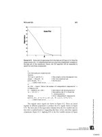
The inverse relationship between time and
frequency is shown in Figure 7.2, which was obtained by applying Eqs. (7–10)
to the Mexican hat wavelet. (The code for this is given in Example 7.2.) The
Mexican hat wavelet is given by the equation:
ψ(t) = (1 − 2t
2
)e
−t
2
(11)

TLFeBOOK
182 Chapter 7
F
IGURE
7.2 Time–frequency boundaries of the Mexican hat wavelet for various
values of a. The area of each of these boxes is constant (Eq. (12)). The code
that generates this figure is based on Eqs. (7–10) and is given in Example 7.2.
The frequency range, or bandwidth, would be the range of the mother
Wavelet divided by a: ∆ω
ψ
(a) =∆ω
ψ
/*a*. If we multiply the frequency range
by the time range, the a’s cancel and we are left with a constant that is the
product of the constants produced by Eq. (7) and (9):
∆ω
ψ
(a)∆t
ψ
(a) =∆ω
ψ
∆t
ψ
= constant
ψ
(12)
Eq. (12) shows that the product of the ranges is invariant to dilation* and
that the ranges are inversely related; increasing the frequency range, ∆ω
ψ
(a),

decreases the time range, ∆t
ψ
(a). These ranges correlate to the time and fre-
quency resolution of the CWT. Just as in the short-term Fourier transform, there
is a time–frequency trade-off (recall Eq. (3) in Chapter 6): decreasing the wave-
let time range (by decreasing a) provides a more accurate assessment of time
characteristics (i.e., the ability to separate out close events in time) at the ex-
pense of frequency resolution, and vice versa.
*Translations (changes in the variable b), do alter either the time or frequency resolution; hence,
both time and frequency resolution, as well as their product, are independent of the value of b.
TLFeBOOK
Wavelet Analysis 183
Since the time and frequency resolutions are inversely related, the CWT
will provide better frequency resolution when a is large and the length of the
wavelet (and its effective time window) is long. Conversely, when a is small,
the wavelet is short and the time resolution is maximum, but the wavelet only
responds to high frequency components. Since a is variable, there is a built-in
trade-off between time and frequency resolution, which is key to the CWT and
makes it well suited to analyzing signals with rapidly varying high frequency
components superimposed on slowly varying low frequency components.
MATLAB Implementation
A number of software packages exist in MATLAB for computing the continu-
ous wavelet transform, including MATLAB’s Wavelet Toolbox and Wavelab
which is available free over the Internet: (www.stat.stanford.edu/ϳwavelab/).
However, it is not difficult to implement Eq. (4) directly, as illustrated in the
example below.
Example 7.1 Write a program to construct the CWT of a signal consist-
ing of two sequential sine waves of 10 and 40 Hz. (i.e. the signal shown in
Figure 6.1). Plot the wavelet coefficients as a function of a and b. Use the
Morlet wavelet.

The signal waveform is constructed as in Example 6.1. A time vector,
ti
,
is generated that will be used to produce the positive half of the wavelet. This
vector is initially scaled so that the mother wavelet (a = 1) will be ± 10 sec
long. With each iteration, the value of a is adjusted (128 different values are
used in this program) and the wavelet time vector is it then scaled to produce
the appropriate wavelet family member. During each iteration, the positive half
of the Morlet wavelet is constructed using the defining equation (Eq. (5)), and
the negative half is generated from the positive half by concatenating a time
reversed (flipped) version with the positive side. The wavelet coefficients at a
given value of a are obtained by convolution of the scaled wavelet with the
signal. Since convolution in MATLAB produces extra points, these are removed
symmetrically (see Chapter 2), and the coefficients are plotted three-dimension-
ally against the values of a and b. The resulting plot, Figure 7.3, reflects the
time–frequency characteristics of the signal which are quantitatively similar to
those produced by the STFT and shown in Figure 6.2.
% Example 7.1 and Figure 7.3
% Generate 2 sinusoids that change frequency in a step-like
% manner
% Apply the continuous wavelet transform and plot results
%
clear all; close all;
% Set up constants
TLFeBOOK
184 Chapter 7
F
IGURE
7.3 Wavelet coefficients obtained by applying the CWT to a waveform
consisting of two sequential sine waves of 10 and 40 Hz, as shown in Figure 6.1.

The Morlet wavelet was used.
fs = 500 % Sample frequency
N = 1024; % Signal length
N1 = 512; % Wavelet number of points
f1 = 10; % First frequency in Hz
f2 = 40; % Second frequency in Hz
resol_level = 128; % Number of values of a
decr_a = .5; % Decrement for a
a_init = 4; % Initial a
wo = pi * sqrt(2/log2(2)); % Wavelet frequency scale
% factor
%
% Generate the two sine waves. Same as in Example 6.1
tn = (1:N/4)/fs; % Time vector to create
% sinusoids
b = (1:N)/fs; % Time vector for plotting
x = [zeros(N/4,1); sin(2*pi *f1*tn)’; sin(2*pi*f2*tn)’;
zeros(N/4,1)];
ti = ((1:N1/2)/fs)*10; % Time vector to construct
% ± 10 sec. of wavelet
TLFeBOOK
Wavelet Analysis 185
% Calculate continuous Wavelet transform
% Morlet wavelet, Eq. (5)
for i = 1:resol_level
a(i) = a_init/(1؉i*decr_a); % Set scale
t = abs(ti/a(i)); % Scale vector for wavelet
mor = (exp(-t.v2).* cos(wo*t))/ sqrt(a(i));
Wavelet = [fliplr(mor) mor]; % Make symmetrical about
% zero

ip = conv(x,Wavelet); % Convolve wavelet and
% signal
ex = fix((length(ip)-N)/2); % Calculate extra points /2
CW_Trans(:,i) =ip(ex؉1:N؉ex,1); % Remove extra points
% symmetrically
end
%
% Plot in 3 dimensions
d = fliplr(CW_Trans);
mesh(a,b,CW_Trans);
***** labels and view angle *****
In this example, a was modified by division with a linearly increasing
value. Often, wavelet scale is modified based on octaves or fractions of octaves.
A determination of the time–frequency boundaries of a wavelet though
MATLAB implementation of Eqs. (7–10) is provided in the next example.
Example 7.2 Find the time–frequency boundaries of the Mexican hat
wavelet.
For each of 4 values of a, the scaled wavelet is constructed using an
approach similar to that found in Example 7.1. The magnitude squared of the
frequency response is calculated using the FFT. The center time, t
0
, and center
frequency, w
0
, are constructed by direct application of Eqs. (8) and (10). Note
that since the wavelet is constructed symmetrically about t = 0, the center time,
t
0
, will always be zero, and an appropriate offset time, t
1

, is added during plot-
ting. The time and frequency boundaries are calculated using Eqs. (7) and (9),
and the resulting boundaries as are plotted as a rectangle about the appropriate
time and frequency centers.
% Example 7.2 and Figure 7.2
% Plot of wavelet boundaries for various values of ’a’
% Determines the time and scale range of the Mexican wavelet.
% Uses the equations for center time and frequency and for time
% and frequency spread given in Eqs. (7–10)
%
TLFeBOOK
186 Chapter 7
clear all; close all;
N = 1000; % Data length
fs = 1000; % Assumed sample frequency
wo1 = pi * sqrt(2/log2(2)); % Const. for wavelet time
% scale
a = [.5 1.0 2.0 3.0]; % Values of a
xi = ((1:N/2)/fs)*10; % Show ± 10 sec of the wavelet
t = (1:N)/fs; % Time scale
omaga = (1:N/2) * fs/N; % Frequency scale
%
for i = 1:length(a)
t1 = xi./a(i); % Make time vector for
% wavelet
mex = exp(-t1.v2).* (1–2*t1.v2);% Generate Mexican hat
% wavelet
w = [fliplr(mex) mex]; % Make symmetrical about zero
wsq = abs(w).v2 % Square wavelet;
W = fft(w); % Get frequency representa-

Wsq = abs(W(1:N/2)).v2; % tion and square. Use only
% fs /2 range
t0 = sum(t.* wsq)/sum(wsq); % Calculate center time
d_t = sqrt(sum((t—to).v2 .*wsq)/sum(wsq));
% Calculate time spread
w0 = sum(omaga.*Wsq)/sum(Wsq); % Calculate center frequency
d_w0 = sqrt(sum((omaga—w0).v2 .* Wsq)/sum(Wsq));
t1 = t0*a(i); % Adjust time position to
% compensate for symmetri-
% cal waveform
hold on;
% Plot boundaries
plot([t1-d_t t1-d_t],[w0-d_w0 w0؉d_w0],’k’);
plot([t1؉d_t t1؉d_t],[w0-d_w0 w0؉d_w0],’k’);
plot([t1-d_t t1؉d_t],[w0-d_w0 w0-d_w0],’k’);
plot([t1-d_t t1؉d_t],[w0؉d_w0 w0؉d_w0],’k’);
end
% ***** lables*****
THE DISCRETE WAVELET TRANSFORM
The CWT has one serious problem: it is highly redundant.* The CWT provides
an oversampling of the original waveform: many more coefficients are gener-
ated than are actually needed to uniquely specify the signal. This redundancy is
*In its continuous form, it is actually infinitely redundant!
TLFeBOOK
Wavelet Analysis 187
usually not a problem in analysis applications such as described above, but will
be costly if the application calls for recovery of the original signal. For recovery,
all of the coefficients will be required and the computational effort could be
excessive. In applications that require bilateral transformations, we would prefer
a transform that produces the minimum number of coefficients required to re-

cover accurately the original signal. The discrete wavelet transform (DWT)
achieves this parsimony by restricting the variation in translation and scale,
usually to powers of 2. When the scale is changed in powers of 2, the discrete
wavelet transform is sometimes termed the dyadic wavelet transform which,
unfortunately, carries the same abbreviation (DWT). The DWT may still require
redundancy to produce a bilateral transform unless the wavelet is carefully cho-
sen such that it leads to an orthogonal family (i.e., a orthogonal basis). In this
case, the DWT will produce a nonredundant, bilateral transform.
The basic analytical expressions for the DWT will be presented here; how-
ever, the transform is easier to understand, and easier to implement using filter
banks, as described in the next section. The theoretical link between filter banks
and the equations will be presented just before the MATLAB Implementation
section. The DWT is often introduced in terms of its recovery transform:
x(t) =
∑
∞
k=−∞
∑
∞
R =−∞
d(k,R)2
−k/2
ψ(2
−k
t − R) (13)
Here k is related to a as: a = 2
k
; b is related to R as b = 2
k
R; and d(k,R)is

a sampling of W(a,b) at discrete points k and R.
In the DWT, a new concept is introduced termed the scaling function,a
function that facilitates computation of the DWT. To implement the DWT effi-
ciently, the finest resolution is computed first. The computation then proceeds
to coarser resolutions, but rather than start over on the original waveform, the
computation uses a smoothed version of the fine resolution waveform. This
smoothed version is obtained with the help of the scaling function. In fact, the
scaling function is sometimes referred to as the smoothing function. The defini-
tion of the scaling function uses a dilation or a two-scale difference equation:
φ(t) =
∑
∞
n=−∞
√
2c(n)φ(2t − n) (14)
where c(n) is a series of scalars that defines the specific scaling function. This
equation involves two time scales (t and 2t) and can be quite difficult to solve.
In the DWT, the wavelet itself can be defined from the scaling function:
ψ(t) =
∑
∞
n=−∞
√
2d(n)φ(2t − n) (15)
TLFeBOOK
188 Chapter 7
where d(n) is a series of scalars that are related to the waveform x(t) (Eq. (13))
and that define the discrete wavelet in terms of the scaling function. While the
DWT can be implemented using the above equations, it is usually implemented
using filter bank techniques.

Filter Banks
For most signal and image processing applications, DWT-based analysis is best
described in terms of filter banks. The use of a group of filters to divide up a
signal into various spectral components is termed subband coding. The most
basic implementation of the DWT uses only two filters as in the filter bank
shown in Figure 7.4.
The waveform under analysis is divided into two components, y
lp
(n) and
y
hp
(n), by the digital filters H
0
(ω) and H
1
(ω). The spectral characteristics of the
two filters must be carefully chosen with H
0
(ω) having a lowpass spectral char-
acteristic and H
1
(ω) a highpass spectral characteristic. The highpass filter is
analogous to the application of the wavelet to the original signal, while the
lowpass filter is analogous to the application of the scaling or smoothing func-
tion. If the filters are invertible filters, then it is possible, at least in theory, to
construct complementary filters (filters that have a spectrum the inverse of H
0
(ω)
or H
1

(ω)) that will recover the original waveform from either of the subband
signals, y
lp
(n)ory
hp
(n). The original signal can often be recovered even if the
filters are not invertible, but both subband signals will need to be used. Signal
recovery is illustrated in Figure 7.5 where a second pair of filters, G
0
(ω) and
G
1
(ω), operate on the high and lowpass subband signals and their sum is used
F
IGURE
7.4 Simple filter bank consisting of only two filters applied to the same
waveform. The filters have lowpass and highpass spectral characteristics. Filter
outputs consist of a lowpass subband, y
lp
(n), and a highpass subband, y
hp
(n).
TLFeBOOK
Wavelet Analysis 189
F
IGURE
7.5 A typical wavelet application using filter banks containing only two
filters. The input waveform is first decomposed into subbands using the analysis
filter bank. Some process is applied to the filtered signals before reconstruction.
Reconstruction is performed by the synthesis filter bank.

to reconstruct a close approximation of the original signal, x’(t). The Filter Bank
that decomposes the original signal is usually termed the analysis filters while
the filter bank that reconstructs the signal is termed the syntheses filters. FIR
filters are used throughout because they are inherently stable and easier to im-
plement.
Filtering the original signal, x(n), only to recover it with inverse filters
would be a pointless operation, although this process may have some instructive
value as shown in Example 7.3. In some analysis applications only the subband
signals are of interest and reconstruction is not needed, but in many wavelet
applications, some operation is performed on the subband signals, y
lp
(n) and
y
hp
(n), before reconstruction of the output signal (see Figure 7.5). In such cases,
the output will no longer be exactly the same as the input. If the output is
essentially the same, as occurs in some data compression applications, the pro-
cess is termed lossless, otherwise it is a lossy operation.
There is one major concern with the general approach schematized in
Figure 7.5: it requires the generation of, and operation on, twice as many points
as are in the original waveform x(n). This problem will only get worse if more
filters are added to the filter bank. Clearly there must be redundant information
contained in signals y
lp
(n) and y
hp
(n), since they are both required to represent
x(n), but with twice the number of points. If the analysis filters are correctly
chosen, then it is possible to reduce the length of y
lp

(n) and y
hp
(n) by one half
and still be able to recover the original waveform. To reduce the signal samples
by one half and still represent the same overall time period, we need to eliminate
every other point, say every odd point. This operation is known as downsam-
pling and is illustrated schematically by the symbol ↓ 2. The downsampled ver-
sion of y(n) would then include only the samples with even indices [y(2), y(4),
y(6), ]ofthefiltered signal.
TLFeBOOK
190 Chapter 7
If downsampling is used, then there must be some method for recovering
the missing data samples (those with odd indices) in order to reconstruct the
original signal. An operation termed upsampling (indicated by the symbol ↑ 2)
accomplishes this operation by replacing the missing points with zeros. The
recovered signal (x’(n) in Figure 7.5) will not contain zeros for these data sam-
ples as the synthesis filters, G
0
(ω)orG
1
(ω), ‘fill in the blanks.’ Figure 7.6
shows a wavelet application that uses three filter banks and includes the down-
sampling and upsampling operations. Downsampled amplitudes are sometimes
scaled by
√
2, a normalization that can simplify the filter calculations when
matrix methods are used.
Designing the filters in a wavelet filter bank can be quite challenging
because the filters must meet a number of criteria. A prime concern is the ability
to recover the original signal after passing through the analysis and synthesis

filter banks. Accurate recovery is complicated by the downsampling process.
Note that downsampling, removing every other point, is equivalent to sampling
the original signal at half the sampling frequency. For some signals, this would
lead to aliasing, since the highest frequency component in the signal may no
F
IGURE
7.6 A typical wavelet application using three filters. The downsampling
( ↓ 2) and upsampling ( ↑ 2) processes are shown. As in Figure 7.5, some pro-
cess would be applied to the filtered signals, y
lp
(n) and y
hp
(n), before reconstruc-
tion.
TLFeBOOK
Wavelet Analysis 191
longer be twice the now reduced sampling frequency. Appropriately chosen fil-
ter banks can essentially cancel potential aliasing. If the filter bank contains
only two filter types (highpass and lowpass filters) as in Figure 7.5, the criterion
for aliasing cancellation is (Strang and Nguyen, 1997):
G
0
(z)H
0
(−z) + G
1
(z)H
1
(−z) = 0 (16)
where H

0
(z) is the transfer function of the analysis lowpass filter, H
1
(z)isthe
transfer function of the analysis highpass filter, G
0
(z) is the transfer function of
the synthesis lowpass filter, and G
1
(z) is the transfer function of the synthesis
highpass filter.
The requirement to be able to recover the original waveform from the
subband waveforms places another important requirement on the filters which
is satisfied when:
G
0
(z)H
0
(z) + G
1
(z)H
1
(z) = 2z
−N
(17)
where the transfer functions are the same as those in Eq. (16). N is the number
of filter coefficients (i.e., the filter order); hence z
-N
is just the delay of the filter.
In many analyses, it is desirable to have subband signals that are orthogo-

nal, placing added constraints on the filters. Fortunately, a number of filters
have been developed that have most of the desirable properties.* The examples
below use filters developed by Daubechies, and named after her. This is a family
of popular wavelet filters having 4 or more coefficients. The coefficients of the
lowpass filter, h
0
(n), for the 4-coefficient Daubechies filter are given as:
h(n) =
[(1 +
√
3), (3 +
√
3), (3 −
√
3), (1 −
√
3)]
8
(18)
Other, higher order filters in this family are given in the MATLAB routine
daub
found in the routines associated with this chapter. It can be shown that
orthogonal filters with more than two coefficients must have asymmetrical coef-
ficients.† Unfortunately this precludes these filters from having linear phase
characteristics; however, this is a compromise that is usually acceptable. More
complicated biorthogonal filters (Strang and Nguyen, 1997) are required to pro-
duce minimum phase and orthogonality.
In order for the highpass filter output to be orthogonal to that of the low-
pass output, the highpass filter frequency characteristics must have a specific
relationship to those of the lowpass filter:

*Although no filter yet exists that has all of the desirable properties.
†The two-coefficient, orthogonal filter is: h(n) = [
1
⁄
2
;
1
⁄
2
], and is known as the Haar filter. Essentially
a two -point moving average, this filter does not have very strong filter characteristics. See Problem 3 .
TLFeBOOK
192 Chapter 7
H
1
(z) =−z
−N
H
0
(−z
−1
)(19)
The criterion represented by Eq. (19) can be implemented by applying the
alternating flip algorithm to the coefficients of h
0
(n):
h
1
(n) = [h
0

(N), −h
0
(N − 1), h
0
(N − 2), −h
0
(N − 3), ] (20)
where N is the number of coefficients in h
0
(n). Implementation of this alternat-
ing flip algorithm is found in the
analyze
program of Example 7.3.
Once the analyze filters have been chosen, the synthesis filters used for
reconstruction are fairly constrained by Eqs. (14) and (15). The conditions of
Eq. (17) can be met by making G
0
(z) = H
1
(- z) and G
1
(z) = -H
0
(-z). Hence the
synthesis filter transfer functions are related to the analysis transfer functions
by the Eqs. (21) and (22):
G
0
(z) = H
1

(z) = z
−N
H
0
(z
−1
)(21)
G
1
(z) =−H
0
(−z) = z
−N
H
1
(z
−1
)(22)
where the second equality comes from the relationship expressed in Eq. (19).
The operations of Eqs. (21) and (22) can be implemented several different ways,
but the easiest way in MATLAB is to use the second equalities in Eqs. (21) and
(22), which can be implemented using the order flip algorithm:
g
0
(n) = [h
0
(N), h
0
(N − 1), h
0

(N − 2), ] (23)
g
1
(n) = [h
1
(N), h
1
(N − 1), h
1
(N − 2), ] (24)
where, again, N is the number of filter coefficients. (It is assumed that all filters
have the same order; i.e., they have the same number of coefficients.)
An example of constructing the syntheses filter coefficients from only the
analysis filter lowpass filter coefficients, h
0
(n), is shown in Example 7.3. First
the alternating flip algorithm is used to get the highpass analysis filter coeffi-
cients, h
1
(n), then the order flip algorithm is applied as in Eqs. (23) and (24) to
produce both the synthesis filter coefficients, g
0
(n) and g
1
(n).
Note that if the filters shown in Figure 7.6 are causal, each would produce
a delay that is dependent on the nu mber of filter coefficients. Such delays are
expected and natural , and may have to be taken into account in the reconstru ction
process. However, when the data are stored in the computer it is possible to
implement FIR filters without a delay. An example of the use of periodic convolu-

tion to eliminate the delay is shown in Example 7.4 ( see also Chapter 2).
The Relationship Between Analytical Expressions
and Filter Banks
The filter bank approach and the discrete wavelet transform represented by Eqs.
(14) and (15) were actually developed separately, but have become linked both
TLFeBOOK
Wavelet Analysis 193
theoretically and practically. It is possible, at least in theory, to go between
the two approaches to develop the wavelet and scaling function from the filter
coefficients and vice versa. In fact, the coefficients c(n) and d(n) in Eqs. (14)
and (15) are simply scaled versions of the filter coefficients:
c(n) =
√
2 h
0
(n); d(n) =
√
2 h
1
(n) (25)
With the substitution of c(n) in Eq. (14), the equation for the scaling
function (the dilation equation) becomes:
φ(t) =
∑
∞
n=−∞
2 h
0
(n)φ(2t − n) (26)
Since this is an equation with two time scales (t and 2t), it is not easy to

solve, but a number of approximation approaches have been worked out (Strang
and Nguyen, 1997, pp. 186–204). A number of techniques exist for solving for
φ(t) in Eq. (26) given the filter coefficients, h
1
(n). Perhaps the most straightfor-
ward method of solving for φ in Eq. (26) is to use the frequency domain repre-
sentation. Taking the Fourier transform of both sides of Eq. (26) gives:
Φ(ω) = H
0
ͩ
ω
2
ͪ
Φ
ͩ
ω
2
ͪ
(27)
Note that 2t goes to ω/2 in the frequency domain. The second term in Eq.
(27) can be broken down into H
0
(ω/4) Φ(ω/4), so it is possible to rewrite the
equation as shown below.
Φ(ω) = H
0
ͩ
ω
2
ͪͫ

H
0
ͩ
ω
4
ͪ
Φ
ͩ
ω
4
ͪ
ͬ
(28)
= H
0
ͩ
ω
2
ͪ
H
0
ͩ
ω
4
ͪ
H
0
ͩ
ω
8

ͪ
H
0
ͩ
ω
2
N
ͪ
Φ
ͩ
ω
2
N
ͪ
(29)
In the limit as N →∞, Eq. (29) becomes:
Φ(ω) =
J
∞
j=1
H
0
ͩ
ω
2
j
ͪ
(30)
The relationship between φ(t) and the lowpass filter coefficients can now
be obtained by taking the inverse Fourier transform of Eq. (30). Once the scaling

function is determined, the wavelet function can be obtained directly from Eq.
(16) with 2h
1
(n) substituted for d(n):
ψ(t) =
∑
∞
n=−∞
2 h
1
(n)φ(2t − n) (31)
TLFeBOOK
194 Chapter 7
Eq. (30) also demonstrates another constraint on the lowpass filter coeffi-
cients, h
0
(n), not mentioned above. In order for the infinite product to converge
(or any infinite product for that matter), H
0
(ω/2
j
) must approach 1 as j →∞.
This implies that H
0
(0) = 1, a criterion that is easy to meet with a lowpass filter.
While Eq. (31) provides an explicit formula for determining the scaling function
from the filter coefficients, an analytical solution is challenging except for very
simple filters such as the two-coefficient Haar filter. Solving this equation nu-
merically also has problems due to the short data length (H
0

(ω) would be only
4 points for a 4-element filter). Nonetheless, the equation provides a theoretical
link between the filter bank and DWT methodologies.
These issues described above, along with some applications of wavelet
analysis, are presented in the next section on implementation.
MATLAB Implementation
The construction of a filter bank in MATLAB can be achieved using either
routines from the Signal Processing Toolbox,
filter
or
filtfilt
, or simply
convolution. All examples below use convolution. Convolution does not con-
serve the length of the original waveform: the MATLAB
conv
produces an
output with a length equal to the data length plus the filter length minus one.
Thus with a 4-element filter the output of the convolution process would be 3
samples longer than the input. In this example, the extra points are removed by
simple truncation. In Example 7.4, circular or periodic convolution is used to
eliminate phase shift. Removal of the extraneous points is followed by down-
sampling, although these two operations could be done in a single step, as shown
in Example 7.4.
The main program shown below makes use of 3 important subfunctions.
The routine
daub
is available on the disk and supplies the coefficients of a
Daubechies filter using a simple list of coefficients. In this example, a 6-element
filter is used, but the routine can also generate coefficients of 4-, 8-, and 10-
element Daubechies filters.

The waveform is made up of 4 sine waves of different frequencies with
added noise. This waveform is decomposed into 4 subbands using the routine
analysis
. The subband signals are plotted and then used to reconstruct the
original signal in the routine
synthesize
. Since no operation is performed on
the subband signals, the reconstructed signal should match the original except
for a phase shift.
Example 7.3 Construct an analysis filter bank containing
L
decomposi-
tions; that is, a lowpass filter and
L
highpass filters. Decompose a signal consist-
ing of 4 sinusoids in noise and the recover this signal using an
L
-level syntheses
filter bank.
TLFeBOOK
Wavelet Analysis 195
% Example 7.3 and Figures 7.7 and 7.8
% Dyadic wavelet transform example
% Construct a waveform of 4 sinusoids plus noise
% Decompose the waveform in 4 levels, plot each level, then
% reconstruct
% Use a Daubechies 6-element filter
%
clear all; close all;
%

fs = 1000; % Sample frequency
N = 1024; % Number of points in
% waveform
freqsin = [.63 1.1 2.7 5.6]; % Sinusoid frequencies
% for mix
ampl = [1.2 1 1.2 .75 ]; % Amplitude of sinusoid
h0 = daub(6); % Get filter coeffi-
% cients: Daubechies 6
F
IGURE
7.7 Input (middle) waveform to the four-level analysis and synthesis filter
banks used in Example 7.3. The lower waveform is the reconstructed output from
the synthesis filters. Note the phase shift due to the causal filters. The upper
waveform is the original signal before the noise was added.
TLFeBOOK
196 Chapter 7
F
IGURE
7.8 Signals generated by the analysis filter bank used in Example 7.3
with the top-most plot showing the outputs of the first set of filters with the finest
resolution, the next from the top showing the outputs of the second set of set of
filters, etc. Only the lowest (i.e., smoothest) lowpass subband signal is included
in the output of the filter bank; the rest are used only in the determination of
highpass subbands. The lowest plots show the frequency characteristics of the
high- and lowpass filters.
%
[x t] = signal(freqsin,ampl,N); % Construct signal
x1 = x ؉ (.25 * randn(1,N)); % Add noise
an = analyze(x1,h0,4); % Decompose signal,
% analytic filter bank

sy = synthesize(an,h0,4); % Reconstruct original
% signal
figure(fig1);
plot(t,x,’k’,t,x1–4,’k’,t,sy-8,’k’);% Plot signals separated
TLFeBOOK
Wavelet Analysis 197
This program uses the function
signal
to generate the mixtures of sinu-
soids. This routine is similar to
sig_noise
except that it generates only mix-
tures of sine waves without the noise. The first argument specifies the frequency
of the sines and the third argument specifies the number of points in the wave-
form just as in
sig_noise
. The second argument specifies the amplitudes of
the sinusoids, not the SNR as in
sig_noise
.
The
analysis
function shown below implements the analysis filter bank.
This routine first generates the highpass filter coefficients,
h1
, from the lowpass
filter coefficients,
h
, using the alternating flip algorithm of Eq. (20). These FIR
filters are then applied using standard convolution. All of the various subband

signals required for reconstruction are placed in a single output array,
an
. The
length of
an
is the same as the length of the input,
N
= 1024 in this example.
The only lowpass signal needed for reconstruction is the smoothest lowpass
subband (i.e., final lowpass signal in the lowpass chain), and this signal is placed
in the first data segment of
an
taking up the first
N
/16 data points. This signal
is followed by the last stage highpass subband which is of equal length. The
next
N
/8 data points contain the second to last highpass subband followed, in
turn, by the other subband signals up to the final, highest resolution highpass
subband which takes up all of the second half of
an
. The remainder of the
analyze
routine calculates and plots the high- and lowpass filter frequency
characteristics.
% Function to calculate analyze filter bank
%an = analyze(x,h,L)
% where
%x= input waveform in column form which must be longer than

%2vL ؉ L and power of two.
%h0= filter coefficients (lowpass)
%L= decomposition level (number of highpass filter in bank)
%
function an = analyze(x,h0,L)
lf = length(h0); % Filter length
lx = length(x); % Data length
an = x; % Initialize output
% Calculate High pass coefficients from low pass coefficients
for i = 0:(lf-1)
h1(i؉1) = (-1)vi * h0(lf-i); % Alternating flip, Eq. (20)
end
%
% Calculate filter outputs for all levels
for i = 1:L
a_ext = an;
TLFeBOOK
198 Chapter 7
lpf = conv(a_ext,h0); % Lowpass FIR filter
hpf = conv(a_ext,h1); % Highpass FIR filter
lpf = lpf(1:lx); % Remove extra points
hpf = hpf(1:lx);
lpfd = lpf(1:2:end); % Downsample
hpfd = hpf(1:2:end);
an(1:lx) = [lpfd hpfd]; % Low pass output at beginning
% of array, but now occupies
% only half the data
% points as last pass
lx = lx/2;
subplot(L؉1,2,2*i-1); % Plot both filter outputs

plot(an(1:lx)); % Lowpass output
if i == 1
title(’Low Pass Outputs’); % Titles
end
subplot(L؉1,2,2*i);
plot(an(lx؉1:2*lx)); % Highpass output
if i == 1
title(’High Pass Outputs’)
end
end
%
HPF = abs(fft(h1,256)); % Calculate and plot filter
LPF = abs(fft(h0,256)); % transfer fun of high- and
% lowpass filters
freq = (1:128)* 1000/256; % Assume fs = 1000 Hz
subplot(L؉1,2,2*i؉1);
plot(freq, LPF(1:128)); % Plot from 0 to fs/2 Hz
text(1,1.7,’Low Pass Filter’);
xlabel(’Frequency (Hz.)’)’
subplot(L؉1,2,2*i؉2);
plot(freq, HPF(1:128));
text(1,1.7,’High Pass Filter’);
xlabel(’Frequency (Hz.)’)’
The original data are reconstructed from the analyze filter bank signals in
the program
synthesize
. This program first constructs the synthesis lowpass
filter,
g0
, using order flip applied to the analysis lowpass filter coefficients

(Eq. (23)). The analysis highpass filter is constructed using the alternating flip
algorithm (Eq. (20)). These coefficients are then used to construct the synthesis
highpass filter coefficients through order flip (Eq. (24)). The synthesis filter
loop begins with the course signals first, those in the initial data segments of
a
with the shortest segment lengths. The lowpass and highpass signals are upsam-
pled, then filtered using convolution, the additional points removed, and the
signals added together. This loop is structured so that on the next pass the
TLFeBOOK
Wavelet Analysis 199
recently combined segment is itself combined with the next higher resolution
highpass signal. This iterative process continues until all of the highpass signals
are included in the sum.
% Function to calculate synthesize filter bank
%y = synthesize(a,h0,L)
% where
%a= analyze filter bank outputs (produced by analyze)
%h= filter coefficients (lowpass)
%L= decomposition level (number of highpass filters in bank)
%
function y = synthesize(a,h0,L)
lf = length(h0); % Filter length
lx = length(a); % Data length
lseg = lx/(2vL); % Length of first low- and
% highpass segments
y = a; % Initialize output
g0 = h0(lf:-1:1); % Lowpass coefficients using
% order flip, Eq. (23)
% Calculate High pass coefficients, h1(n), from lowpass
% coefficients use Alternating flip Eq. (20)

for i = 0:(lf-1)
h1(i؉1) = (-1)vi * h0(lf-i);
end
g1 = h1(lf:-1:1); % Highpass filter coeffi-
% cients using order
% flip, Eq. (24 )
% Calculate filter outputs for all levels
for i = 1:L
lpx = y(1:lseg); % Get lowpass segment
hpx = y(lseg؉1:2*lseg); % Get highpass outputs
up_lpx = zeros(1,2*lseg); % Initialize for upsampling
up_lpx(1:2:2*lseg) = lpx; % Upsample lowpass (every
% odd point)
up_hpx = zeros(1,2*lseg); % Repeat for highpass
up_hpx(1:2:2*lseg) = hpx;
syn = conv(up_lpx,g0) ؉ conv(up_hpx,g1); % Filter and
% combine
y(1:2*lseg) = syn(1:(2*lseg) ); % Remove extra points from
% end
lseg = lseg * 2; % Double segment lengths for
% next pass
end
The subband signals are shown in Figure 7.8. Also shown are the fre-
quency characteristics of the Daubechies high- and lowpass filters. The input
TLFeBOOK
200 Chapter 7
and reconstructed output waveforms are shown in Figure 7.7. The original signal
before the noise was added is included. Note that the reconstructed waveform
closely matches the input except for the phase lag introduced by the filters. As
shown in the next example, this phase lag can be eliminated by using circular

or periodic convolution, but this will also introduce some artifact.
Denoising
Example 7.3 was not particularly practical since the reconstructed signal was
the same as the original, except for the phase shift. A more useful application
of wavelets is shown in Example 7.4, where some processing is done on the
subband signals before reconstruction—in this example, nonlinear filtering. The
basic assumption in this application is that the noise is coded into small fluctua-
tions in the higher resolution (i.e., more detailed) highpass subbands. This noise
can be selecti ve ly reduced by eliminating the smaller sample values in the higher
resolut io n hi gh pas s subbands. In thi s e xample, the two highe st resolution hig hp ass
subband s are examined and data points below so me thresh ol d are zeroed out. The
thresho ld is set to be equal to the variance of the highpa ss subbands .
Example 7.4 Decompose the signal in Example 7.3 using a 4-level filter
bank. In this example, use periodic convolution in the analysis and synthesis
filters and a 4-element Daubechies filter. Examine the two highest resolution
highpass subbands. These subbands will reside in the last N/4 to N samples. Set
all values in these segments that are below a given threshold value to zero. Use
the net variance of the subbands as the threshold.
% Example 7.4 and Figure 7.9
% Application of DWT to nonlinear filtering
% Construct the waveform in Example 7.3.
% Decompose the waveform in 4 levels, plot each level, then
% reconstruct.
% Use Daubechies 4-element filter and periodic convolution.
% Evaluate the two highest resolution highpass subbands and
% zero out those samples below some threshold value.
%
close all; clear all;
fs = 1000; % Sample frequency
N = 1024; % Number of points in

% waveform
%
freqsin = [.63 1.1 2.7 5.6]; % Sinusoid frequencies
ampl = [1.2 1 1.2 .75 ]; % Amplitude of sinusoids
[x t] = signal(freqsin,ampl,N); % Construct signal
x = x ؉ (.25 * randn(1,N)); % and add noise
h0 = daub(4);
figure(fig1);
TLFeBOOK
Wavelet Analysis 201
F
IGURE
7.9 Application of the dyadic wavelet transform to nonlinear filtering.
After subband decomposition using an analysis filter bank, a threshold process is
applied to the two highest resolution highpass subbands before reconstruction
using a synthesis filter bank. Periodic convolution was used so that there is no
phase shift between the input and output signals.
an = analyze1(x,h0,4); % Decompose signal, analytic
% filter bank of level 4
% Set the threshold times to equal the variance of the two higher
% resolution highpass subbands.
threshold = var(an(N/4:N));
for i = (N/4:N) % Examine the two highest
% resolution highpass
% subbands
if an(i) < threshold
an(i) = 0;
end
end
sy = synthesize1(an,h0,4); % Reconstruct original

% signal
figure(fig2);
plot(t,x,’k’,t,sy-5,’k’); % Plot signals
axis([ 2 1.2-8 4]); xlabel(’Time(sec)’)
TLFeBOOK
202 Chapter 7
The routines for the analysis and synthesis filter banks differ slightly from
those used in Example 7.3 in that they use circular convolution. In the analysis
filter bank routine (
analysis1
), the data are first extended using the periodic
or wraparound approach: the initial points are added to the end of the original
data sequence (see Figure 2.10B). This extension is the same length as the
filter. After convolution, these added points and the extra points generated by
convolution are removed in a symmetrical fashion: a number of points equal to
the filter length are removed from the initial portion of the output and the re-
maining extra points are taken off the end. Only the code that is different from
that shown in Example 7.3 is shown below. In this code, symmetric elimination
of the additional points and downsampling are done in the same instruction.
function an = analyze1(x,h0,L)

for i = 1:L
a_ext = [an an(1:lf)]; % Extend data for “periodic
% convolution”
lpf = conv(a_ext,h0); % Lowpass FIR filter
hpf = conv(a_ext,h1); % Highpass FIR filter
lpfd = lpf(lf:2:lf؉lx-1); % Remove extra points. Shift to
hpfd = hpf(lf:2:lf؉lx-1); % obtain circular segment; then
% downsample
an(1:lx) = [lpfd hpfd]; % Lowpass output at beginning of

% array, but now occupies only
% half the data points as last
% pass
lx = lx/2;
The synthesis filter bank routine is modified in a similar fashion except
that the initial portion of the data is extended, also in wraparound fashion (by
adding the end points to the beginning). The extended segments are then upsam-
pled, convolved with the filters, and added together. The extra points are then
removed in the same manner used in the analysis routine. Again, only the modi-
fied code is shown below.
function y = synthesize1(an,h0,L)

for i = 1:L
lpx = y(1:lseg); % Get lowpass segment
hpx = y(lseg؉1:2*lseg); % Get highpass outputs
lpx = [lpx(lseg-lf/2؉1:lseg) lpx]; % Circular extension:
% lowpass comp.
hpx = [hpx(lseg-lf/2؉1:lseg) hpx]; % and highpass component
l_ext = length(lpx);
TLFeBOOK