Fluid Mechanics.McGraw-Hill Series in Mechanical Engineering CONSULTING EDITORSJack P. Holman, ppsx
Bạn đang xem bản rút gọn của tài liệu. Xem và tải ngay bản đầy đủ của tài liệu tại đây (12.38 MB, 1,023 trang )
Fluid Mechanics
McGraw-Hill Series in Mechanical Engineering
CONSULTING EDITORS
Jack P. Holman, Southern Methodist University
John Lloyd, Michigan State University
Anderson
Computational Fluid Dynamics: The Basics with Applications
Anderson
Modern Compressible Flow: With Historical Perspective
Arora
Introduction to Optimum Design
Borman and Ragland
Combustion Engineering
Burton
Introduction to Dynamic Systems Analysis
Culp
Principles of Energy Conversion
Dieter
Engineering Design: A Materials & Processing Approach
Doebelin
Engineering Experimentation: Planning, Execution, Reporting
Driels
Linear Control Systems Engineering
Edwards and McKee
Fundamentals of Mechanical Component Design
Gebhart
Heat Conduction and Mass Diffusion
Gibson
Principles of Composite Material Mechanics
Hamrock
Fundamentals of Fluid Film Lubrication
Heywood
Internal Combustion Engine Fundamentals
Kimbrell
Kinematics Analysis and Synthesis
Kreider and Rabl
Heating and Cooling of Buildings
Martin
Kinematics and Dynamics of Machines
Mattingly
Elements of Gas Turbine Propulsion
Modest
Radiative Heat Transfer
Norton
Design of Machinery
Oosthuizen and Carscallen
Compressible Fluid Flow
Oosthuizen and Naylor
Introduction to Convective Heat Transfer Analysis
Phelan
Fundamentals of Mechanical Design
Reddy
An Introduction to Finite Element Method
Rosenberg and Karnopp
Introduction to Physical Systems Dynamics
Schlichting
Boundary-Layer Theory
Shames
Mechanics of Fluids
Shigley
Kinematic Analysis of Mechanisms
Shigley and Mischke
Mechanical Engineering Design
Shigley and Uicker
Theory of Machines and Mechanisms
Hinze
Turbulence
Stiffler
Design with Microprocessors for Mechanical Engineers
Histand and Alciatore
Introduction to Mechatronics and Measurement Systems
Stoecker and Jones
Refrigeration and Air Conditioning
Holman
Experimental Methods for Engineers
Turns
An Introduction to Combustion: Concepts and Applications
Howell and Buckius
Fundamentals of Engineering Thermodynamics
Ullman
The Mechanical Design Process
Jaluria
Design and Optimization of Thermal Systems
Wark
Advanced Thermodynamics for Engineers
Juvinall
Engineering Considerations of Stress, Strain, and Strength
Wark and Richards
Thermodynamics
Kays and Crawford
Convective Heat and Mass Transfer
White
Viscous Fluid Flow
Kelly
Fundamentals of Mechanical Vibrations
Zeid
CAD/CAM Theory and Practice
Fluid Mechanics
Fourth Edition
Frank M. White
University of Rhode Island
Boston
Burr Ridge, IL Dubuque, IA Madison, WI New York San Francisco St. Louis
Bangkok Bogotá Caracas Lisbon London Madrid
Mexico City Milan New Delhi Seoul Singapore Sydney Taipei Toronto
About the Author
Frank M. White is Professor of Mechanical and Ocean Engineering at the University
of Rhode Island. He studied at Georgia Tech and M.I.T. In 1966 he helped found, at
URI, the first department of ocean engineering in the country. Known primarily as a
teacher and writer, he has received eight teaching awards and has written four textbooks on fluid mechanics and heat transfer.
During 1979–1990 he was editor-in-chief of the ASME Journal of Fluids Engineering and then served from 1991 to 1997 as chairman of the ASME Board of Editors and of the Publications Committee. He is a Fellow of ASME and in 1991 received
the ASME Fluids Engineering Award. He lives with his wife, Jeanne, in Narragansett,
Rhode Island.
v
To Jeanne
Preface
General Approach
The fourth edition of this textbook sees some additions and deletions but no philosophical change. The basic outline of eleven chapters and five appendices remains the
same. The triad of integral, differential, and experimental approaches is retained and
is approached in that order of presentation. The book is intended for an undergraduate
course in fluid mechanics, and there is plenty of material for a full year of instruction.
The author covers the first six chapters and part of Chapter 7 in the introductory semester. The more specialized and applied topics from Chapters 7 to 11 are then covered at our university in a second semester. The informal, student-oriented style is retained and, if it succeeds, has the flavor of an interactive lecture by the author.
Learning Tools
Approximately 30 percent of the problem exercises, and some fully worked examples,
have been changed or are new. The total number of problem exercises has increased
to more than 1500 in this fourth edition. The focus of the new problems is on practical and realistic fluids engineering experiences. Problems are grouped according to
topic, and some are labeled either with an asterisk (especially challenging) or a computer-disk icon (where computer solution is recommended). A number of new photographs and figures have been added, especially to illustrate new design applications
and new instruments.
Professor John Cimbala, of Pennsylvania State University, contributed many of the
new problems. He had the great idea of setting comprehensive problems at the end of
each chapter, covering a broad range of concepts, often from several different chapters. These comprehensive problems grow and recur throughout the book as new concepts arise. Six more open-ended design projects have been added, making 15 projects
in all. The projects allow the student to set sizes and parameters and achieve good design with more than one approach.
An entirely new addition is a set of 95 multiple-choice problems suitable for preparing for the Fundamentals of Engineering (FE) Examination. These FE problems come
at the end of Chapters 1 to 10. Meant as a realistic practice for the actual FE Exam,
they are engineering problems with five suggested answers, all of them plausible, but
only one of them correct.
xi
xii
Preface
New to this book, and to any fluid mechanics textbook, is a special appendix, Appendix E, Introduction to the Engineering Equation Solver (EES), which is keyed to
many examples and problems throughout the book. The author finds EES to be an extremely attractive tool for applied engineering problems. Not only does it solve arbitrarily complex systems of equations, written in any order or form, but also it has builtin property evaluations (density, viscosity, enthalpy, entropy, etc.), linear and nonlinear
regression, and easily formatted parameter studies and publication-quality plotting. The
author is indebted to Professors Sanford Klein and William Beckman, of the University of Wisconsin, for invaluable and continuous help in preparing this EES material.
The book is now available with or without an EES problems disk. The EES engine is
available to adopters of the text with the problems disk.
Another welcome addition, especially for students, is Answers to Selected Problems. Over 600 answers are provided, or about 43 percent of all the regular problem
assignments. Thus a compromise is struck between sometimes having a specific numerical goal and sometimes directly applying yourself and hoping for the best result.
Content Changes
There are revisions in every chapter. Chapter 1—which is purely introductory and
could be assigned as reading—has been toned down from earlier editions. For example, the discussion of the fluid acceleration vector has been moved entirely to Chapter 4. Four brief new sections have been added: (1) the uncertainty of engineering
data, (2) the use of EES, (3) the FE Examination, and (4) recommended problemsolving techniques.
Chapter 2 has an improved discussion of the stability of floating bodies, with a fully
derived formula for computing the metacentric height. Coverage is confined to static
fluids and rigid-body motions. An improved section on pressure measurement discusses
modern microsensors, such as the fused-quartz bourdon tube, micromachined silicon
capacitive and piezoelectric sensors, and tiny (2 mm long) silicon resonant-frequency
devices.
Chapter 3 tightens up the energy equation discussion and retains the plan that
Bernoulli’s equation comes last, after control-volume mass, linear momentum, angular momentum, and energy studies. Although some texts begin with an entire chapter
on the Bernoulli equation, this author tries to stress that it is a dangerously restricted
relation which is often misused by both students and graduate engineers.
In Chapter 4 a few inviscid and viscous flow examples have been added to the basic partial differential equations of fluid mechanics. More extensive discussion continues in Chapter 8.
Chapter 5 is more successful when one selects scaling variables before using the pi
theorem. Nevertheless, students still complain that the problems are too ambiguous and
lead to too many different parameter groups. Several problem assignments now contain a few hints about selecting the repeating variables to arrive at traditional pi groups.
In Chapter 6, the “alternate forms of the Moody chart” have been resurrected as
problem assignments. Meanwhile, the three basic pipe-flow problems—pressure drop,
flow rate, and pipe sizing—can easily be handled by the EES software, and examples
are given. Some newer flowmeter descriptions have been added for further enrichment.
Chapter 7 has added some new data on drag and resistance of various bodies, notably
biological systems which adapt to the flow of wind and water.
Preface
xiii
Chapter 8 picks up from the sample plane potential flows of Section 4.10 and plunges
right into inviscid-flow analysis, especially aerodynamics. The discussion of numerical methods, or computational fluid dynamics (CFD), both inviscid and viscous, steady
and unsteady, has been greatly expanded. Chapter 9, with its myriad complex algebraic
equations, illustrates the type of examples and problem assignments which can be
solved more easily using EES. A new section has been added about the suborbital X33 and VentureStar vehicles.
In the discussion of open-channel flow, Chapter 10, we have further attempted to
make the material more attractive to civil engineers by adding real-world comprehensive problems and design projects from the author’s experience with hydropower projects. More emphasis is placed on the use of friction factors rather than on the Manning roughness parameter. Chapter 11, on turbomachinery, has added new material on
compressors and the delivery of gases. Some additional fluid properties and formulas
have been included in the appendices, which are otherwise much the same.
Supplements
The all new Instructor’s Resource CD contains a PowerPoint presentation of key text
figures as well as additional helpful teaching tools. The list of films and videos, formerly App. C, is now omitted and relegated to the Instructor’s Resource CD.
The Solutions Manual provides complete and detailed solutions, including problem statements and artwork, to the end-of-chapter problems. It may be photocopied for
posting or preparing transparencies for the classroom.
EES Software
The Engineering Equation Solver (EES) was developed by Sandy Klein and Bill Beckman, both of the University of Wisconsin—Madison. A combination of equation-solving
capability and engineering property data makes EES an extremely powerful tool for your
students. EES (pronounced “ease”) enables students to solve problems, especially design
problems, and to ask “what if” questions. EES can do optimization, parametric analysis,
linear and nonlinear regression, and provide publication-quality plotting capability. Simple to master, this software allows you to enter equations in any form and in any order. It
automatically rearranges the equations to solve them in the most efficient manner.
EES is particularly useful for fluid mechanics problems since much of the property
data needed for solving problems in these areas are provided in the program. Air tables are built-in, as are psychometric functions and Joint Army Navy Air Force (JANAF)
table data for many common gases. Transport properties are also provided for all substances. EES allows the user to enter property data or functional relationships written
in Pascal, C, Cϩϩ, or Fortran. The EES engine is available free to qualified adopters
via a password-protected website, to those who adopt the text with the problems disk.
The program is updated every semester.
The EES software problems disk provides examples of typical problems in this text.
Problems solved are denoted in the text with a disk symbol. Each fully documented
solution is actually an EES program that is run using the EES engine. Each program
provides detailed comments and on-line help. These programs illustrate the use of EES
and help the student master the important concepts without the calculational burden
that has been previously required.
xiv
Preface
Acknowledgments
So many people have helped me, in addition to Professors John Cimbala, Sanford Klein,
and William Beckman, that I cannot remember or list them all. I would like to express
my appreciation to many reviewers and correspondents who gave detailed suggestions
and materials: Osama Ibrahim, University of Rhode Island; Richard Lessmann, University of Rhode Island; William Palm, University of Rhode Island; Deborah Pence,
University of Rhode Island; Stuart Tison, National Institute of Standards and Technology; Paul Lupke, Druck Inc.; Ray Worden, Russka, Inc.; Amy Flanagan, Russka, Inc.;
Søren Thalund, Greenland Tourism a/s; Eric Bjerregaard, Greenland Tourism a/s; Martin Girard, DH Instruments, Inc.; Michael Norton, Nielsen-Kellerman Co.; Lisa
Colomb, Johnson-Yokogawa Corp.; K. Eisele, Sulzer Innotec, Inc.; Z. Zhang, Sultzer
Innotec, Inc.; Helen Reed, Arizona State University; F. Abdel Azim El-Sayed, Zagazig
University; Georges Aigret, Chimay, Belgium; X. He, Drexel University; Robert Loerke, Colorado State University; Tim Wei, Rutgers University; Tom Conlisk, Ohio State
University; David Nelson, Michigan Technological University; Robert Granger, U.S.
Naval Academy; Larry Pochop, University of Wyoming; Robert Kirchhoff, University
of Massachusetts; Steven Vogel, Duke University; Capt. Jason Durfee, U.S. Military
Academy; Capt. Mark Wilson, U.S. Military Academy; Sheldon Green, University of
British Columbia; Robert Martinuzzi, University of Western Ontario; Joel Ferziger,
Stanford University; Kishan Shah, Stanford University; Jack Hoyt, San Diego State
University; Charles Merkle, Pennsylvania State University; Ram Balachandar, University of Saskatchewan; Vincent Chu, McGill University; and David Bogard, University
of Texas at Austin.
The editorial and production staff at WCB McGraw-Hill have been most helpful
throughout this project. Special thanks go to Debra Riegert, Holly Stark, Margaret
Rathke, Michael Warrell, Heather Burbridge, Sharon Miller, Judy Feldman, and Jennifer Frazier. Finally, I continue to enjoy the support of my wife and family in these
writing efforts.
Contents
Preface xi
2.6
2.7
2.8
2.9
2.10
Chapter 1
Introduction 3
1.1
1.2
1.3
1.4
1.5
1.6
1.7
1.8
1.9
1.10
1.11
1.12
1.13
1.14
Preliminary Remarks 3
The Concept of a Fluid 4
The Fluid as a Continuum 6
Dimensions and Units 7
Properties of the Velocity Field 14
Thermodynamic Properties of a Fluid 16
Viscosity and Other Secondary Properties 22
Basic Flow-Analysis Techniques 35
Flow Patterns: Streamlines, Streaklines, and
Pathlines 37
The Engineering Equation Solver 41
Uncertainty of Experimental Data 42
The Fundamentals of Engineering (FE) Examination
Problem-Solving Techniques 44
History and Scope of Fluid Mechanics 44
Problems 46
Fundamentals of Engineering Exam Problems 53
Comprehensive Problems 54
References 55
Chapter 2
Pressure Distribution in a Fluid 59
2.1
2.2
2.3
2.4
2.5
Pressure and Pressure Gradient 59
Equilibrium of a Fluid Element 61
Hydrostatic Pressure Distributions 63
Application to Manometry 70
Hydrostatic Forces on Plane Surfaces 74
Hydrostatic Forces on Curved Surfaces 79
Hydrostatic Forces in Layered Fluids 82
Buoyancy and Stability 84
Pressure Distribution in Rigid-Body Motion 89
Pressure Measurement 97
Summary 100
Problems 102
Word Problems 125
Fundamentals of Engineering Exam Problems 125
Comprehensive Problems 126
Design Projects 127
References 127
Chapter 3
Integral Relations for a Control Volume 129
43
3.1
3.2
3.3
3.4
3.5
3.6
3.7
Basic Physical Laws of Fluid Mechanics 129
The Reynolds Transport Theorem 133
Conservation of Mass 141
The Linear Momentum Equation 146
The Angular-Momentum Theorem 158
The Energy Equation 163
Frictionless Flow: The Bernoulli Equation 174
Summary 183
Problems 184
Word Problems 210
Fundamentals of Engineering Exam Problems 210
Comprehensive Problems 211
Design Project 212
References 213
vii
viii
Contents
Chapter 4
Differential Relations for a Fluid Particle 215
4.1
4.2
4.3
4.4
4.5
4.6
4.7
4.8
4.9
4.10
4.11
The Acceleration Field of a Fluid 215
The Differential Equation of Mass Conservation 217
The Differential Equation of Linear Momentum 223
The Differential Equation of Angular Momentum 230
The Differential Equation of Energy 231
Boundary Conditions for the Basic Equations 234
The Stream Function 238
Vorticity and Irrotationality 245
Frictionless Irrotational Flows 247
Some Illustrative Plane Potential Flows 252
Some Illustrative Incompressible Viscous Flows 258
Summary 263
Problems 264
Word Problems 273
Fundamentals of Engineering Exam Problems 273
Comprehensive Applied Problem 274
References 275
Chapter 5
Dimensional Analysis and Similarity 277
5.1
5.2
5.3
5.4
5.5
Introduction 277
The Principle of Dimensional Homogeneity 280
The Pi Theorem 286
Nondimensionalization of the Basic Equations 292
Modeling and Its Pitfalls 301
Summary 311
Problems 311
Word Problems 318
Fundamentals of Engineering Exam Problems 319
Comprehensive Problems 319
Design Projects 320
References 321
Chapter 6
Viscous Flow in Ducts 325
6.1
6.2
6.3
6.4
Reynolds-Number Regimes 325
Internal versus External Viscous Flows 330
Semiempirical Turbulent Shear Correlations 333
Flow in a Circular Pipe 338
6.5
6.6
6.7
6.8
6.9
6.10
Three Types of Pipe-Flow Problems 351
Flow in Noncircular Ducts 357
Minor Losses in Pipe Systems 367
Multiple-Pipe Systems 375
Experimental Duct Flows: Diffuser Performance 381
Fluid Meters 385
Summary 404
Problems 405
Word Problems 420
Fundamentals of Engineering Exam Problems 420
Comprehensive Problems 421
Design Projects 422
References 423
Chapter 7
Flow Past Immersed Bodies 427
7.1
7.2
7.3
7.4
7.5
7.6
Reynolds-Number and Geometry Effects 427
Momentum-Integral Estimates 431
The Boundary-Layer Equations 434
The Flat-Plate Boundary Layer 436
Boundary Layers with Pressure Gradient 445
Experimental External Flows 451
Summary 476
Problems 476
Word Problems 489
Fundamentals of Engineering Exam Problems 489
Comprehensive Problems 490
Design Project 491
References 491
Chapter 8
Potential Flow and Computational Fluid Dynamics 495
8.1
8.2
8.3
8.4
8.5
8.6
8.7
8.8
8.9
Introduction and Review 495
Elementary Plane-Flow Solutions 498
Superposition of Plane-Flow Solutions 500
Plane Flow Past Closed-Body Shapes 507
Other Plane Potential Flows 516
Images 521
Airfoil Theory 523
Axisymmetric Potential Flow 534
Numerical Analysis 540
Summary 555
Contents
Problems 555
Word Problems 566
Comprehensive Problems
Design Projects 567
References 567
Problems 695
Word Problems 706
Fundamentals of Engineering Exam Problems
Comprehensive Problems 707
Design Projects 707
References 708
566
Chapter 9
Compressible Flow 571
9.1
9.2
9.3
9.4
9.5
9.6
9.7
9.8
9.9
9.10
Introduction 571
The Speed of Sound 575
Adiabatic and Isentropic Steady Flow 578
Isentropic Flow with Area Changes 583
The Normal-Shock Wave 590
Operation of Converging and Diverging Nozzles 598
Compressible Duct Flow with Friction 603
Frictionless Duct Flow with Heat Transfer 613
Two-Dimensional Supersonic Flow 618
Prandtl-Meyer Expansion Waves 628
Summary 640
Problems 641
Word Problems 653
Fundamentals of Engineering Exam Problems 653
Comprehensive Problems 654
Design Projects 654
References 655
Chapter 11
Turbomachinery 711
11.1
11.2
11.3
11.4
11.5
11.6
Introduction and Classification 711
The Centrifugal Pump 714
Pump Performance Curves and Similarity Rules 720
Mixed- and Axial-Flow Pumps:
The Specific Speed 729
Matching Pumps to System Characteristics 735
Turbines 742
Summary 755
Problems 755
Word Problems 765
Comprehensive Problems 766
Design Project 767
References 767
10.1
10.2
10.3
10.4
10.5
10.6
10.7
Introduction 659
Uniform Flow; the Chézy Formula 664
Efficient Uniform-Flow Channels 669
Specific Energy; Critical Depth 671
The Hydraulic Jump 678
Gradually Varied Flow 682
Flow Measurement and Control by Weirs
Summary 695
Appendix A
Physical Properties of Fluids 769
Appendix B
Compressible-Flow Tables 774
Appendix C
Conversion Factors 791
Appendix D
Equations of Motion in Cylindrical
Coordinates 793
Appendix E
Chapter 10
Open-Channel Flow 659
707
Introduction to EES 795
Answers to Selected Problems 806
687
Index 813
ix
Hurricane Elena in the Gulf of Mexico. Unlike most small-scale fluids engineering applications,
hurricanes are strongly affected by the Coriolis acceleration due to the rotation of the earth, which
causes them to swirl counterclockwise in the Northern Hemisphere. The physical properties and
boundary conditions which govern such flows are discussed in the present chapter. (Courtesy of
NASA/Color-Pic Inc./E.R. Degginger/Color-Pic Inc.)
2
Chapter 1
Introduction
1.1 Preliminary Remarks
Fluid mechanics is the study of fluids either in motion (fluid dynamics) or at rest (fluid
statics) and the subsequent effects of the fluid upon the boundaries, which may be either solid surfaces or interfaces with other fluids. Both gases and liquids are classified
as fluids, and the number of fluids engineering applications is enormous: breathing,
blood flow, swimming, pumps, fans, turbines, airplanes, ships, rivers, windmills, pipes,
missiles, icebergs, engines, filters, jets, and sprinklers, to name a few. When you think
about it, almost everything on this planet either is a fluid or moves within or near a
fluid.
The essence of the subject of fluid flow is a judicious compromise between theory
and experiment. Since fluid flow is a branch of mechanics, it satisfies a set of welldocumented basic laws, and thus a great deal of theoretical treatment is available. However, the theory is often frustrating, because it applies mainly to idealized situations
which may be invalid in practical problems. The two chief obstacles to a workable theory are geometry and viscosity. The basic equations of fluid motion (Chap. 4) are too
difficult to enable the analyst to attack arbitrary geometric configurations. Thus most
textbooks concentrate on flat plates, circular pipes, and other easy geometries. It is possible to apply numerical computer techniques to complex geometries, and specialized
textbooks are now available to explain the new computational fluid dynamics (CFD)
approximations and methods [1, 2, 29].1 This book will present many theoretical results while keeping their limitations in mind.
The second obstacle to a workable theory is the action of viscosity, which can be
neglected only in certain idealized flows (Chap. 8). First, viscosity increases the difficulty of the basic equations, although the boundary-layer approximation found by Ludwig Prandtl in 1904 (Chap. 7) has greatly simplified viscous-flow analyses. Second,
viscosity has a destabilizing effect on all fluids, giving rise, at frustratingly small velocities, to a disorderly, random phenomenon called turbulence. The theory of turbulent flow is crude and heavily backed up by experiment (Chap. 6), yet it can be quite
serviceable as an engineering estimate. Textbooks now present digital-computer techniques for turbulent-flow analysis [32], but they are based strictly upon empirical assumptions regarding the time mean of the turbulent stress field.
1
Numbered references appear at the end of each chapter.
3
4
Chapter 1 Introduction
Thus there is theory available for fluid-flow problems, but in all cases it should be
backed up by experiment. Often the experimental data provide the main source of information about specific flows, such as the drag and lift of immersed bodies (Chap. 7).
Fortunately, fluid mechanics is a highly visual subject, with good instrumentation [4,
5, 35], and the use of dimensional analysis and modeling concepts (Chap. 5) is widespread. Thus experimentation provides a natural and easy complement to the theory.
You should keep in mind that theory and experiment should go hand in hand in all
studies of fluid mechanics.
1.2 The Concept of a Fluid
From the point of view of fluid mechanics, all matter consists of only two states, fluid
and solid. The difference between the two is perfectly obvious to the layperson, and it
is an interesting exercise to ask a layperson to put this difference into words. The technical distinction lies with the reaction of the two to an applied shear or tangential stress.
A solid can resist a shear stress by a static deformation; a fluid cannot. Any shear
stress applied to a fluid, no matter how small, will result in motion of that fluid. The
fluid moves and deforms continuously as long as the shear stress is applied. As a corollary, we can say that a fluid at rest must be in a state of zero shear stress, a state often called the hydrostatic stress condition in structural analysis. In this condition, Mohr’s
circle for stress reduces to a point, and there is no shear stress on any plane cut through
the element under stress.
Given the definition of a fluid above, every layperson also knows that there are two
classes of fluids, liquids and gases. Again the distinction is a technical one concerning
the effect of cohesive forces. A liquid, being composed of relatively close-packed molecules with strong cohesive forces, tends to retain its volume and will form a free surface in a gravitational field if unconfined from above. Free-surface flows are dominated by gravitational effects and are studied in Chaps. 5 and 10. Since gas molecules
are widely spaced with negligible cohesive forces, a gas is free to expand until it encounters confining walls. A gas has no definite volume, and when left to itself without confinement, a gas forms an atmosphere which is essentially hydrostatic. The hydrostatic behavior of liquids and gases is taken up in Chap. 2. Gases cannot form a
free surface, and thus gas flows are rarely concerned with gravitational effects other
than buoyancy.
Figure 1.1 illustrates a solid block resting on a rigid plane and stressed by its own
weight. The solid sags into a static deflection, shown as a highly exaggerated dashed
line, resisting shear without flow. A free-body diagram of element A on the side of the
block shows that there is shear in the block along a plane cut at an angle through A.
Since the block sides are unsupported, element A has zero stress on the left and right
sides and compression stress ϭ Ϫp on the top and bottom. Mohr’s circle does not
reduce to a point, and there is nonzero shear stress in the block.
By contrast, the liquid and gas at rest in Fig. 1.1 require the supporting walls in order to eliminate shear stress. The walls exert a compression stress of Ϫp and reduce
Mohr’s circle to a point with zero shear everywhere, i.e., the hydrostatic condition. The
liquid retains its volume and forms a free surface in the container. If the walls are removed, shear develops in the liquid and a big splash results. If the container is tilted,
shear again develops, waves form, and the free surface seeks a horizontal configura-
1.2 The Concept of a Fluid
Free
surface
Static
deflection
Fig. 1.1 A solid at rest can resist
shear. (a) Static deflection of the
solid; (b) equilibrium and Mohr’s
circle for solid element A. A fluid
cannot resist shear. (c) Containing
walls are needed; (d ) equilibrium
and Mohr’s circle for fluid
element A.
A
A
Solid
A
Liquid
Gas
(a)
(c)
p
σ1
θ
5
θ
τ1
τ=0
p
0
0
A
p
A
–σ = p
–σ = p
τ
τ
(1)
2θ
σ
–p
(b)
Hydrostatic
condition
σ
–p
(d )
tion, pouring out over the lip if necessary. Meanwhile, the gas is unrestrained and expands out of the container, filling all available space. Element A in the gas is also hydrostatic and exerts a compression stress Ϫp on the walls.
In the above discussion, clear decisions could be made about solids, liquids, and
gases. Most engineering fluid-mechanics problems deal with these clear cases, i.e., the
common liquids, such as water, oil, mercury, gasoline, and alcohol, and the common
gases, such as air, helium, hydrogen, and steam, in their common temperature and pressure ranges. There are many borderline cases, however, of which you should be aware.
Some apparently “solid” substances such as asphalt and lead resist shear stress for short
periods but actually deform slowly and exhibit definite fluid behavior over long periods. Other substances, notably colloid and slurry mixtures, resist small shear stresses
but “yield” at large stress and begin to flow as fluids do. Specialized textbooks are devoted to this study of more general deformation and flow, a field called rheology [6].
Also, liquids and gases can coexist in two-phase mixtures, such as steam-water mixtures or water with entrapped air bubbles. Specialized textbooks present the analysis
6
Chapter 1 Introduction
of such two-phase flows [7]. Finally, there are situations where the distinction between
a liquid and a gas blurs. This is the case at temperatures and pressures above the socalled critical point of a substance, where only a single phase exists, primarily resembling a gas. As pressure increases far above the critical point, the gaslike substance becomes so dense that there is some resemblance to a liquid and the usual thermodynamic
approximations like the perfect-gas law become inaccurate. The critical temperature
and pressure of water are Tc ϭ 647 K and pc ϭ 219 atm,2 so that typical problems involving water and steam are below the critical point. Air, being a mixture of gases, has
no distinct critical point, but its principal component, nitrogen, has Tc ϭ 126 K and
pc ϭ 34 atm. Thus typical problems involving air are in the range of high temperature
and low pressure where air is distinctly and definitely a gas. This text will be concerned
solely with clearly identifiable liquids and gases, and the borderline cases discussed
above will be beyond our scope.
1.3 The Fluid as a Continuum
We have already used technical terms such as fluid pressure and density without a rigorous discussion of their definition. As far as we know, fluids are aggregations of molecules, widely spaced for a gas, closely spaced for a liquid. The distance between molecules is very large compared with the molecular diameter. The molecules are not fixed
in a lattice but move about freely relative to each other. Thus fluid density, or mass per
unit volume, has no precise meaning because the number of molecules occupying a
given volume continually changes. This effect becomes unimportant if the unit volume
is large compared with, say, the cube of the molecular spacing, when the number of
molecules within the volume will remain nearly constant in spite of the enormous interchange of particles across the boundaries. If, however, the chosen unit volume is too
large, there could be a noticeable variation in the bulk aggregation of the particles. This
situation is illustrated in Fig. 1.2, where the “density” as calculated from molecular
mass ␦m within a given volume ␦ᐂ is plotted versus the size of the unit volume. There
is a limiting volume ␦ᐂ* below which molecular variations may be important and
ρ
Elemental
volume
ρ = 1000 kg/m3
ρ = 1200
Fig. 1.2 The limit definition of continuum fluid density: (a) an elemental volume in a fluid region of
variable continuum density; (b) calculated density versus size of the
elemental volume.
Macroscopic
uncertainty
ρ = 1100
δ
Microscopic
uncertainty
1200
ρ = 1300
0
δ * ≈ 10-9 mm3
Region containing fluid
(a)
One atmosphere equals 2116 lbf/ft2 ϭ 101,300 Pa.
2
(b)
δ
1.4 Dimensions and Units
7
above which aggregate variations may be important. The density of a fluid is best
defined as
ϭ
lim
␦ᐂ→␦ᐂ*
␦m
ᎏᎏ
␦ᐂ
(1.1)
The limiting volume ␦ᐂ* is about 10Ϫ9 mm3 for all liquids and for gases at atmospheric
pressure. For example, 10Ϫ9 mm3 of air at standard conditions contains approximately
3 ϫ 107 molecules, which is sufficient to define a nearly constant density according to
Eq. (1.1). Most engineering problems are concerned with physical dimensions much larger
than this limiting volume, so that density is essentially a point function and fluid properties can be thought of as varying continually in space, as sketched in Fig. 1.2a. Such a
fluid is called a continuum, which simply means that its variation in properties is so smooth
that the differential calculus can be used to analyze the substance. We shall assume that
continuum calculus is valid for all the analyses in this book. Again there are borderline
cases for gases at such low pressures that molecular spacing and mean free path3 are comparable to, or larger than, the physical size of the system. This requires that the continuum approximation be dropped in favor of a molecular theory of rarefied-gas flow [8]. In
principle, all fluid-mechanics problems can be attacked from the molecular viewpoint, but
no such attempt will be made here. Note that the use of continuum calculus does not preclude the possibility of discontinuous jumps in fluid properties across a free surface or
fluid interface or across a shock wave in a compressible fluid (Chap. 9). Our calculus in
Chap. 4 must be flexible enough to handle discontinuous boundary conditions.
1.4 Dimensions and Units
A dimension is the measure by which a physical variable is expressed quantitatively.
A unit is a particular way of attaching a number to the quantitative dimension. Thus
length is a dimension associated with such variables as distance, displacement, width,
deflection, and height, while centimeters and inches are both numerical units for expressing length. Dimension is a powerful concept about which a splendid tool called
dimensional analysis has been developed (Chap. 5), while units are the nitty-gritty, the
number which the customer wants as the final answer.
Systems of units have always varied widely from country to country, even after international agreements have been reached. Engineers need numbers and therefore unit
systems, and the numbers must be accurate because the safety of the public is at stake.
You cannot design and build a piping system whose diameter is D and whose length
is L. And U.S. engineers have persisted too long in clinging to British systems of units.
There is too much margin for error in most British systems, and many an engineering
student has flunked a test because of a missing or improper conversion factor of 12 or
144 or 32.2 or 60 or 1.8. Practicing engineers can make the same errors. The writer is
aware from personal experience of a serious preliminary error in the design of an aircraft due to a missing factor of 32.2 to convert pounds of mass to slugs.
In 1872 an international meeting in France proposed a treaty called the Metric Convention, which was signed in 1875 by 17 countries including the United States. It was
an improvement over British systems because its use of base 10 is the foundation of
our number system, learned from childhood by all. Problems still remained because
3
The mean distance traveled by molecules between collisions.
8
Chapter 1 Introduction
even the metric countries differed in their use of kiloponds instead of dynes or newtons, kilograms instead of grams, or calories instead of joules. To standardize the metric system, a General Conference of Weights and Measures attended in 1960 by 40
countries proposed the International System of Units (SI). We are now undergoing a
painful period of transition to SI, an adjustment which may take many more years to
complete. The professional societies have led the way. Since July 1, 1974, SI units have
been required by all papers published by the American Society of Mechanical Engineers, which prepared a useful booklet explaining the SI [9]. The present text will use
SI units together with British gravitational (BG) units.
Primary Dimensions
In fluid mechanics there are only four primary dimensions from which all other dimensions can be derived: mass, length, time, and temperature.4 These dimensions and their units
in both systems are given in Table 1.1. Note that the kelvin unit uses no degree symbol.
The braces around a symbol like {M} mean “the dimension” of mass. All other variables
in fluid mechanics can be expressed in terms of {M}, {L}, {T}, and {⌰}. For example, acceleration has the dimensions {LT Ϫ2}. The most crucial of these secondary dimensions is
force, which is directly related to mass, length, and time by Newton’s second law
F ϭ ma
(1.2)
Ϫ2
From this we see that, dimensionally, {F} ϭ {MLT }. A constant of proportionality
is avoided by defining the force unit exactly in terms of the primary units. Thus we
define the newton and the pound of force
1 newton of force ϭ 1 N ϵ 1 kg и m/s2
(1.3)
1 pound of force ϭ 1 lbf ϵ 1 slug и ft/s2 ϭ 4.4482 N
In this book the abbreviation lbf is used for pound-force and lb for pound-mass. If instead one adopts other force units such as the dyne or the poundal or kilopond or adopts
other mass units such as the gram or pound-mass, a constant of proportionality called
gc must be included in Eq. (1.2). We shall not use gc in this book since it is not necessary in the SI and BG systems.
A list of some important secondary variables in fluid mechanics, with dimensions
derived as combinations of the four primary dimensions, is given in Table 1.2. A more
complete list of conversion factors is given in App. C.
Table 1.1 Primary Dimensions in
SI and BG Systems
Primary dimension
Mass {M}
Length {L}
Time {T}
Temperature {⌰}
SI unit
BG unit
Kilogram (kg)
Meter (m)
Second (s)
Kelvin (K)
Slug
Foot (ft)
Second (s)
Rankine (°R)
Conversion factor
1
1
1
1
slug ϭ 14.5939 kg
ft ϭ 0.3048 m
sϭ1s
K ϭ 1.8°R
4
If electromagnetic effects are important, a fifth primary dimension must be included, electric current
{I}, whose SI unit is the ampere (A).
1.4 Dimensions and Units
Table 1.2 Secondary Dimensions in
Fluid Mechanics
Secondary dimension
2
SI unit
Area {L }
Volume {L3}
Velocity {LT Ϫ1}
Acceleration {LT Ϫ2}
Pressure or stress
{MLϪ1TϪ2}
Angular velocity {T Ϫ1}
Energy, heat, work
{ML2T Ϫ2}
Power {ML2T Ϫ3}
Density {MLϪ3}
Viscosity {MLϪ1T Ϫ1}
Specific heat {L2T Ϫ2⌰Ϫ1}
BG unit
2
2
9
Conversion factor
m
m3
m/s
m/s2
ft
ft3
ft/s
ft/s2
1 m ϭ 10.764 ft2
1 m3 ϭ 35.315 ft3
1 ft/s ϭ 0.3048 m/s
1 ft/s2 ϭ 0.3048 m/s2
Pa ϭ N/m2
sϪ1
lbf/ft2
sϪ1
1 lbf/ft2 ϭ 47.88 Pa
1 sϪ1 ϭ 1 sϪ1
JϭNиm
W ϭ J/s
kg/m3
kg/(m и s)
m2/(s2 и K)
ft и lbf
ft и lbf/s
slugs/ft3
slugs/(ft и s)
ft2/(s2 и °R)
1
1
1
1
1
2
ft и lbf ϭ 1.3558 J
ft и lbf/s ϭ 1.3558 W
slug/ft3 ϭ 515.4 kg/m3
slug/(ft и s) ϭ 47.88 kg/(m и s)
m2/(s2 и K) ϭ 5.980 ft2/(s2 и °R)
EXAMPLE 1.1
A body weighs 1000 lbf when exposed to a standard earth gravity g ϭ 32.174 ft/s2. (a) What is
its mass in kg? (b) What will the weight of this body be in N if it is exposed to the moon’s standard acceleration gmoon ϭ 1.62 m/s2? (c) How fast will the body accelerate if a net force of 400
lbf is applied to it on the moon or on the earth?
Solution
Part (a)
Equation (1.2) holds with F ϭ weight and a ϭ gearth:
F ϭ W ϭ mg ϭ 1000 lbf ϭ (m slugs)(32.174 ft/s2)
or
1000
m ϭ ᎏ ϭ (31.08 slugs)(14.5939 kg/slug) ϭ 453.6 kg
ᎏ
Ans. (a)
32.174
The change from 31.08 slugs to 453.6 kg illustrates the proper use of the conversion factor
14.5939 kg/slug.
Part (b)
The mass of the body remains 453.6 kg regardless of its location. Equation (1.2) applies with a
new value of a and hence a new force
F ϭ Wmoon ϭ mgmoon ϭ (453.6 kg)(1.62 m/s2) ϭ 735 N
Part (c)
Ans. (b)
This problem does not involve weight or gravity or position and is simply a direct application
of Newton’s law with an unbalanced force:
F ϭ 400 lbf ϭ ma ϭ (31.08 slugs)(a ft/s2)
or
400
a ϭ ᎏ ϭ 12.43 ft/s2 ϭ 3.79 m/s2
ᎏ
31.08
This acceleration would be the same on the moon or earth or anywhere.
Ans. (c)
10
Chapter 1 Introduction
Many data in the literature are reported in inconvenient or arcane units suitable only
to some industry or specialty or country. The engineer should convert these data to the
SI or BG system before using them. This requires the systematic application of conversion factors, as in the following example.
EXAMPLE 1.2
An early viscosity unit in the cgs system is the poise (abbreviated P), or g/(cm и s), named after
J. L. M. Poiseuille, a French physician who performed pioneering experiments in 1840 on water flow in pipes. The viscosity of water (fresh or salt) at 293.16 K ϭ 20°C is approximately
ϭ 0.01 P. Express this value in (a) SI and (b) BG units.
Solution
Part (a)
1 kg
ϭ [0.01 g/(cm и s)] ᎏ
ᎏ (100 cm/m) ϭ 0.001 kg/(m и s)
100 0 g
Part (b)
1 slug
ϭ [0.001 kg/(m и s)] ᎏ
ᎏ (0.3048 m/ft)
14.59 kg
ϭ 2.09 ϫ 10Ϫ5 slug/(ft и s)
Ans. (a)
Ans. (b)
Note: Result (b) could have been found directly from (a) by dividing (a) by the viscosity conversion factor 47.88 listed in Table 1.2.
We repeat our advice: Faced with data in unusual units, convert them immediately
to either SI or BG units because (1) it is more professional and (2) theoretical equations in fluid mechanics are dimensionally consistent and require no further conversion
factors when these two fundamental unit systems are used, as the following example
shows.
EXAMPLE 1.3
A useful theoretical equation for computing the relation between pressure, velocity, and altitude
in a steady flow of a nearly inviscid, nearly incompressible fluid with negligible heat transfer
and shaft work5 is the Bernoulli relation, named after Daniel Bernoulli, who published a hydrodynamics textbook in 1738:
p0 ϭ p ϩ ᎏ1ᎏV2 ϩ gZ
2
where p0 ϭ stagnation pressure
p ϭ pressure in moving fluid
V ϭ velocity
ϭ density
Z ϭ altitude
g ϭ gravitational acceleration
5
That’s an awful lot of assumptions, which need further study in Chap. 3.
(1)
1.4 Dimensions and Units
11
(a) Show that Eq. (1) satisfies the principle of dimensional homogeneity, which states that all
additive terms in a physical equation must have the same dimensions. (b) Show that consistent
units result without additional conversion factors in SI units. (c) Repeat (b) for BG units.
Solution
Part (a)
We can express Eq. (1) dimensionally, using braces by entering the dimensions of each term
from Table 1.2:
{MLϪ1T Ϫ2} ϭ {MLϪ1T Ϫ2} ϩ {MLϪ3}{L2T Ϫ2} ϩ {MLϪ3}{LTϪ2}{L}
ϭ {MLϪ1T Ϫ2} for all terms
Part (b)
Ans. (a)
Enter the SI units for each quantity from Table 1.2:
{N/m2} ϭ {N/m2} ϩ {kg/m3}{m2/s2} ϩ {kg/m3}{m/s2}{m}
ϭ {N/m2} ϩ {kg/(m и s2)}
The right-hand side looks bad until we remember from Eq. (1.3) that 1 kg ϭ 1 N и s2/m.
{N и s2/m }
{kg/(m и s2)} ϭ ᎏ ᎏ ϭ {N/m2}
{m и s2}
Ans. (b)
Thus all terms in Bernoulli’s equation will have units of pascals, or newtons per square meter,
when SI units are used. No conversion factors are needed, which is true of all theoretical equations in fluid mechanics.
Part (c)
Introducing BG units for each term, we have
{lbf/ft2} ϭ {lbf/ft2} ϩ {slugs/ft3}{ft2/s2} ϩ {slugs/ft3}{ft/s2}{ft}
ϭ {lbf/ft2} ϩ {slugs/(ft и s2)}
But, from Eq. (1.3), 1 slug ϭ 1 lbf и s2/ft, so that
{lbf и s2/ft}
{slugs/(ft и s2)} ϭ ᎏᎏ ϭ {lbf/ft2}
{ft и s2}
Ans. (c)
All terms have the unit of pounds-force per square foot. No conversion factors are needed in the
BG system either.
There is still a tendency in English-speaking countries to use pound-force per square
inch as a pressure unit because the numbers are more manageable. For example, standard atmospheric pressure is 14.7 lbf/in2 ϭ 2116 lbf/ft2 ϭ 101,300 Pa. The pascal is a
small unit because the newton is less than ᎏ1ᎏ lbf and a square meter is a very large area.
4
It is felt nevertheless that the pascal will gradually gain universal acceptance; e.g., repair manuals for U.S. automobiles now specify pressure measurements in pascals.
Consistent Units
Note that not only must all (fluid) mechanics equations be dimensionally homogeneous,
one must also use consistent units; that is, each additive term must have the same units.
There is no trouble doing this with the SI and BG systems, as in Ex. 1.3, but woe unto
12
Chapter 1 Introduction
those who try to mix colloquial English units. For example, in Chap. 9, we often use
the assumption of steady adiabatic compressible gas flow:
h ϩ ᎏ1ᎏV2 ϭ constant
2
where h is the fluid enthalpy and V2/2 is its kinetic energy. Colloquial thermodynamic
tables might list h in units of British thermal units per pound (Btu/lb), whereas V is
likely used in ft/s. It is completely erroneous to add Btu/lb to ft2/s2. The proper unit
for h in this case is ft и lbf/slug, which is identical to ft2/s2. The conversion factor is
1 Btu/lb Ϸ 25,040 ft2/s2 ϭ 25,040 ft и lbf/slug.
Homogeneous versus
Dimensionally Inconsistent
Equations
All theoretical equations in mechanics (and in other physical sciences) are dimensionally homogeneous; i.e., each additive term in the equation has the same dimensions.
For example, Bernoulli’s equation (1) in Example 1.3 is dimensionally homogeneous:
Each term has the dimensions of pressure or stress of {F/L2}. Another example is the
equation from physics for a body falling with negligible air resistance:
S ϭ S0 ϩ V0t ϩ ᎏ1ᎏgt2
2
where S0 is initial position, V0 is initial velocity, and g is the acceleration of gravity. Each
1
term in this relation has dimensions of length {L}. The factor ᎏ2ᎏ, which arises from integration, is a pure (dimensionless) number, {1}. The exponent 2 is also dimensionless.
However, the reader should be warned that many empirical formulas in the engineering literature, arising primarily from correlations of data, are dimensionally inconsistent. Their units cannot be reconciled simply, and some terms may contain hidden variables. An example is the formula which pipe valve manufacturers cite for liquid
volume flow rate Q (m3/s) through a partially open valve:
⌬p
Q ϭ CV ᎏᎏ
SG
1/2
where ⌬p is the pressure drop across the valve and SG is the specific gravity of the
liquid (the ratio of its density to that of water). The quantity CV is the valve flow coefficient, which manufacturers tabulate in their valve brochures. Since SG is dimensionless {1}, we see that this formula is totally inconsistent, with one side being a flow
rate {L3/T} and the other being the square root of a pressure drop {M1/2/L1/2T}. It follows that CV must have dimensions, and rather odd ones at that: {L7/2/M1/2}. Nor is
the resolution of this discrepancy clear, although one hint is that the values of CV in
the literature increase nearly as the square of the size of the valve. The presentation of
experimental data in homogeneous form is the subject of dimensional analysis (Chap.
5). There we shall learn that a homogeneous form for the valve flow relation is
⌬p
Q ϭ Cd Aopening ᎏᎏ
1/2
where is the liquid density and A the area of the valve opening. The discharge coefficient Cd is dimensionless and changes only slightly with valve size. Please believe—until we establish the fact in Chap. 5—that this latter is a much better formulation of the data.
1.4 Dimensions and Units
13
Meanwhile, we conclude that dimensionally inconsistent equations, though they
abound in engineering practice, are misleading and vague and even dangerous, in the
sense that they are often misused outside their range of applicability.
Convenient Prefixes in
Powers of 10
Engineering results often are too small or too large for the common units, with too
many zeros one way or the other. For example, to write p ϭ 114,000,000 Pa is long
and awkward. Using the prefix “M” to mean 106, we convert this to a concise p ϭ
114 MPa (megapascals). Similarly, t ϭ 0.000000003 s is a proofreader’s nightmare
compared to the equivalent t ϭ 3 ns (nanoseconds). Such prefixes are common and
convenient, in both the SI and BG systems. A complete list is given in Table 1.3.
Table 1.3 Convenient Prefixes
for Engineering Units
Multiplicative
factor
Prefix
Symbol
1012
109
106
103
102
10
10Ϫ1
10Ϫ2
10Ϫ3
10Ϫ6
10Ϫ9
10Ϫ12
10Ϫ15
10Ϫ18
tera
giga
mega
kilo
hecto
deka
deci
centi
milli
micro
nano
pico
femto
atto
T
G
M
k
h
da
d
c
m
n
p
f
a
EXAMPLE 1.4
In 1890 Robert Manning, an Irish engineer, proposed the following empirical formula for the
average velocity V in uniform flow due to gravity down an open channel (BG units):
1.49
V ϭ ᎏ 2/3S1/2
ᎏR
n
(1)
where R ϭ hydraulic radius of channel (Chaps. 6 and 10)
S ϭ channel slope (tangent of angle that bottom makes with horizontal)
n ϭ Manning’s roughness factor (Chap. 10)
and n is a constant for a given surface condition for the walls and bottom of the channel. (a) Is
Manning’s formula dimensionally consistent? (b) Equation (1) is commonly taken to be valid in
BG units with n taken as dimensionless. Rewrite it in SI form.
Solution
Part (a)
Introduce dimensions for each term. The slope S, being a tangent or ratio, is dimensionless, denoted by {unity} or {1}. Equation (1) in dimensional form is
ΆᎏTᎏ· ϭ Άᎏnᎏ·{L
L
1.49
2/3
}{1}
This formula cannot be consistent unless {1.49/n} ϭ {L1/3/T}. If n is dimensionless (and it is
never listed with units in textbooks), then the numerical value 1.49 must have units. This can be
tragic to an engineer working in a different unit system unless the discrepancy is properly documented. In fact, Manning’s formula, though popular, is inconsistent both dimensionally and
physically and does not properly account for channel-roughness effects except in a narrow range
of parameters, for water only.
Part (b)
From part (a), the number 1.49 must have dimensions {L1/3/T} and thus in BG units equals
1.49 ft1/3/s. By using the SI conversion factor for length we have
(1.49 ft1/3/s)(0.3048 m/ft)1/3 ϭ 1.00 m1/3/s
Therefore Manning’s formula in SI becomes
1.0
V ϭ ᎏᎏR2/3S1/2
n
Ans. (b) (2)
14
Chapter 1 Introduction
with R in m and V in m/s. Actually, we misled you: This is the way Manning, a metric user, first
proposed the formula. It was later converted to BG units. Such dimensionally inconsistent formulas are dangerous and should either be reanalyzed or treated as having very limited application.
1.5 Properties of the
Velocity Field
In a given flow situation, the determination, by experiment or theory, of the properties
of the fluid as a function of position and time is considered to be the solution to the
problem. In almost all cases, the emphasis is on the space-time distribution of the fluid
properties. One rarely keeps track of the actual fate of the specific fluid particles.6 This
treatment of properties as continuum-field functions distinguishes fluid mechanics from
solid mechanics, where we are more likely to be interested in the trajectories of individual particles or systems.
Eulerian and Lagrangian
Desciptions
There are two different points of view in analyzing problems in mechanics. The first
view, appropriate to fluid mechanics, is concerned with the field of flow and is called
the eulerian method of description. In the eulerian method we compute the pressure
field p(x, y, z, t) of the flow pattern, not the pressure changes p(t) which a particle experiences as it moves through the field.
The second method, which follows an individual particle moving through the flow,
is called the lagrangian description. The lagrangian approach, which is more appropriate to solid mechanics, will not be treated in this book. However, certain numerical
analyses of sharply bounded fluid flows, such as the motion of isolated fluid droplets,
are very conveniently computed in lagrangian coordinates [1].
Fluid-dynamic measurements are also suited to the eulerian system. For example,
when a pressure probe is introduced into a laboratory flow, it is fixed at a specific position (x, y, z). Its output thus contributes to the description of the eulerian pressure
field p(x, y, z, t). To simulate a lagrangian measurement, the probe would have to move
downstream at the fluid particle speeds; this is sometimes done in oceanographic measurements, where flowmeters drift along with the prevailing currents.
The two different descriptions can be contrasted in the analysis of traffic flow along
a freeway. A certain length of freeway may be selected for study and called the field
of flow. Obviously, as time passes, various cars will enter and leave the field, and the
identity of the specific cars within the field will constantly be changing. The traffic engineer ignores specific cars and concentrates on their average velocity as a function of
time and position within the field, plus the flow rate or number of cars per hour passing a given section of the freeway. This engineer is using an eulerian description of the
traffic flow. Other investigators, such as the police or social scientists, may be interested in the path or speed or destination of specific cars in the field. By following a
specific car as a function of time, they are using a lagrangian description of the flow.
The Velocity Field
Foremost among the properties of a flow is the velocity field V(x, y, z, t). In fact, determining the velocity is often tantamount to solving a flow problem, since other prop6
One example where fluid-particle paths are important is in water-quality analysis of the fate of
contaminant discharges.