Essentials of Process Control phần 6 pps

304
PAKTTWO: Laplace-Domain Dynamics and Control
f
Rearranging gives
G2Gc2

(,
:$,,)
+-(1
:::c,)i
y

ii”’
(9.8)
So Eq. (9.4) gives the closedloop characteristic equation of this series cascade sys-
tem. A little additional rearrangement leads to a completely equivalent form:
Y2
=
GGGCIGCI
1
+
GGciU
+
GGcd
YF
(9.9)
An alternative and equivalent closedloop characteristic equation is
1 +
G,Gc,(l
+
G2GC2)

= 0
(9.10)
The roots of this equation dictate the dynamics of the series cascade system. Note that
both of the
openloop
transfer functions are involved as well as both of the controllers.
Equation (9.4) is a little more convenient to use than Eq. (9.10) because we can
make conventional root locus plots, varying the gain of the
Gc~
controller, after the
parameters of the
G
~1
controller have been specified.
The tuning procedure for a cascade control system is to tune the secondary con-
troller first and then tune the primary controller with the secondary controller on au-
tomatic. As for the types of controller used, we often use a proportional controller in
the secondary loop. Since it has only one tuning parameter, it is easy to tune. There
is no need for integral action in the secondary controller because we donlt care if
there is offset in this loop. If we use a PI primary controller, the offset in the primary
loop will be eliminated, which is our control objective.
EXAMPLE 9.1. Consider the process with a series cascade control system sketched in
Fig.
9.le.
A typical example is a secondary loop in which the flow rate of condensate
from a flooded reboiler is the manipulated variable M, the secondary variable is the flow
rate of steam to the reboiler, and the primary variable is the temperature in a distillation
column. We assume that the secondary controller G
ct
and the primary controller

Cc2
are both proportional only.
In this example
G
Cl
=
KI
cc2
= K2
G,
=
1
c;s

+
l)(S
+
1)
G2

=

-ii
5s
+
1
Conventionalcontrol.
First we look at a conventional single proportional controller (K,)
that manipulates
M

to control
YFl.
The closedloop characteristic equation is
1
’
+ ($s + l)(S
+
I)(%
+
1)
Kc
= 0
;.s’

+

8s’

-t

+s

+
1 +
K,
= 0
(9.12)
To solve for the ultimate gain and ultimate frequency, we substitute
io
for

.i.
UIAPN:~$~:
Laplace-Domain Analysis of Advanced Control Systems
305
10)
hat
x-s.
zan
the
on-
au-
r in
Lere
e if
‘=Y
d in
sate
flow
tion
Gc2
-iiw7

-

80~
+
~LJw
+ I +
K,.

=
0
(9.13)
(-8~~ +
I
+
K,.)
+
i(

+J

-
;u3) =
0
+
io
Solving the two equations simultaneously for the two unknowns gives
K

=?t?
u
5
and
w,
=
Designing the secondary (slave) loop.
We pick a closedloop damping coefficient spec-
ification for the secondary loop of 0.707 and calculate the required value of Ki. The
closedloop characteristic equation for the slave loop is

1 -t
K,
1
-0=
ls2+l~+1+K
(is
+
l)(s
+ 1)
-
* 2
I
(9.14)
Solving for the closedloop roots gives
s=-$tiiJm
(9.15)
To have a damping coefficient of 0.707, the roots must lie on a radial line whose an-
gle with the real axis is arccos(0.707) = 45”. See Fig. 9.2~. On this line the real and
imaginary parts of the roots are equal. So for a closedloop damping coefficient of 0.707
;=+Jm

3

K,=J
4
(9.16)
Now the closedloop relationship between
Y1
and
Ypt

is
1
/5\
Y,
=
GIGI
1
+
G&q
ys,t
=
(is
+

l)(s

+

l&d
1
5
0
yy’
l+
(is +
l)(S
+ 1) z
Y,
=
s

s*
+ 3s + ;
ys,t
(9.17)
(9.18)
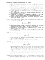
Designing the primary (master) loop. The closedloop characteristic equation for the
master loop is
l+-(l:g)=

l+(~)(s2+js+p)=0
(9.19)
5s3
+
16s2
+
ys
+
;
+ ;K2 = 0
(9.20)
Solving for the ultimate gain K, and ultimate frequency
w,
by substituting iw for
s
gives
K, = 30.8
co,,
=
,/5.1
= 2.26

It is useful to compare these values with those found for a single conventional control
loop, K, = 19.8 and
w,
= 1.61. We can see that cascade control results in higher con-
troller gain and a smaller closedloop time constant (the reciprocal of the frequency).
Therefore, the system will show faster response with cascade control than with a single
loop. Figure 9.2b gives a root locus plot for the primary controller with the secondary
controller gain set at
i.
Two of the loci start at the complex poles
s
=
-

$
5
ii
that
come from the clo;edloop secondary loop. The other curve starts at the pole
s
=
-

i.
n
306
fvwr

Two:
Laplace-Domain Dynamics and Control

Im
Kc=0
-2
-1
(a) Root locus for secondary loop
J
K2=0
X,=0
(6) Root ldcus for primary loop
Im
I
s
plane
-
Re
\
f
I‘Ku=
30.8
s plane
1
-
Re
FIGURE 9.2
(n) Root locus for secondary loop.
(b) Root locus for primary loop.
CHAPTER
Y:
Laplace-Domain Analysis of Advanced Control’Systems
307

9.1.2 Parallel Cascade
Figure
9.3~
shows a process where the manipulated variable affects the two con-
trolled variables
Yt
and
Y2
in parallel. An important example is in distillation col-
umn control where reflux flow affects both distillate composition and a tray temper-
ature. The process has a parallel structure, and this leads to a parallel cascade control
system.
If only a single controller
Gc~
is used to control
Yz
by manipulating
M,
the
closedloop characteristic equation is the conventional
1
+
G&m(s)
=
0
(9.21)
(a) Openloop process
(b)
Parallel cascade process
w

G,
(~1
Reduced block diagram
FIGURE 9.3
Parallel cascade. (a) Openloop
process.
(b)
Parallel cascade
control.
(c)
Reduced block
diagram.
308
PART TWO: Laplace-Domain Ilynamics and Control
If, however, a cascade control system is used, as sketched in Fig. 9.36, the closedloop
characteristic equation is not that given in Eq. (9.21). To derive it, let us start with
the secondary loop.
YI
= G,M = GIGc,(YF’
-

YI)
Y,
=
GIGCl

pet
1
+
GGCI

i
(9.22)
(9.23)
Combining Eqs. (9.22) and (9.23) gives the closedloop relationship between
M
and
UT”‘.
y,set
=
GCI
set
1
+
GIGI
Yl
(9.24)
Now we solve for the closedloop transfer function for the primary loop with the
secondary loop on automatic. Figure
9.3~
shows the simplified block diagram. By
inspection we can see that the closedloop characteristic equation is
(9.25)
Note the difference between the series cascade [Eq.
(9.4)]
and the parallel cascade
[Eq.
(9.25)]
characteristic equations.
9.2
FEEDFORWARD CONTROL

Most of the control systems we have discussed, simulated, and designed thus far
in this book have been feedback control devices. A deviation of an output variable
from a setpoint is detected. This error signal is fed into a feedback controller, which
changes the manipulated variable. The controller makes no use of any information
about the source, magnitude, or direction of the disturbance that has caused the output
variable to change.
The basic notion of feedforward control is to detect disturbances as they enter
the process and make adjustments in manipulated variables so that output variables
are held constant. We do not wait until the disturbance has worked its way through
the process and has upset everything to produce an error signal. If a disturbance
can be detected as it enters the process, it makes sense to take’immediate action to
compensate for
its effect on the process.
Feedforward control systems have gamed wide acceptance in chemical engi-
neering in the past three decades. They have demonstrated their ability to improve
control, sometimes quite spectacularly. The dynamic responses of processes that
have poor dynamics from a feedback control standpoint (high-order systems or
SYS-
terns with large deadtimes or inverse response) can often be greatly improved by
using feedforward control. Distillation columns are one of the most common ap-
plications of feedforward control. We illustrate this improvement in this section by
comparing the responses of systems using feedforward control with systems using
conventional feedback control when load disturbances occur.
3P
th
he
3Y
de
‘ar
)le

ch
on
ut
ter
es
d-l
ce
to
;i-
ve
iat
G-
bY
$I-
bY
“g
CIIAIT~:.K

9:
Laplace-Domain Analysis of Advanced Control Systems
309
Feedforward control is probably used more in chemical engineering systems
than in any other field of engineering. Our systems are often slow-moving, nonlinear,
and multivariable, and contain appreciable deadtime. All these characteristics make
life miserable for feedback controllers. Feedforward controllers can handle all these
with relative ease as long as the disturbances can be measured and the dynamics of
the process are known.
9.2.1 Linear Feedforward Control
A block diagram of ,a simple
openloop

process is sketched in Fig.
9.4~.
The load
disturbance
LQJ
and the manipulated variable
Mts,
affect the controlled variable
YQJ.
A conventional feedback control system is shown in Fig.
9.4b.
The error signal
I?(,)
is fed into a feedback controller
Gccs)
that changes the manipulated variable
MC,).
Figure
9.4~
shows the feedforward control system. The load disturbance
L+)
still
enters the process through the
GLqs)
p
recess transfer function. The load disturbance
is also fed into a feedforward control device that has a transfer function
GF(~).
The
feedforward controller detects changes in the load

Lt,,
and adjusts the manipulated
variable
Mt,).
Thus, the transfer function of a feedforward controller is a relationship between
a manipulated variable and a disturbance variable (usually a load change).
G
A4
F(s)
=
z
=
0
(
manipulated variable
disturbance
1
(9.26)
(4
Y constant
To design a feedforward controller, that is, to find
GF(~),
we must know both
GL(~)
and
GM(~).
The objective of most feedforward controllers is to hold the controlled
variable constant at its steady-state value. Therefore, the change or perturbation in
Yes)
should be zero. The output

Yc,)
is given by the equation
Y(s)
=
G~(s&(s)
+ %(s,M(s,
(9.27)
Setting
Yes,
equal to zero and solving for the relationship between
&Qs)
and
L+)
give
the feedforward controller transfer function.
(9.28)
EXAMPLE 9.2. Suppose we have a distillation column with the process transfer func-
tions
GMM(,~)
and
GLEN,
relating bottoms composition xg to steam flow rate
F,
and to feed
flow rate FL.
=
GM(s)
=
KM
T-MS+

1
=
CL(S)
=
KL
T/g
+ I
(9.29)
All these
variab1e.s
are perturbations from steady state. These transfer functions could
have been derived from a mathematical model of the column or found experimenrally.
3
IO
PAW

TWO
:
La$lace-Domain Dynamics and Control
(a) Openloop
=

GM(s)
Y(S)
c
(6) Feedback control
(c) Feedforward control
(4
Combined feedforward/feedback control
FIGURE 9.4

Block diagrams. (a) Openloop. (b) Feedback control. (c)
Feed-
forward control. (d) Combined feedforward/feedback control.
We want to use a feedforward controller G
F(~)
to make adjustments in steam flow to
the reboiler whenever the feed rate to the column changes, so that bottoms composition
is held constant. The feedforward controller design equation [Eq. (9.28)] gives
(&)

=

23

z
i

!
-

KLI(q,S

+

1)
-z‘&Qfs+
1
ZZ-
G
(19.30)

kf

(s)
KMI(7M.s

+
1)
KM

TLS

+

I
The feedforward controller contains a steady-state gain and dynamic terms. For this sys-
tem the dynamic element is a first-order lead-lag. The unit step response of this lead-lag
is an initial change to a
value
that is
(-

KLIKM)(~M/~L),
followed by an exponential rise
or decay
to
the final steady-state value
-

KL,IKM.
8

cf{AYfEK

9:
Laplace-Domain Analysis of Advanced Control Systems
311
The advantage of feedforward control over feedback control is that perfect con-
trol can, in theory, be achieved. A disturbance produces no error in the controlled
output variable if the feedforward controller is perfect. The disadvantages of feed-
forward control are:
1. The disturbance must be detected. If we cannot measure it, we cannot use feed-
forward control. This is one reason feedforward control for throughput changes is
commonly used, whereas feedforward control for feed composition disturbances
is only occasionally used. The former requires a flow measurement device, which
is usually available. The latter requires a composition analyzer, which is often not
available.
2.
We must know how the disturbance and manipulated variables affect the process.
The transfer functions
GL($)
and
GM(~)
must be known, at least approximately. One
of the nice features of feedforward control is that even crude, inexact feedforward
controllers can be quite effective in reducing the upset caused by a disturbance.
In practice, many feedforward control systems are implemented by using ratio
control systems, as discussed in Chapter 4. Most feedforward control systems are
installed as combined feedforward-feedback systems. The feedforward controller
takes care of the large and frequent measurable disturbances. The feedback controller
takes care of any errors that come through the process because of inaccuracies in the
feedforward controller as well as other unmeasured disturbances. Figure 9.4d shows

the block diagram of a simple linear combined feedforward-feedback system. The
manipulated variable is changed by both the feedforward controller and the feedback
controller.
For linear systems the addition of the feedforward controller has no effect on
the closedloop stability
,of
the system. The denominators of the closedloop transfer
functions are unchanged.
,
With feedback control:
Y(s)

=
Gw
‘G(s)

G(s)
1 +
G&c(s)
Lw
+
1 +
G~(s)Gc(s)
pet
(s)
With feedforward-feedback control:
Y(s)

=
GL(~)

+

G(s)Gqs)
4s)

+
GM(~)

G(s)
1

+

%(s)Gc(s)
1

+

Gw(s)Gc(s)
yss”,’
(9.3 1)
(9.32)
In a nonlinear system the addition of a feedforward controller often permits tighter
tuning of the feedback controller because it reduces the magnitude of the distur-
bances that the feedback controller must cope with.
Figure 9.5a shows a typical implementation of a feedforward controller. A dis-
tillation column provides the specific example. Steam flow to the reboiler is ratioed
to the feed flow rate. The feedforward controller gain is set in the ratio device. The
dynamic elements of the feedforward controller are provided by the lead-lag unit.

Figure
9.5b
shows a combined feedforward-feedback system where the feed-
back signal is added to the feedforward signal in a summing device. Figure
9.5~
.
^
. . . . , .
I

1
I

~

AC-
C
3
I2 PART TWO: Laplace-Domain Dynamics and Control
Feed
1
Ratio
+I
Ratio1
set
_I

Dynamic
elements
Steady-state

gain
element
Reboiler
Column
(a) Feedforward control
Feed
Lead-lag
Feedforward
Ratio
signal
\
Summer
Ratio
set
Column
I
I, /I
signal
I,
I/
I
Steam flow
(h) Feedforward-feedback control with additive signals
FIGURE 9.5
Feedforward systems.
CHAITEH

(I!
Laplace-Domain Analysis of Advanced Control Systems
3

13
Lead-lag
1
#

I
Steam
Column
3
(c) Feedforward-feedback control with feedforward gain modified
FIGURE 9.5 (CONTINUED)
Feedforward systems.
feedforward controller gain in the ratio device. Figure 9.6 shows a combined
feedforward-feedback control system for a distillation column where feed rate dis-
turbances are detected and both steam flow and reflux flow are changed to hold
constant both overhead and bottoms compositions. Two feedforward controllers are
required.
Figure 9.7 shows some typical results of using feedforward control. A
first-
order lag is used in the feedforward controller so that the change in the manipulated
variable is not instantaneous. The feedforward action is not perfect because the dy-
namics are not perfect, but there is a significant improvement over feedback control
alone.
It is not always possible to achieve perfect feedforward control. If the
GM(,)
transfer function has a deadtime that is larger than the deadtime in the
GL(~)
transfer
function, the feedforward controller will be physically unrealizable because it re-

quires predictive action. Also, if the
GM(~)
transfer function is of higher order than
the
GL(~)
transfer function, the feedforward controller will be physically unrealizable
[see Eq.
(9.28)].
9.2.2 Nonlinear Feedforward Control
There are no inherent linear limitations in feedforward control. Nonlinear feedfor-
ward controllers can be designed for nonlinear systems. The concepts are illustrated
in Example 9.3.
r
.
3 14
PART
TWO: Laplace-Domain Dynamics and Control
Feed
FIGURE 9.6
Combined feedforward-feedback system with two controlled variables.
EXAMPLE 9.3. The nonlinear
ODES
describing the constant-holdup. nonisothermal
CSTR system are
de/i
-=
dt
$CAO
-

CA)

-

C&w-E’RT
(9.33)
dT
dt=v
$0

-
T)
-

( +,cM-~‘~~

-

($$(I

-

T,>
(9.34)
Let us choose a feedforward control system that holds both reactor temperature T
and reactor concentration
CA
constant at their steady-state values, T and
CA.
The feed

flow rate F and the jacket temperature
TJ
are the manipulated variables. Disturbances
are feed concentration
CAO
and feed temperature
TO.
Noting that we are dealing with total variables now and not perturbations, the feed-
forward control objectives are
c
A(f)
=
c,
and
Tct,
=
r
Substituting these into Eqs. (9.33) and (9.34) gives
(9.35)
.a1
3)
4)
T
:d
es
d-
5)
6)
CHAITEKY: Laplace-Domain Analysis of Advanced Control! Systems
3 15

m
Feedforward
*
Time
Feedback
*
*
Time
FIGURE 9.7
Feedforward control performance for load disturbance.
dT
F(r)
dt
= 0 =
+Tot,)

-
T)
-
-

(-&-)cJ

-

($-JF

-

73

-?9.37)
Rearranging Eq. (9.36) to find
F,,,,
the manipulated variable, in terms of the disturbance
CAO(~)
gives the nonlinear feedforward controller relating the load variable
CA0
to the
manipulated variable F.

F(r)
=
CAkV
CAO(r)
-

c*
(9.38)
The relationship is hyperbolic, as shown in Fig. 9.8. Feed rate must be decreased as feed
concentration increases. This increases the holdup time, with constant volume, so that
the additional reactant is consumed. Equation (9.38) tells us that feed flow rate does not
have to be changed when feed temperature
TO
changes.
Substituting Eq. (9.38) into Eq. (9.37) and solving for the other manipulated variable
TJ
give
C(I)
=T+

C,(T

-

TO(l)>
cAO(r)
-

CA
1
(9.39)
This is a second nonlinear feedforward relationship that shows how cooling-jacket tem-
perature
TJ(,)
must be changed as both feed concentration
CAocr)
and feed temperature
To(,)
change. Notice that the relationship between
TJ
and
CA0
is nonlinear, but the rela-
tionship between
TJ
and
To
is linear.
a
3

I6
PART TWO: Laplace-Domain Dynamics and Control
controller
Feed concentration
CAO(,)
FIGURE 9.8
Nonlinear relationship between feed rate and feed concentration.
The preceding nonlinear feedforward controller equations were found analy-
tically. In more complex systems, analytical methods become too complex, and
numerical techniques must be used to find the required nonlinear changes in ma-
nipulated variables. The nonlinear steady-state changes can be found by using the
nonlinear algebraic equations describing the process. The dynamic portion can often
be approximated by linearizing around various steady states.
9.3
OPENLOOP-UNSTABLE PROCESSES
We remarked earlier in this book that one of the most interesting processes that chem-
ical engineers have to control is the exothermic chemical reactor. This process can
be
openloop
unstable.
Openloop instability means that reactor temperature will take off when there is
no feedback control of cooling rate. It is easy to visualize qualitatively how this can
occur. The reaction rate increases as the temperature climbs and more heat is given
off. This heats the reactor to an even higher temperature, at which the reaction rate
is still faster and even more heat is generated.
There is also an openloop-unstable mechanical system: the inverted pendulum.
This is the problem of balancing a stick on the palm of your hand. You must keep
moving your hand to keep the stick vertical. If you put your brain on manual and
hold your hand still, the stick topples over. So the process is
openloop

unstable. If
you think balancing an inverted pendulum is tough, try controlling a double inverted
pendulum (two sticks on top of each other). You can see this done using a feedback
controller at the French Science Museum in Paris.
We explore the effects of
openloop
instability quantitatively in the
s
plane.
We discuss linear systems in which instability means that the reactor temperature
theoretically goes to infinity. Because any real reactor system is nonlinear, reactor
temperature will not increase without bounds. When the concentration of reactant
begins to drop, the reaction rate eventually slows down. However, before it gets to
(YIAIWK

o:

Laplace-Domain
Analysis of Advanced
Contt.ol
Systems
317
that point the reactor may have blown a rupture disk or melted down! Nevertheless,
linear techniques are very useful in looking at stability near some operating level.
Mathematically, if the system is
openloop
unstable, its
openloop
transfer function
G,,J(.~J

has at least one pole in the RHP.
9.3.1 Simple Systems
As a simple example, let us look at just the energy equation of the nonisothermal
CSTR process of Example 7.6. We neglect any changes in
CA
for the moment.
dT
-
=
aTaT

-I-

a26TJ

+

*.

-
dt
Laplace transforming gives
(S

-

n22)T(.s)
= 026T.Q) +
*

-

-
T(,s,

=
a26
s

-
a22
TJ(,) + . . .
(9.40)
(9.41)
Thus, the stability of the system depends’on the location of the pole
a22.
If this pole
is positive, the system is
openloop
unstable. The value of
a22
is given in Eqs. (7.82).
-AkEC/,

F
UA
a22 =
-_
pC,RT2
v

VPC,
For the system to be
openloop
stable,
a22

<
0.
-AkEc/,
F UA
<o
-

pC,RT2
’
VP%
-hkEi?/,

<‘+

UA
PC,
RT2
v

VPC,
(9.42)
The left side of Eq. (9.43) represents the heat generation due to reaction. The right
side represents heat removal due to sensible heat and the heat transfer to the jacket.
Thus, our simple linear analysis tells us that the heat removal capacity must be

greater than the heat generation if the system is to be stable. The actual stabil-
ity requirement for the nonisothermal CSTR system is a little more complex than
Eq. (9.43) because the concentration
CA
does change.
A. First-order openloop-unstable process
Suppose we have a first-order process with the
openloop
transfer function
(9.44)
Note that this is
not
a first-order lag because of the negative sign in the denominator.
The system has an
openloop
pole in the RHP at
s
= +
l/r,.
The unit step response
I-
.I .
:

,.I
l-l

*

P

*>
:

~
318

PART
~hvo:
Laplace-Domain Dynamics and Control
Can we make the system stable by using feedback control‘? That is, can an
openloop-unstable process be made closedloop stable by appropriate design of the
feedback controller? Let us try a proportional controller:
Gc(sj
=
K,
The closedloop
characteristic equation is
1
+
G~(s)Gc(s)
=
1
+
KP
r

s
_
l

Kc
=
0
0
s =
I

-
K,K,,
70
There is a single closedloop root. The root locus plot is given in Fig. 9.9a. It starts at
the openloop pole in the RHP. The system is closedloop unstable for small values of
controller gain. When the controller gain equals
l/K,,
the closedloop root is located
right at the origin. For gains greater than this, the root is in the LHP, so the system
is closedloop stable.
Thus, in this system there is a minimum stable gain. Some of the systems studied
up to now have had maximum values of gain
K,,,
(or ultimate gain K,,) beyond
which the system is closedloop unstable. Now we have a case that has a minimum
gain
Kmin
below which the system is closedloop unstable.
vp
(a) First-order:
GC(sjGMcs,=

-g-q
0
Kc
= 0
I

.
1
5
0
I
w
s plane
Kc
= 0
t
s
plane
Kc=+
P
*
K,.=O
\,
I\
I
-
roz
+a
‘00
K,.

Kp
= (q,,s
+

1)(2(,7
I)
FIGURE
9.9
Root locus curves for openloop unstable processes (positive
poles).
m
le
‘P
5)
at
of
zd
m
zd
lzd
.m
~~IIAIWK

9:
Laplace-Domain Analysis of Advanced Control Systems
3
19
W

K,.
-+
00
(Closedloop unstable
A
for all
K,.)
Kc = 0
\I
/\
*
I

7
0 I
s plane
K<
= 0
(c)

701

’
702
s
plane
s
plane
+$
02

(d) Third-order:
Gccs,GMc,,
=
Kc&
(74x+

l)(z,*s+

1)(7,3s-

1)
FIGURE 9.9 (CONTINUED)
Root locus curves for openloop unstable processes (positive poles).
B. Second-order openloop-unstable process
Consider the process given in Eq. (9.44) with a first-order lag added.
(9.46)
One of the roots of the
openloop
characteristic equation lies in the RHP at
s
=
+
l/7,2.
Can we make this system closedloop stable? A proportional feedback controller
gives a closedloop characteristic equation:
1

+

%.f(.Y)GC(.V)

=

1

+
4,
(TOIS +
wo2s

-
1)
K,.
= 0
320
PAKTTWO:

~~l~~~lce-~~~~ll~lill
~)‘ll~llllicS Uld
&ltrOi
Two conditions must be satisfied if there are to be no positive roots of this
closedloop
characteristic equation:
(9.48)
Therefore, if
7,2
<
7,1
a proportional controller cannot make the system closedloop
stable. A controller with derivative action might be able to stabilize the system. Fig-

ures
9.9b
and c give the root locus plots for the two cases
7,~

>

~~1
and
7,2
<
~~1.
In
the latter case there is always at least one closedloop root in the RHP, so the system
is always unstable.
C. Third-order openloop-unstable process
‘If an additional lag is added to the system and a proportional controller is used,
the closedloop characteristic equation becomes
1

+

Gv(s)Gc(s)

=

1

+
KIJ

(GlS
+
M702s
+
1)(703s

-

1)
K, = 0
(9.49)
Figure 9.9d gives a sketch of a typical root locus plot for this type of system. We now
have a case of conditional stability. Below
Kmin
the system is closedloop unstable.
Above
K,,,
the system is again closedloop unstable. A range of stable values of
controller gain exists between these limits:
Kmin

<

Kc

<

Kmax
(9.50)
Clearly, the closer the values of

K,,,
and
Kmin
are to each other, the less controllable
the system will be.
EXAMPLE 9.4. The transfer function relating process temperature T to cooling-water
flow rate
F,
in an openloop-unstable chemical reactor is
G
-0.7 (“F/gpm)
M(s) =
(3
+ 1)(7s
-
1)
(9.5 1)
where the time constants 1 and
T
are in minutes. The temperature measurement has a
dynamic first-order lag of 30 seconds. The range of the analog electronic (4 to 20 mA)
temperature transmitter is 200 to 400°F. The control valve on the cooling water has Iinear
installed characteristics and passes 500 gpm when wide open. The temperature controller
is proportional.
(a) What is the closedloop characteristic equation of the system?
We must include the OS-minute lag of the temperature transmitter and the gains for
both the transmitter and the valve.
1

+

G~(.~)G~(s)Gv(s)Gc(s)
=
o
Note that the gain of the controller is chosen to be positive (reverse acting), so the con-
troller output decreases as temperature increases, which increases cooling-water flow
through the AC valve (this makes the gain of the control valve negative).
(0.ST).S3

+

(I.57

-

0.S).s2

+
(7
-
l.S)s +
(1.7SK,.

-

I)
= 0
(9.52)
‘P
d,

er
3r
(YIAIVIJK

V:
Laplace-Dotnnin Analysis of Advanced Control Systems
321
(h) What is the minimum value of controller gain,
K,,in,
that gives a closedloop-stable
system?
Letting s =
io
in Eq. (9.52) gives two equations in two unknowns:
Kc
and w.
From the real part:
0.5~~
-
1.50% +
l.75K,

-
I = 0
From the imaginary part:
WT

-
1.50
-

0.5TW
3’0
There are two solutions for Eq. (9.54):
(9.53)
(9.54)
J
7

-
I.5
w=Oandw=

___
0.57
(9.55)
Using
w
= 0 gives the minimum value of gain.
I
Kmin

=

-
1.75
(c) Derive a relationship between
T
(the positive pole) and the maximum closedloop
stable gain,

K,,,.
Using the second value of
w
in Eq. (9.55) gives
K,,,.
Llax =
1.5
-

4.57

+
3T2
1.757
(9.56)
(d) Calculate K,,,,
when
T
= 5 minutes and 10 minutes.
For
T
= 5,
K,,,
= 6.17
For
T
=
10,
K,,,
= 14.7

Note that this result shows that the smaller the value of T (i.e., the closer the positive pole
is to the value of the negative poles:
s
=
-
1 and
-2),
the more difficult it is to stabilize
the system.
(e) At what value of T will a proportional-only controller be unable to stabilize the
system?
When
K,,,
=
Kmin
the system will always be unstable.
1.5
-
4.57

f
3T2
1
=
-
=
1.757
I.75
3
7

1.5
minutes
Note that there are actually two values of
T
that satisfy the equation above, but the lim-
iting one is the larger of the two.
9.3.2 Effects of Lags
The systems explored in the preceding section illustrate a very important point about
the control of openloop-unstable systems: The control of these systems becomes
more difficult as the order of the system is increased and as the magnitudes of the
first-order lags increase. Our examples demonstrated this quantitatively. For this rea-
son, it is vital to
design
a reactor control system with very fast measurement d~nnm-
its and very fast heat removal dynamics. If the thermal lags in the temperature sensor
322
PARTTWO:
Laplace-Domain Dynamics and Control
and in the cooling jacket are not small, it may not be possible to stabilize the reactor
with feedback control. Bare-bulb thermocouples and oversized cooling-water valves
are often used to improve controllability.
9.3.3 PD Control
Up to this point we have looked at using proportiona
unstable systems. Controllability can often be improved
in the controller. An example illustrates the point.
.l
controllers on openloop-
by using derivative action
EXAMPLE 9.5. Let us take the same third-order process analyzed in Example 9.4. For
T

= 5 minutes and a proportional controller, the ultimate gain was 6.17 and the ultimate
frequency was 1.18 rad/min.
Now we use a PD controller with
~0
set equal to 0.5 minutes (just to make the
algebra work out nicely; this is not necessarily the optimal value of
7~).
The closedloop
characteristic equation becomes
1.75
1
TgS
+ 1
(S
i
I)(%
-
l)(o.% +
1)

Kc
0.17~s +
1
=
’
(9.57)
o.25s3
+
5.2s*
+ 3.95s + 1.75K,

-
1 = 0
Solving for the ultimate gain and frequency gives
KU
= 47.5 and
o,
= 3.97. Comparing
these with the results for P control shows a significant increase in gain and reduction in
closedloop time constant.
9.3.4 Effect of Reactor Scale-up on Controllability
One of the classical problems in scaling up a jacketed reactor is the decrease in the
ratio of heat transfer area to reactor volume as size is increased. This has a profound
effect on the controllability of the system. Table 9.1 gives some results that quan-
tify the effects for reactors varying from 5 gallons (typical pilot plant size) to 5000
gallons. Table 9.2 gives parameter values that are held constant as the reactor is
scaled up.
TABLE 9.1
Effect of scale-up on controllability
Reactor volume (gal)
5
500 5ooo
Feed rate (Ib,,,/hr) 27.8 2780
27,800
Heat transfer ( 1
O6
BtuIhr)
0.0028 0.28
2.8
Reactor height (ft)
1

SO4 6.98
15.04
Reactor diameter (ft)
0.752 3.49
7.52
Heat transfer area (ft2) 3.99 86.15
400
Cooling-water flow (gpm) 0.086
11.58
240
Jacket (“F)
temperature
135.3 118.3
93.3
Controller- gains
MltX
169 100 144
b4;,,
I
77
I
nc
n

Al
(~IIAI&X

o:

Laplace-Domain

Analysis of Advanced Control Systems
323
‘I’AIlLE
Y.2
Reactor parameters
Reactor
lwldup

time
Jacket holdup time
Overall heat transfer coefficient
Heat capacity of products and feeds
Heat capacity of cooling water
Density of products and feeds
Density of cooling water
Inlet cooling-water temperature
Temperature measurement lag
Feed concentration
Feed temperature
Reactor temperature
Preexponential factor
Activation energy
Heat of reaction
Steady-state concentration
Specific reaction rate
Temperature transmitter span
Cooling-water valve maximum flow rate
1.2 h
0.077 h
I.50

Btu/h

ft*

“F
0.75
Btu/lb,,,

“F
I
.O Btu/lb,,,
“F
50
Ib,,/ft’
62.3
Ib,,/f+
70°F
30 s
0.50 lb-mol A/ft”
70°F
140°F
7.08 x
IO’O

h-’
30,000 Btu/lb-mol
-30,000
Btu/lb-mol
0.245 lb-mol A/ft3

0.8672 h-’
100°F
Twice normal design flow rate
Notice that the temperature difference between the cooling jacket and the reactor
must be increased as the size of the reactor increases. The flow rate of cooling water
also increases rapidly as reactor size increases.
The ratio of
K,,,
to
Kmi”,
which is a measure of the controllability of the system,
decreases from 124 for a Sgallon reactor to 33 for a
5000-gallon
reactor.
9.4
PROCESSES WITH INVERSE RESPONSE
Another interesting type of process is one that exhibits inverse response. This phe-
nomenon, which occurs in a number of real systems, is sketched in Fig.
9.10b.
The
response of the output variable
yo)
begins in the direction opposite of where it fin-
ishes. Thus, the process starts out in the wrong direction. You can imagine what this
sort of behavior would do to a poor feedback controller in such a loop. We show
quantitatively how inverse response degrades control loop performance.
An important example of a physical process that shows inverse response is the
base of a distillation column with the reaction of bottoms composition and base level
to a change in vapor
boilup.

In a binary distillation column, we know that an increase
in vapor
boilup
V must drive more low-boiling material up the column and therefore
decrease the mole fraction of light component in the bottoms xg. However, the tray
hydraulics can produce some unexpected results. When the vapor rate through a tray
is increased, it tends to (1) back up more liquid in the downcomer to overcome the
increase in pressure drop through the tray and (2) reduce the density of the liquid
and vapor froth on the active part of the tray. The first effect momentarily reduces
the liquid flow rates through the column while the liquid holdup in the downcomer is
324
IMTTWO:

Laplace-Dolnain
Dynamics and Control


_-
T
I
*

t
K2
s plane
2
Cc)
FIGURE 9.10
Process with inverse response. (n) Block diagram. (b) Step response.
(c)

Root locus plot.
building up. The second effect tends to momentarily increase the liquid rates since
there is more height over the weir.
Which of these two opposing effects dominates depends on the tray design and
operating level. The pressure drops through valve trays change
iittle
with vapor rates
unless the valves are
cotioletrlv

lifted

Therefnre

thP

c~rnd
pffant
;c

o, mn+;m,~
since
n and
rates
times
”
Gent
increase in liquid rates down the column. This increase in liquid rates carries material
that is richer in light component into the reboiler and momentarily increases
x0.

Eventually, of course, the liquid rates will return to normal when the liquid inventory
on the trays has dropped to the new steady-state levels. Then the effect of the increase
in vapor
boilup
will drive xn down. Thus, the vapor-liquid hydraulics can produce
inverse response in the effect of V on xg (and also on the liquid holdup in the base).
Mathematically, inverse response can be represented by a system that has a
transfer function with a positive zero, a zero in the RHP. Consider the system
sketched in Fig. 9.1 Oa. There are two parallel first-order lags with gains of opposite
sign. The transfer function for the overall system is
Ws)
If the K’s and
the system will
rearranged as
701s
+
1
702s +
1
0’s
are such that
ro2
>
-
>
1
K2
-
701

KI
show inverse response, as sketched in Fig.
9.10b.
Eq. (9.58) can be
(9.59)
Thus, the system has a positive zero at
K2

-

&
s
=
K&2

-

Kg,,
Keep in mind that the positive zero does not make the system
openloop
unstable.
Stability depends on the poles of the transfer function, not on the zeros. Positive
zeros in a system do, however, affect
cZosedoop
stability, as the following example
illustrates.
EXAMPLE 9.6. Let us take the same system used in Example 8.7 and add a positive
zeroats = ++.
G
-3s+

1
M(s)
= (s
+
l)(Ss +
1)
With a proportional feedback controller the closedloop characteristic equation is
1
+ G~(.Jkys) =
1
+
-3s+
1
(s
+

1)(5s
+
l)Kc
(9.60)
(9.61)
5s2
+ (6
-
3K,)s + 1
-t-

Kc
= 0
The root locus curves are shown in Fig. 9.10~. The loci start at

the.
poles of the open-
loop transfer function: s =
-
1 and s =
-

i.
Since the loci must end at the zeros of the
openloop
transfer function
(s
= +
f),
the curves swing over into the RHP. Therefore, the’
system is closedloop unstable for gains greater than 2.
Remember that in Example 8.8 adding a lead or a negative zero made the closedloop
system more stable. In this example we have shown that adding a positive zero has the
reverse effect.
a
326 MKTTWO: Laplace-Domain Dynamics and Control
9.5
MODEL-BASED CONTROL
Up to this point we have generally chosen a type of controller
(P,
PI, or PID) and
determined the tuning constants that gave some desired performance (closedloop
damping coefficient). We have used a model of the process to calculate the con-
troller settings, but the structure of the model has not been explicitly involved in the
controller design.

There are several alternative controller design methods that make more explicit
use of a process model. We discuss two of these here.
9.5.1 Direct Synthesis
In direct synthesis the desired closedloop response for a given input is specified.
Then, with the model of the process known, the required form and tuning of the
feedback controller are back-calculated. These steps can be clarified with a simple
example.
EXAMPLE 9.7. Suppose we have a process with the openloop transfer function
(9.62)
where
KP
and
rO
are the openloop gain and time constant. Let us assume that we want
to specify the closedloop servo transfer function to be
$-

1
TZ
-

~
7,s
+ 1
(9.63)
That is, we want the process to respond to a step change in setpoint as a first-order process
with a closedloop time constant
rc.
The steady-state gain between the controlled variable
and the setpoint is specified as unity, so there will be no offset.

Now, knowing the process model and having specified the desired closedloop servo
transfer function, we can solve for the feedback controller transfer function
Gccs).
We
define the closedloop servo transfer function as
Scs).
yw
S(s)

=

yset

=
GwGc(s)
(s)
1

+

Gw%s,
(9.64)
Equation (9.64) contains only one unknown (i.e., the feedback controller transfer func-
tion
Gccsj).
Solving for G
c(~)
in terms of the known values of
G,,!,,,
and

ScsJ
gives
(9.65)
Equation (9.65) is a general solution for any process and for any desired closedloop servo
transfer function. Plugging in the values for
G,,,,($)
and
Sts,
for the specific example gives
I
G-(x)
=
T(.S

+

1
T,S +
1
VIIAI~XK

9:
Laplace-Domain Analysis of Advanced Control Systems
327
Equation (9.66) can be rearranged to look just like a PI controller if
K,.
is set equal to
r,,/~,
K,, and the
rcsct

time
T/
is set equal to
T,,.
r/s + I
Gcc,y)
=
Kc

-
=
71s
(9.67)
Thus, we find that the appropriate structure for the controller is PI, and we have solved
analytically for the gain and reset time in terms of the parameters of the process model
and the desired closedloop response.
Before we leave this example, it is important to make sure that you understand the
limitations of the method. Suppose the process
openloop
transfer function also contained
a deadtime.
KKD”
GM(s)

=

___
7,s

+

1
Using this
GM~,~)
in Eq. (9.65) gives a new feedback controller:
G(s)

=
(7,s

+

I)e+DS
K&S
(9.68)
(9.69)
This controller is not physically realizable. The negative deadtime implies that we can
change the output of the device
D
minutes before the input changes, which is impossible.
This case illustrates that the desired closedloop relationship cannot be chosen arbi-
trarily. You cannot make a jumbo jet behave like a jet fighter, or a garbage truck drive
like a Ferrari! We must select the desired response so that the controller is physically
realizable. In this case all we need to do is modify the specified closedloop servo trans-
fer function
So)
to include the deadtime.
(9.70)
Using this
Scs)

in Eq. (9.65) gives exactly the same
G,-cs)
as found in Eq. (9.66), which
is physically realizable.
As an additional case, suppose we had a second-order process transfer function.
KP
Gm

=

(Tos

+

1)2
Specifying the original closedloop servo transfer function [Eq. (9.63)] and solving for
the feedback controller using Eq. (9.65) gives
Gee;,

=
!‘(” + ‘j2
5
K,m
Again, this controller is physically unrealizable because the order of the numerator is
greater than the order of the denominator. We would have to modify our specified S,,, to
make this controller realizable. n
This type of controller design has been around for many years. The “pole place-
ment” methods used in aerospace systems employ the same basic idea: the controller
is designed to position the poles of the closedloop transfer function at the desired lo-
cation in the s plane. This is exactly what we do when we specify the’closedloop

time constant in Eq. (‘3.63).
9.5.2 Internal Model Control
Garcia and
Moral-i

(lnd.

Eq.
Chcm.

Pt-oce.ss
Des.
Dev.
21: 308, 1982)
have used a
similar approach in developing “internal model control” (IMC). The method gives
the control engineer a different perspective on the controller design problem. The
basic idea of IMC is to use a model of the
openloop
process
GMM(.~J
transfer function in
such a way that the selection of the specified closedloop response yields a physically
realizable feedback controller.
Figure 9.11 gives the IMC structure. The model of the process
GM(~)
is run in
parallel with the actual process. The output of the model
Y
is subtracted from the

actual output of the process Y, and this signal is fed back into the controller
GIMC(~).
If our model is perfect (G
M
=
GM),
this signal is the effect of load disturbance on
the output (since we have subtracted the effect of the manipulated variable M). Thus,
we are “inferring” the load disturbance without having to measure it. This signal is

1
Model
(a) Basic structure
r
_-_
1
:+a

-@
,
y=
1
-_
-J
‘Traditional
G,
(b) Reduced structure
FIGURE
9.11
IMC.