Essentials of Process Control phần 5 pps

7)
Id
8)
f
cIwrf:K
7:
Laplace-Domain Dynamics
237
B = lim
K,‘tT:
4)
___
=

Therefore,
I
l/T,
1
;

-

(s
+ 1/T,)2
-
s
+
l/T”
Inverting term by term yields
7.4
TRANSFER FUNCTIONS

Our primary use of Laplace transformations in process control involves representing
the dynamics of the process in terms of “transfer functions.” These are output-input
~~~
relationships and are obtained by Laplace-transforming algebraic and differentktl
equations. In the following discussion, the output variable of the process is
~(~1.
The
~~~~
input variable or the forcing function is
~(~1.
7.4.1 Multiplication by a Constant
Consider the algebraic equation
Y(t)
=
KU(t)
(74lj~~

mm
Laplace-transforming both sides of the equation gives
I
02 cc
o

Ywe
-dt
=
K
i
tqt)P’

dt
0
Y(Y)
=
KU(s)
(7.42)
where
YtS,
and
Ut,)
are the Laplace transforms of y& and
~(~1.
Note that
U(Q
is an
arbitrary function of time. We have not specified at this point the exact form of the
input. Comparing Eqs. (7.41) and (7.42) shows that the input and output variables
~~
are related in the Laplace domain in exactly the same way as they are related in the
time domain. Thus, the English and Russian words describing this situation are the
same.
Equation (7.42) can be put into transfer function form by finding the outputiinput
ratio:
Y(.d
_ K
__

-
U(s)
(7.43)

238 PARTTWO:
Laplace-Domain
Dynamics and Control
%)
-v(f)
*

‘Time
domain
*

Laplace
domain
FIGURE 7.2
Gain transfer function.
For any input
UcS)
the output
Y(,,
is found by simply multiplying
Ucs)
by the constant
K. Thus, the transfer function relating
YtS,
and
Uc,y,
is a constant or a “gain.” We can
represent this in block-diagram form as shown in Fig. 7.2.
7.4.2 Differentiation with Respect to Time
Consider what happens when the time derivative of a function

‘ytt)
is Laplace trans-
formed.
Integrating by parts gives
(7.44)
u
=
p
dv =
2dt
dt
du =
-sedsf
dt v=y
Therefore,
-st
dt =
[yC’]::;
+
sye ”
dt
I-
a
=

0

-

Y(t=O)

+ s
Y(t)e-

dt
o
The integral is, by definition, just the Laplace transformation of
ycr),
which we call
Y(s).
=

sq,,

-

Y(f=O)
(7.45)
The result is the most useful of all the Laplace transformations. It says that the op-
eration of differentiation in the time domain is replaced by multiplication by s in
the Laplace domain, minus an initial condition. This is where perturbation variables
become so useful. If the initial condition is the steady-state operating level, all the
initial conditions like
Y(~=o)
are equal to zero. Then simple multiplication by
s
is
equivalent to differentiation. An ideal derivative unit or a perfect differentiator can
be represented in block diagram form as shown in Fig. 7.3.
The same procedure applied to a second-order derivative gives
2

=

s2
Y,,)
-
sy(, =())
-
(7.46)
1
>
CIIAWI:.K

7:

Laplace-IXtnain

Dynatnics
239
Y(s)
SY(,,
+

Laplace
domain
42
Time domain
Y(s)
2Y(s)
*

Laplace
domain
FIGURE 7.3
Differential transfer function.
Thus, differentiation twice is equivalent to multiplying twice by
S,
if all initial con-
ditions are zero. The block diagram is shown in Fig. 7.3.
The preceding can be generalized to an Nth-order derivative with respect to
time. In going from the time domain into the Laplace domain,
dNxldtN
is replaced
by
sN.
Therefore, an Nth-order differential equation becomes an Nth-order algebraic
equation.
dNY
dN-’
y
‘IN

dtN
-

+

aN-l-
dY
dtN-’
+ . . .

+
al

dt
+
a0y
=
U(t)
(7.47)
aNsN

Y(s)

+

aN-

1s
N-‘Y@)
+
**-
+‘a&,)
+
a0Y(,)
=
&)
(7.48)
(aNsN

+

aN-lsNel

+

”

’

+

als

+

aO>Y(,)

=

u(s)
(7.49)
Notice that the polynomial in Eq. (7.49) looks exactly like the characteristic equa-
tion discussed in Chapter 2. We return to this not-accidental similarity in the next
section.
7.4.3 Integration
Laplace-transforming the integral of a function
yet)
gives
Integrating by parts,
u

=
J
ydt
dv = e ” dt
du =
ydl
1
”
=
e s’
s
240
PAW TWO: Laplace-Domain Dynamics and Control
Y(l)
IY(,#f
+
Time domain
t
I
;

Y(.s,
s
=-
Laplace
dolnain
FIGURE 7.4
Integration transfer function.
Therefore,
2

if
1
y(,)dt
=
‘Y
+
A
s
w
s
(7.50)
The operation of integration is equivalent to division by s in the Laplace domain,
using zero initial conditions. Thus integration is the inverse of differentiation. Fig-
ure 7.4 gives a block diagram representation.
The l/s is an operator or a transfer function showing what operation is performed
on the input signal. This is a completely different idea from the simple Laplace trans-
formation of a function. Remember, the Laplace transform of the unit step function
is also equal to l/s. But this is the Laplace transformation of a function. The l/s
operator discussed above is a transfer function, not a function.
7.4.4
Deadtime
Delay time, transportation lag, or deadtime is frequently encountered in chemical en-
gineering systems. Suppose a process stream is flowing through a pipe in essentially
plug flow and that it takes D minutes for an individual element of fluid to flow from
the entrance to the exit of the pipe. Then the pipe represents a deadtime element.
If a certain dynamic variable fit,, such as temperature or composition, enters the
front end of the pipe, it will emerge from the other end
D
minutes later with exactly
the same shape, as shown in Fig. 7.5.

pp,
FIGURE

,.5
t=O
t=D
Effect of a dead-time element.
cItAfTER

7:
Laplace-Domain Dynamics
241
-
Time domain
Laplace domain
FIGURE 7.6
Deadtime transfer function.
Let us see what happens when we Laplace-transform a function
h,-o,
that has
been delayed by a deadtime. Laplace transformation is defined in Eq. (7.5 1).
af,,,1

=
I
Y
(@I

dt
=

F(s)
o
(7.5
1)
The variable
t
in this equation is just a “dummy variable” of integration. It is inte-
grated out, leaving a function of only
s.
Thus, we can write Eq. (7.5 1) in a completely
equivalent mathematical form:
(7.52)
where y is now the dummy variable of integration.
Now
let y =
t

-

D.
F(s)

=
I
m

fit-&
SO D)

d(t

-

0)

=

p
m

fit-D,e-“’
dt
0
f
0
(7.53)
F(,)
=
eD”3Lf&d
Therefore,
%ht-o)l
=
e-DsFcs)
(7.54)
Thus, time delay or deadtime in the time domain is equivalent to multiplication by
eeDS
in the Laplace domain.
If the input into the deadtime element is
~(~1
and the output of the deadtime

element is y(+ then
u
and y are related by
Y(f) =
q-D)
And in the Laplace domain,
Y(,)
=
e
-Ds
4)
(7.55)
Thus, the transfer function between output and input variables for a pure deadtime
process is
epDS,
as sketched in Fig. 7.6.
7.5
EXAMPLES
Now we are ready to apply all these Laplace transformation techniques to some typ-
ical chemical engineering processes.
I
242
PARTTWO:
Laplace-Domain Dynamics and Control
E
x
A M
P
I
,

E

7.3.
Consider the isothermal CSTR of Example 2.6. The equation describing
the system in terms of perturbation variables is
-
+
L
+ k
CiCn
dt
i

1
7
CA(,)
=
L

CAOW
7
(7.56)
where k and
r
are constants. The initial condition is
CA(o)
= 0. We do not specify what
Cnocr,
is for the moment, but just leave it as an arbitrary function of time. Laplace-
transforming each term in Eq. (7.56) gives

scA(s)

-

CA(t=O)
+
(7.57)
The second term drops out because of the initial condition. Grouping like terms in
CA($)
gives
Thus, the ratio of the output to the input (the “transfer function”
Cc,,)
is
%s)
Gtsj

zz

-
=
l/r
CAO(s)
s+k+

l/r
(7.58)
The denominator of the transfer function is exactly the same as the polynomial in
s
that was called the characteristic equation in Chapter 2. The roots of the denominator of
the transfer function are called the poles of the transfer function. These are the values of

s at which
Gc,,
goes to infinity.
The roots of the characteristic equation are equal to the poles of the transfer function.
This relationship between the poles of the transfer function and the roots of the charac-
teristic equation is extremely important and useful.
The transfer function given in Eq. (7.58) has one pole with a value of
-(k
+
l/r).
Rearranging Eq. (7.58) into the standard form of Eq. (2.51) gives
G(,)

=
s+l
6
=-
7,s + 1
(7.59)
where
K,
is the process steady-state gain and
r,,
is the process time constant. The pole
of the transfer function is the reciprocal of the time constant.
This particular type of transfer function is called a
jrst-order
lag. It tells us how
the input
CAO

affects the output
C
A,
both dynamically and at steady state. The form of
the transfer function (polynomial of degree 1 in the denominator, i.e., one pole) and the
numerical values of the parameters (steady-state gain and time constant) give a com-
plete picture of the system in a very compact and usable form. The transfer function
is a property of the system only and is applicable for any input. We can determine the
dynamics and the steady-state characteristics of the system without having to pick any
specific forcing function.
If the same input as used in Example 2.6 is imposed on the system, we should be
able to use Laplace transforms to find the response of
CA
to a step change of magni-
-
tude
CAM.
:
:-
).
U
le
kv
,f
ke
l-
In
le
‘Y
)e

i-
CtIAtTtiK
7: Laplace-Domain Dynamics
243
We take the Laplace transform of
Cncy,,,
substitute into the system transfer function,
solve for
CA(,~),
and invert back into the time domain to find
CA(,).
~e[cAO,,,l
=
CA(@)
=
r,O;
(7.61)
(7.62)
Using partial fractions expansion to invert (see Example 7.1) gives
C
n(t)
=
K,C,q)
(1
-

e-y
This is exactly the solution obtained in Example 2.6 [Eq. (2.53)].
n
EXAMPLE 7.4. The ODE of Example 2.8 with an arbitrary forcing function

uct)
is
d2y
dy
-
+
5&
+ 6y =
u(t)
dt2
with the initial conditions
(7.63)
(7.64)
Laplace transforming gives
s2

Y(s)
+
5q,,
+ 6Y(,, =
u(s)
YG)(s3
+ 5s + 6) =
U(s)
The process transfer function
Gcs)
is
s
=
GcS)

=
s2
+
;,
+
6
=
1
4s)
(s +
2)(s
+ 3)
Notice that the denominator of the transfer function is again the same polynomial in
s as appeared in the characteristic equation of the system [Eq. (2.73)]. The poles of the
transfer function are located at
s
= -2 and s = -3. So the poles of the transfer function
are the roots of the characteristic equation.
If
uct)
is a ramp input as in Example 2.13,
(7.66)
Y(s)

=

G(s)

U(s)

=
(,+:,ih)(~)=

s2(s+:)(s+3)
Partial fractions expansion gives
AB C
Y(s)
=
p

+

;
+
-
s
i-
2
A
=
li$

,s2

YW
i

i
= lim
e-+0

B = lim
s-o
= lim
c

+o
;(s2y(v,j]

=

;5&$2+:J+fj)]
-(2x
+ 5)
1
5
(s’ +
5s

+
6)’
=
-

36
244
rAr<TTwo:
Laplace-Domain Dynamics and Control
f
Therefore,
Yt,s,]

= lim
.s+-2
Y(,s)]
=
lim
s-r-3
5
I
Y(,.)
=
h

-

E
+
-s

-

-
9
5
s2
s
s + 2
s+3
(7.68)
Inverting into the time domain gives the same solution as Eq. (2.109).
jr(,)

=
it

-

6
+ $!-2f
-

$-3f
(7.69)
EXAMPLE 7.5. An isothermal three-CSTR system is described by the three linear
ODES
dCAr
dt
dcii2
dt
The variables can be either total or perturbation variables since the equations are linear
(all k’s and r’s are constant). Let us use perturbation variables, and therefore the initial
conditions for all variables are zero.
CA

l(0)
=
CA*(O)
=
cA3(0)
=
0
(7.71)

Laplace transforming gives
(3
+
kr
+
-+(sj
=
-$AO(,,
(S
+
k2
+
-$A,,,,
=
$-A,(s)
(S

+

k3
+
+(s,
=
;cA2(s)
These can be rearranged to put them in terms of transfer functions for each tank.
G
CAl(s)
I(J)
=
-

=
l/T,
c
AC’(s)
s + k, +
UT,
G
c
_
AXE)
1172
2(s)
_
-

CA

I($)
s +
k2
+
l/~~
CA3(s)
G3(s)

=

-
=
l/T3

C
A2(s)
s
+

k3
+
l/~~
(7.72)
(7.73)
CtlAI’I‘I;R
7:
Laplace-Domain Dynamics
245
CAOW
CAI(,) GZ(.s)
&3(s)
___L

G(s)
-
G2(s)
+

G(s)
L
GO(s)
CAR(s)
cc
I(s)

G2(s) . G3(s)
t-
FIGURE 7.7
Transfer functions in series.
If we are interested in the total system and want only the effect of the input
CAO
on the
output
CAM,
the three equations can be combined to eliminate
CA,
and
CA*.
CA3(s)
= G3CA2(s) =
G3
(G2CA,(s)) = ‘GG2
(G

CAOW)
(7.74)
The overall transfer function
Go)
is
G(s)

=
C’A3(s)
-

=

G(.&s)G(s)
CAO(s)
(7.75)
This demonstrates one very important and useful property of transfer functions. The total
effect of a number of transfer functions connected in series is just the product of all the
individual transfer functions. Figure 7.7 shows this in block diagram form The overall
transfer function is a third-order lag with three poles.
G(s)
=
l/TtQT3
(s +
kt
+
l/~t)(s
+
k2
+ 1/r2)(s +
k3
+
11~~)
(7.76)
Further rearrangement puts the above expression in the standard form with time con-
stants
roi
and a steady-state gain
K,.
1
1

1
G=
(1 +
klT1)
(1 +
km)
(1 +
km)
i
71
s+l
ji
72
s+l
73
1 +
k,q
1
+

k2r2
1 +
k3r3
s+l
(7.77)
G(s)
=
K?J
(701s
+

1x702s

+
1)(703s +
1)
Let us assume a unit step change in the feed concentration
CAO
and solve for the
response of
cA3.
We will take the case where all the
T,~‘s
are the same, giving a repeated
root of order 3 (a third-order pole at
s
=
-

l/7,).
C
AW)
=
&r(l)
+’

CAO(s)
=
f
C
=

G(.FJCAO(.X)
=
K,

1
-=
K/Jr,3
AX(s)
(7,s

+

I>3

s
s(s + l/7,)3
(7.78)
246 PARTTWO: Laplace-Domain Dynamics and Control
Applying partial fractions expansion,
=
K,,
J
I
1

2K&
-___
Inverting Eq. (7.79) with the use of Eq. (7.18) yields
1
z-z

1
2,

s3
1
-
KP
(7.80)
m
EXAMPLE 7.6.
A nonisothermal CSTR can be linearized (see Problem 2.8) to give two
linear
ODES
in terms of perturbation variables.
dCA
-
=
a,,C,‘j

+

czl;?T
+
Q,jCAO
+ a15F
dr
dT
-
=
a?lC~

+
n22T
+
a2JTo
+
a2SF
+
az6TJ
dt
where
F
a,,
=

-_

-k
a12

=
-Z?;AEk
F
V
RT2
aI3
=
-
V
a15 =
c,,

-

c,
-AT;
-hkE&
F
V
a*1
=
-
a22
=

PC,
pC,RT2
v
F
a24 =
-
7,)

-

;7;
VA
V
a2.j
=
____

V
a26

=

vpc,
(7.81)
UA
(7.82)
VPC,
The variables
CAo,

TO.
F. and T, are all considered inputs. The output variables are
CA
and
T.
Therefore, eight different transfer functions are required to describe the sys-
tem completely. This multivariable aspect is the usual situation in chemical engineering
systems.
re
s-
‘is
(IIA~WK

7:
Laplacfe-Domain Dynamics 247
The
Gi,j

are, in general, functions of
s
and arc the transfer functions relating inputs and
outputs. Since the system is linear, the output is the sum of the effects of each individual
input. This is called the principle of superposition.
To find these transfer functions, Eqs. (7.81) are Laplace transformed and solved
simultaneously.
SC/j
=
cz,,Cn
+ a,*T +
U,JCA()
+ a,sF
ST
=
a21CA
+
a22T
+
a24To
+
a2SF
+
az6TJ
(s

-
a,,)Cn =
a12T
+

n13C/tO
+
a15F
(s
-

a&T
=
a2ICA
+
a2dTo
+
a2sF
+
a26T.i
Combining,
(s

-

all)CA
=
al2
a21C~ +
a24To
+
ad’
+
az6TJ
fal3CAO

+

ad
s

-
a22
Finally,
C
A(s)
=
z),,
=
(~)~o+(~+~,~)F+(~)Ti+a,lC*o
a136

-

a22)
s*
1
C
-

(a11
+
u22)s
+
alla22

-

a12421
A&)
+
a2a24
s2

-

(a11
+ 022)s + alla22
-

a212a21
1
Tow
(7.84)
+
a12a26
s2

-
(QII +
a**>s
+
alla22

-

a12a21
TJ(G
T(s)

=
a13a21
s2

-

(all
+
u22)s
+
alla22

-

a12a21
I
C
A%)
+
[
a24b

-

alI)

s2

-

(all
+
a22b
+ UllU22
A
a12a21
1
Tow
(7.85)
+
~15~~21

+

a256

-ad
s2
-

(ali
+
u22b
+ alla22
-
a12a21

1
FOi
+
a26b

-all>
s2
-

(all
+ u22)s + alla22
-
Q12U21
1
TJW
The system is shown in block diagram form in Fig. 7.8.
Notice that the G’s are ratios of polynomials in s. The s
-
ati and
s

-

a22
terns in
the numerators are
calledJirst-or&r

lea&
Notice also that the denominators of all the

G’s are exactly the same.
m
248
INIU

~‘wo:
Laplace-Domaitl Dynamics and Control
cA(s)
G
24(s)
G23(s)
FIGURE 7.8
Block diagram of a multivariable linearized nonisothermal CSTR system.
EXAMPLE 7.7. A two-heated-tank process is described by two linear ODES:
dTI
PC,
VI
&-
=
PC,W’O

-
7’1)
f

QI
dT2
P&V2

5-

=
PC,WI

-

T2)
The numerical values of variables are:
F = 90 ft3/min
p = 40 Ib,/ft3
C, = 0.6
Btu/lb,

“F
v,
= 450
ft3
I/2
= 90
ft3
Plugging these into Eqs. (7.86) and (7.87) gives
(40)(0.6)(450)%
=

(W9O)(O.W’o

-
TI)
+

QI

(40)(0.6)(90)$
=
(40)(90)(0.6)(&

-

7-z)
(7.86)
(7.87)
(7.88)
(7.89)
CHAPTER 7: Laplace-Domain Dynatnics
249
dT,
5-
(21
dt
+
TI
=
To
+
m
d7-2
dt
+T2 =
T,
(7.90)
(7.91)
Laplace transforming gives

(5s +
1
VI,,, =
Tow
+ &QI
(s
+ IV’2(s) =
TI(,,
Rearranging and combining to eliminate
TI
give the output variable
T2
as a function of
the two input variables,
To
and Q,.
7-2(s)
1
=
(s +
1)(5S
+ 1)
T0(s)
+
1
.[
l/2160
(s +
1)(5s

+
1)
QUS)
I
(7.92)
The two terms in the brackets represent the transfer functions of this
openloop
process. In
the next chapter we look at this system again and use a temperature controller to control
T2
by manipulating Q,. The transfer function relating the controlled variable
T2
to the
manipulated variable
Q,
is defined as
GMcs,.
The transfer function relating the controlled
variable
T2
to the load disturbance
TO
is defined as
GL(~).
T2w = %s)To(s) +
GWQIW
(7.93)
Both of these transfer functions are second-order lags with time constants of 1 and 5
minutes.
m

7.6
PROPERTIES OF TRANSFER FUNCTIONS
An Nth-order system is described by the linear ODE
d%
=
bM
dtM
+b,,g+
where ai and
b;
= constant coefficients
y = output
u
= input or forcing function
7.6.1 Physical Realizability
(7.94)
+b@+bu
‘dt

’
For Eq. (7.94) to describe a real physical system, the order of the right-hand side,
M,
cannot be greater than the order of the left-hand side, N. This criterion for physical
realizability is
NZM
(7.95)
!?%
I%WT'~WO: Laplace-Domain Dynamics and
Control
This requirement can be proved intuitively from the following reasoning. Take a case

where/V =
OandM
= I.
du
soy = b,
-
+
bou
dt
This equation says that we have a process whose output y depends on the value of
the input and the value of the derivative of the input. Therefore, the process must
be able to differentiate, perfectly, the input signal. But it is impossible for any
real
system to differentiate perfectly. This would require that a step change in the input
produce an infinite spike in the output, which is physically impossible.
This example can be generalized to any case where
M

I
N to show that dif-
ferentiation would be required. Therefore, N must always be greater than or equal to
M.
Laplace-transforming Eq. (7.96) gives
This is a first-order lead. It is physically unrealizable; i.e., a real device cannot be
built that has exactly this transfer function.
Consider the case where
M
= N = 1.
dY
du

aldt
+
soy
=
blx
+
bou
(7.97)
It appears that a derivative of the input is again required. But Eq. (7.97) can be
rearranged, grouping the derivative terms:
-$aly

-
blu) =
2
=
bou

-

soy
(7.98)
The right-hand side of this equation contains functions of time but no derivatives.
This ODE can be integrated by evaluating the right-hand side (the derivative) at
each point in time and integrating to get
z
at the new point in time. Then the new
value of y is calculated from the known value of u: y =
(z
+

bl

u)lal
. Differentiation
is not required, and this transfer function is physically realizable. Remember, nature
always integrates, it never differentiates!
Laplace-transforming Eq. (7.97) gives
Y(s)
_ bl
s
+
bo
-

-
4s)
als +
ag
This is called a lead-lag element and contains a first-order lag and a first-order lead.
See Table 7.1 for some commonly used transfer function elements.
7.6.2 Poles and Zeros
Returning now to Eq. (7.94), let us Laplace transform and solve for the ratio of output
Yes)
to input
U(sj,
the system transfer function
Gts).
CIIAPTEK

7:

Laplace-Domain Dynamics
251
ise
W
of
ust
eal
Put
iif-
1 to
be
97)
L
be
ves.
:)
at
new
tion
ture
ead.
nput
TABLE 7.1
Common transfer functions
Terminology
Ge,
Gain
Derivative
Integrator

First-order lag
First-order lead
Second-order lag
Underdamped,
6
< I
Critically damped,
<
=
I
Overdamped,
5
>
1
Deadtime
Lead-lag
s
I
7s
-t I
7s + 1
1
7252
+
2753
+ 1
1
(7s +
l)?
1

(7,s +
l)(T*S
+ 1)
e
-Ds
7,s
+ 1
T/p
+

1
Yts,
_
bMsM
+ bM+sM-’
+
. . . + bls +
bO
G(,,
=
-

-
4s)
N
+
aN-lsNwl
+

’

”

+
als
f

a()
aNs
(7.99)
The denominator is a polynomial in s that is the same as the characteristic equation
of the system. Remember, the characteristic equation is obtained from the homoge-
neous ODE, that is, considering the right-hand side of Eq. (7.94) equal to zero.
The roots of the denominator are called the poles of the transfer function. The
roots of the numerator are called the zeros of the transfer function (these values of
s
make the transfer function equal zero). Factoring both numerator and denominator
yields
(3

-

z&s

-
~2).
*
.(s
-

ZM)
(s
-

pl)(s

-
p2>-
“(s

-
PN)
(7.100)
where
zi
= zeros of the transfer function
pi = poles of the transfer function
As noted in Chapter 2, the roots of the characteristic equation, which are the poles
of the transfer function, must be real or must occur as complex conjugate pairs. In
addition, the real parts of all the poles must be negative for the system to be stable.
A system is stable if all its poles lie in the left half of the
s
plane.
The locations of the zeros of the transfer function have no effect on the stability of the
system! They certainly affect the dynamic response, but they do not affect stability.
252
PARTTWO: Laplace-Domain Dydamics and Control
7.6.3 Steady-State Gains
One final point should be made about transfer functions. The steady-state gain K,
for all the transfer functions derived in the examples was obtained by expressing the

transfer function in terms of time constants instead of in terms of poles and zeros.
For the general system of Eq. (7.94) this would be
G(s)
=
K,>
(w
+ M7-z2~
+

W'(W.~
+
0
o-,AS
+

1)(71'2s
+
1).

*

'@vS
+
1)
(7.101)
The steady-state gain is the ratio of output steady-state perturbation to the input per-
turbation.
YP
=
u”

(7.102)
In terms of total variables,
Thus, for a step change in the input variable of AZ, the steady-state gain is found sim-
ply by dividing the steady-state change in the output variable
AL
by
AZ,
as sketched
in Fig. 7.9.
Instead of rearranging the transfer function to put it into the time-constant form,
it is sometimes more convenient to find the steady-state gain by an alternative method
that does not require factoring of polynomials. This consists of merely letting s = 0
in the transfer function.
1
I
tit
FIGURE7.9
t=O
Steady-state gain.
(7.103)
CI

INTER
7: Laplace-Domain Dynamics
253
By definition, steady state corresponds to the condition that all time derivatives are
equal to zero. Since the variable s replaces cfldt in the Laplace domain, letting
s
go
to zero is equivalent to the steady-state gain.

This can be proved more rigorously by using
the final-value
theorem of Laplace
transforms:
(7.104)
If a unit step disturbance is used,
This means that the output is
1
Y(s)
= G(s);
The final steady-state value of the output will be equal to the steady-state gain since
the magnitude of the input was 1.
For example, the steady-state gain for the transfer function given in
Eq-

(7.99)
is
It is obvious that this must be the right value of gain since at steady state
Eq(7.94)
reduces to
a07
=
bou
(7.106)
For the two-heated-tank process of Example 7.7, the two transfer functions were
given in Eq. (7.92). The steady-state gain between the inlet temperature
To
and-the
output
T2

is found to be l”F/“F when s is set equal to zero. This says that a
lo
change
in the inlet temperature raises the outlet temperature by
lo,
which seems reasonable.
The steady-state gain between
T2
and the heat input
Qt
is l/2160 “F/Btu/min. YOU
should be careful about the units of gains. Sometimes they have engineering units,
as in this example. At other times dimensionless gains are used. We discuss this in
more detail in Chapter 8.
254
PART
TWO: Laplace-Domain Dynamics and Control
7.7
TRANSFER FUNCTIONS FOR FEEDBACK CONTROLLERS
As discussed in Chapter 3, the three common commercial feedback controllers
are proportional (P), proportional-integral (PI), and proportional-integral-derivative
(PID). The transfer functions for these devices are developed here.
The equation describing a proportional controller in the time domain is
CO(,)
= Bias +
K,(SP(,)

-

PV,,))

(7.107)
where
CO = controller output signal sent to the control valve
Bias = constant
SP = setpoint
PV = process variable signal from the transmitter
Equation (7.107) is written in terms of total variables. If we are dealing with pertur-
bation variables, we simply drop the Bias term. Laplace transforming gives
CO(,) = +K,(sP@,
-
PV,,,) =
f-K&,
(7.108)
where E = error signal = SP
-
PV. Rearranging to get the output over the input
gives the transfer function
Gccs)
for the controller.
cow _
-

-
E(s)
+K,
=
Gccs)
(7.109)
So the transfer function for a proportional controller is just a gain.
The equation describing a proportional-integral controller in the time domain is

CO(,)
= Bias +
&[4,)
+
$1

&df]
(7.110)
where
~1
= reset time, in units of time. Equation (7.110) is in terms of total variables.
Converting to perturbation variables and Laplace transforming give
Thus, the transfer function for a PI controller
c(
xrtains a first-order lead and an in-
tegrator. It is a function of
s,
having numerator and denominator polynomials of
order 1.
The transfer function of a “real” PID controller, as opposed to an “ideal” one, is
tke PI transfer function with a ‘lead-‘tag element placed in series.
co,,,

E(s)
=

Gccr)
=
-t

Kc
71)s

+

1
u!T@.

+

1
where
rr;,
= derivative time constant, in units of time
.
A.
F q
(7.112)
is
)>
s.
(‘I

IAIWK
7: Laplace-Domain Dynamics
255
I4
0
-
t

f =
0
I
I
-t
t=u
t =
ZD
FIGURE 7.10
Derivative unit.
The lead-lag unit is called a “derivative unit,”
and its step response is sketched in
Fig. 7.10. For a unit step change in the input, the output jumps to
l/a!
and then decays
at a rate that depends on
70.
So the derivative unit approximates an ideal derivative.
It is physically realizable since the order of its numerator polynomial is the same as
the order of its denominator polynomial.
7.8
CONCLUSION
In this chapter we have developed the mathematical tools (Laplace transforms) that
facilitate the analysis of dynamic systems. The usefulness of these tools will become
apparent in the next chapter.
PROBLEMS
7.1. Prove that the Laplace transformations of the following functions are as shown.
zz

.y’F

df
(.!

)
-

.s,f;(),

-
-L
!

i
dt
(r
-0)
256
PARTTWO:
Laplace-Domain Dynamics and Control
7.2. Find the Laplace transformation of a rectangular pulse of height
H,
and duration T,.
7.3. An isothermal perfectly mixed batch reactor has consecutive first-order reactions
,
The initial material charged to the vessel contains only A at a concentration
CAO.
Use
Laplace transform techniques to solve for the changes in
CA
and

Ca
with time during
the batch cycle for:
(a)
h

’

k2
(b)

kl
=
k2
7.4. Two isothermal
CSTRs
are connected by a long pipe that acts as a pure deadtime of
D
minutes at the steady-state flow rates. Assume constant throughputs and holdups
and a first-order irreversible reaction A -& B in each tank. Derive the transfer func-
tion relating the feed concentration to the first tank,
CAo,
and the concentration of A
in the stream leaving the second tank,
C
AZ.
Use inversion to find
CA2(,)
for a unit step
disturbance in

CAM.
7.5. A general second-order system is described by the ODE
,d2x
dx
r.

p
+
27-dd,

+

x
= KPqt)
If
5
> 1, show that the system transfer function has two first-order lags with time con-
stants
T,I
and
7,~.
Express these time constants in terms of
TV
and 5.
7.6. Use Laplace transform techniques to solve Example 2.7, where a ramp disturbance
drives a first-order system.
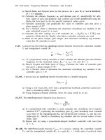
7;7. The imperfect mixing in a chemical reactor can be modeled by splitting the total volume
into two perfectly mixed sections with circulation between them. Feed enters and leaves
one section. The other section acts like a “side-capacity” element.
FIGURE P7.7

FIGURE P7.4
(‘11(\1’7‘t<K

7:
Laplace-Domain Dynamics
257
.
Assume holdups
and-
flow rates are constant. The reaction is an irreversible, tirst-
order consumption of reactant A. The system is isothermal. Solve for the transfer func-
tion relating C
~0
and
CA.
What are the
zeros
and poles of the transfer function? What
is the steady-state gain?
7.8. One way to determine the rate of change of a process variable is to measure the dif-
ferential pressure AP = P,,,
-
Pin
over a device called a derivative unit that has the
transfer function
Pout(.r)
7s

+

1
-

zz
Pin(.r)
(d6)s

+

1
(a) Derive the transfer function between AP and
Pi,.
(6) Show that the AP signal will be proportional to the rate of rise of
Pin,
after an initial
transient period, when Pi, is a ramp function.
Process p.
I”
Derivative
P
variable
___Jt__t
,I out
I,
-
signal
unit
L
L-c

-Ap
4
measurement
__ft__c
AP signal
A
FIGURE P7.8
7.9. A convenient way to measure the density of a liquid is to pump it slowly through a
vertical pipe and measure the differential pressure between the top and the bottom of
the pipe. This differential head is directly related to the density of the liquid in the pipe
if frictional pressure losses are negligible.
Suppose the density can change with time. What is the transfer function refating
a perturbation in density to the differential-pressure measurement? Assume the fluid
moves up the vertical column in plug flow at constant velocity.
Process fluid out
7-l
Process fluid in
Differential
-
with density
P(,)
pressure
//

-)
I,
AP signal
measurement
FIGURE P7.9
7.10. A thick-walled kettle of mass

MM,
temperature T
M,
and specific heat
CM
is filled \vith
a perfectly mixed process liquid of mass
M,
temperature T, and specific heat C. A
heating fluid at temperature
TJ
is circulated in a jacket around the kettle wall. The
heat transfer coefficient between the process fluid and the metal wall is
U
and between
the metal outside wall and the heating fluid is
U
,,,,.
Inside and outside heat transfer
258
i~~~rrwo:
Laplacc-Domain Dynamics and Control
areas A are approximately the same. Neglecting any radial temperature gradients
through the metal wall, show that the transfer function between T and TJ is two
first-order lags.
The value of the steady-state gain K,, is unity. Is this reasonable?
7.11. An ideal three-mode PID (proportional-integral-derivative) feedback controller is de-
scribed by the equation
CO,,, = Bias +
K,.

1
Derive the transfer function between
CO(s)
and
E(,Q.
Is this transfer function physically
realizable?
7.12. Show that the linearized nonisothermal CSTR of Example 7.6 can be stable only if
UA
vPc~

>
pC,RT2
-Ak

CAE

_

,$

_

k
7.13. A deadtime element is basically a distributed system. One approximate way to get
the dynamics of distributed systems is to lump them into a number of perfectly mixed
sections. Prove that a series of N mixed tanks is equivalent to a pure deadtime as N
goes to infinity. (Hint: Keep the total volume of the system constant as more and more
lumps are used.)
7.14. A feedback controller is added to the three-CSTR system of Example 7.5. Now

CAM
is
changed by the feedback controller to keep
CA3
at its setpoint, which is the steady-state
value of
CAJ.
The error signal is therefore just
-

CA3
(the perturbation in
C,Q).
Find the
transfer function of this closedloop system between the disturbance CA, and
CAM.
List
the values of poles, zeros, and steady-state gain when the feedback controller is:
(a) Proportional:
CAO
=
CAD
+
&(-C,43)
(b) Proportional-integral:
CA0
=
CAD
+
Kc

[-Cm
+
;/t-C,l)dr]
Note that these equations are in terms of perturbation variables,
7.15. The partial condenser sketched on the following page is described by two
ODES:
Vol dP
c-1
QC
RT dt
-=F-V-m
dMR

Qc
_
L
dt
=i?i
where P = pressure
Vol = volume of condenser
MR
= liquid holdup
F = vapor feed rate
V = vapor product
L = liquid product
CIIWIXK
7: Laplace-Domain Dynamics
259
L
FIGURE P7.15

(a) Draw a block diagram showing the transfer functions describing the
openloop
system.
(b)
Draw a block diagram of the closedloop system if a proportional controller is used
to manipulate
QC
to hold
MR
and a PI controller is used to manipulate V to hold P.
7.16. Show that a proportional-only level controller on a tank will give zero steady-state error
for a step change in level setpoint.
7.17. Use Laplace transforms to prove mathematically that a P controller produces steady-
state offset and that a PI controller does not. The disturbance is a step change in the
load variable. The process openloop transfer functions,
GM
and
GL,
are both first-order
lags with different gains but identical time constants.
7.18. Two loo-barrel tanks are available to use as surge volume to filter liquid flow rate
disturbances in a petroleum refinery. Average throughput is 14,400 barrels per day.
Should these tanks be piped up for parallel operation or for series operation? Assume
proportional-only level controllers.
7.19. A perfectly mixed batch reactor, containing 7500 lb, of liquid with a heat capacity of
1
Btu/lb,

OF,
is surrounded by a cooling jacket that is filled with 2480 lb, of perfectly

mixed cooling water.
At the beginning of the batch cycle, both the reactor liquid and the jacket ivater
are at 203°F. At this point in time, catalyst is added to the reactor and a reaction occurs
that generates heat at a constant rate of 15,300 Btu/min. At this same moment, makeup
cooling water at 68°F is fed into the jacket at a constant
832-lb,/min
flow rate.
The heat transfer area between the reactor and the jacket is 140
ft*.
The overall
heat transfer coefficient is 70 Btu/hr
“F

ft2.
Mass of the metal walls can be neglected.
Heat losses are negligible.
(a) Develop a mathematical model of the process.
(0) Use Laplace transforms to solve for the dynamic change in reactor temperature
%
260 I~~I‘Tw~: Lap/ace-Domain Dynamics anti Control
(c) What is the peak reactor temperature and when does it occur‘?
(n) What is the
final
steady-state reactor temperature?
7.20. The flow of air into the regenerator on a catalytic cracking unit is controlled by two
control valves. One is a large, slow-moving valve that is located on the suction of the
air blower. The other is a small, fast-acting valve that vents to the atmosphere.
The fail-safe condition is to not feed air into the regenerator. Therefore, the suction
valve is air-to-open and the vent valve is air-to-close. What action should the flow
controller have, direct or reverse?

The device with the following transfer function
Gcs)
is installed in the control line
to the vent valve.
7s
P
valve(s)
G(s) =
7s
=
~
CO(s)
The purpose of this device is to cause the vent valve to respond quickly to changes in
CO but to minimize the amount of air vented (since this wastes power) under steady-
state conditions. What will be the dynamic response of the perturbation in
P,,I,,
for a
step change of 10 percent of full scale in CO? What is the new steady-state value of
P
valve-
Atmospheric
Air to
suction
I
Vent
A
/;
/
/
,

co
// I,
I/ II II
cat. cracker
regenerator
FIGURE
P7.20
7.21. An openloop process has the transfer function
Calculate the openloop response of this process to a unit step change in its input. What
is the steady-state gain of this process?
7.22. A chemical reactor is cooled by both jacket cooling and autorefrigeration (boiling liq-
uid in the -reactor). Sketch a block diagram, using appropriate process and control
system transfer functions, describing the system. Assume these transfer functions are
known, either from fundamental mathematical models or from experimental dynamic
testing.
at
3-
01
re
ic
CHAPTER 7: Laplace-Domain Dynamics 261
Liquid
return
Cooling
jacket
Makeup
cooling
water
*
Discharge

25
pump
FIGURE P7.22
7.23. Solve the following problem, which is part of a problem given in Levenspiel’s Chem-
ical Reaction Engineering (1962, John Wiley, New York), using Laplace transform
techniques. Find analytical expressions for the number of Nelson’s ships
N(,)
and the
number of Villeneuve’s ships
Vo)
as functions of time.
The great naval battle, to be known to history as the battle of Trafalgar (1805), was
soon to be joined. Admiral Villeneuve proudly surveyed his powerful fleet of 33
ships stately sailing in single file in the light breeze. The British fleet under Lord
Nelson was now in sight, 27 ships strong. Estimating that it would still be two
hours before the battle, Villeneuve popped open another bottle of burgundy and
point by point reviewed his carefully thought out battle strategy. As was the custom
of naval battles at that time, the two fleets would sail in single file parallel to each
other and in the same direction, firing their cannons madly. Now, by long experi-
ence in battles of this kind, it was a well-known fact that the rate of destruction of a
fleet was proportional to the fire power of the opposing fleet. Considering his ships
to be on a par, one for one, with the British, Villeneuve was confident of victory.
Looking at his sundial, Villeneuve sighed and cursed the light wind; he’d never
get it over with in time for his favorite television western. “Oh’well,” he sighed,
“c’est
la vie.” He could see the headlines next morning. “British Fleet annihilated,
Villeneuve’s losses are. . .
.”
Villeneuve stopped short. How many ships would he
lose? Villeneuve called over his chief bottle cork popper, Monsieur Dubois. and

asked this question. What answer did he get?
7.24. While Admiral Villeneuve was doing his calculations about the outcome of the battle
of Trafalgar, Admiral Nelson was also doing some thinking. His fleet was outnumbered
33 to 27, so it didn’t take a rocket scientist to predict the outcome of the battle if the