Nonlinear controller design for active front steering system
Bạn đang xem bản rút gọn của tài liệu. Xem và tải ngay bản đầy đủ của tài liệu tại đây (939.99 KB, 6 trang )
Abstract— Active Front Steering system (AFS) provides an
electronically controlled superposition of an angle to the steering
wheel angle. This additional degree of freedom enables a continuous
and driving-situation dependent on adaptation of the steering
characteristics. In an active steering system, there needs be no fixed
relationship between the steering wheel and the angle of the road
wheels. Not only can the effective steering ratio be varied with speed,
for example, but also the road wheel angles can be controlled by a
combination of driver and computer inputs. Features like steering
comfort, effort and steering dynamics are optimized and stabilizing
steering interventions can be performed. In contrast to the
conventional stability control, the yaw rate was fed back to AFS
controller and the stability performance was optimized with Sliding
Mode control (SMC) method. In addition, tire uncertainties have
been taken into account in SM controller to provide the control
robustness. In this paper, 3-DOF nonlinear model is used to design
the AFS controller and 8-DOF nonlinear model is used to model the
controlled vehicle.
Keywords— Active Front Steering (AFS), Sliding Mode Control
method (SMC), Yaw rate, Vehicle Stability, Robustness
I. INTRODUCTION
CTIVE Front Steering ( AFS ) systems have been
introduced to improve handling stability under adverse
road conditions. The law in some countries requires that
there must be a direct mechanical connection between the
driver's steering wheel and the road wheels. This would seem
to make an active steering drive-by-wire system impossible.
This is not quite the case, however. If a differential element is
inserted in the steering column, then the steer angle of the road
wheels can be the sum of two angular inputs. One can be the
steer angle commanded by the driver through the steering
wheel and the other can be the angle from a rotary actuator,
such as an electric motor and gear train, commanded by a
computer. In an active steering system, there needs be no fixed
relationship between the steering wheel angle and the angle of
the road wheels. This means that the response of the steering
wheel inputs can be varied and an automobile can be made to
I.Mousavinejad is graduate student ( M.sc degree) in Sharif University of
Technology –International campus-Kish island , Iran,
Tel:22299665 (+9821)
Email :
R.Kazemi is associate professor in mechanical engineering faculty of
K.N.Toosi University of Technology. No.15, Pardis St, Mollasadra Ave,
Vanak Sq, Tehran, Iran. P.o.Box : 19395-1999, Tel:88674747 (+9821),
Fax:88674748 (+9821) , Email :
M.Bayani is graduate student (M.sc degree) in K.N.Toosi University of
Technology. No.15, Pardis St., Mollasadra Ave, Vanak Sq, Tehran, Iran.
P.o.Box : 19395-1999, Email :
respond to steering inputs much as a reference vehicle would.
[1, 2]
At slow speed, the steering is made more responsive so
less motion of the steering wheel is required for parking but at
high speeds the steering ratio is made slower so that the driver
does not feel that the car reacts too violently.
Huh and Kim (2001) devise an active steering controller
that eliminates the difference in steering response between
driving on slippery roads and dry roads. The controller is
based on feedback of lateral tire force estimates derived from
vehicle roll motion. [3]
Segawa et al (2002) apply lateral acceleration and yaw rate
feedback to a steer-by-wire vehicle and demonstrate that
active steering control can achieve greater driving stability
than differential brake control. [4]
W.Klier et al (2003) proposed the concept and
functionality of the active front steering system. They focused
on a modular system concept and its respective advantages
and requirements. [5]
D.Chen et al (2008) proposed the controller for an active
front steering system. In this research the stability
performance has been optimized with LQR (Linear Quadratic
Regulator). HILS (Hardware-In-the-Loop Simulation) tests
were conducted to demonstrate the performance of the
designed AFS controller. [1]
This paper discusses a yaw stability control algorithm. The
controller is designed based on the sliding mode method to
improve the vehicle stability and maneuverability.
II. VEHICLE MODELING
In this paper three-degree-freedom (3-DOF) model will be
utilized for the AFS controller design and eight-degree-
freedom (8-DOF) model will be used as a controlled plant of
the vehicle for control system evaluations through computer
simulations.
A. 8-DOF Vehicle Model
A nonlinear vehicle handling model which is used for
simulation purpose is developed for this study. The vehicle is
modeled based on this model to be controlled by the AFS
controller. This model consists of 8-DOF which include three
planar motions of the vehicle plus body roll motion relative to
the chassis about the roll axis and the rotational dynamics of
four wheels. Fig.1 shows the vehicle model with coordinate
system, degrees of freedom and external forces. The equations
of motion for the model are given as:
Longitudinal motion:
݉
൫
ܸ
ሶ
௫
െ ݎܸ
௬
൯
െ ݉
௦
݄
ሺ
߮ݎሶെ 2ݎሶ߮
ሻ
ൌ
∑
ܨ
௫
(1)
Nonlinear Controller Design for Active Front
Steering System
Iman Mousavinejad, Reza Kazemi, and Mohsen Bayani Khaknejad
A
World Academy of Science, Engineering and Technology
International Journal of Mechanical, Industrial Science and Engineering Vol:6 No:1, 2012
6
International Science Index Vol:6, No:1, 2012 waset.org/Publication/9997443
Lateral motion:
݉
൫
ܸ
ሶ
௬
ܸ
௫
ݎ
൯
݉
௦
݄
ሺ
߮ሷെ ݎ
ଶ
߮
ሻ
ൌ
∑
ܨ
௬
(2)
Yaw motion:
ܫ
௭௭
ݎሶ
ሺ
ܫ
௭௭
ߛ െ ܫ
௫௭
߮ሷ
ሻ
െ ݉
௦
݄
൫
ܸ
ሶ
௫
െ ݎܸ
௬
൯
߮ൌ
∑
ܯ
௭
(3)
Roll motion:
ሺ
ܫ
௫௫
݄݉
ଶ
ሻ
߮ሷ ݉
௦
݄
൫
ܸ
ሶ
௬
ܸ
௫
ݎ
൯
ሺ
ܫ
௭௭
ߛ െܫ
௫௭
ሻ
ݎሶെ
൫
݄݉
ଶ
ܫ
௬௬
െ ܫ
௭௭
൯
ݎ
ଶ
߮ൌ
∑
ܯ
௫
(4)
Wheel motion:
ܫ
௪
߱ሶ
ൌെܴ
௪
ܨ
௫௪
ܶ
(5)
Where:
∑
ܨ
௫
ൌܨ
௫ଵ
ܨ
௫ଶ
ܨ
௫ଷ
ܨ
௫ସ
(6)
∑
ܨ
௬
ൌܨ
௬ଵ
ܨ
௬ଶ
ܨ
௬ଷ
ܨ
௬ସ
(7)
∑
ܯ
௭
ൌ݈
൫ܨ
௬ଵ
ܨ
௬ଶ
൯ െ ݈
൫ܨ
௬ଷ
ܨ
௬ସ
൯ ܯ
௭
(8)
∑
ܯ
௫
ൌൣ݉
௦
݄݃ െ ൫ܭ
ఝ
ܭ
ఝ
൯൧߮ െ ൫ܥ
ఝ
ܥ
ఝ
൯߮ሶ (9)
݉ൌ ݉
௦
݉
௨
݉
௨
(10)
ܯ
௭
ൌ
௧
ଶ
ሾሺ
ܨ
௫ଵ
ܨ
௫ଷ
ሻ
െ
ሺ
ܨ
௫ଶ
ܨ
௫ସ
ሻሿ
(11)
Fig.1 8-DOF vehicle model [7]
In the above equations, the resultant longitudinal and
lateral forces acting on the ith wheel in the vehicle fixed
coordinate system, F
xi
and F
yi
, have the following relationships
with the tire forces along the wheel axes, F
xwi
and F
ywi
, as
shown in Fig.2.
Fig.2 Wheel definition [7]
൜
ܨ
௫
ܨ
௬
ൠൌ
cosߜ
െsinߜ
sinߜ
cosߜ
൨൜
ܨ
௫௪
ܨ
௬௪
ൠ
ሺ
݅ൌ1,…,4
ሻ
(12)
Because of the suspension system is not considered in this
modeling and normal tire forces have an effect on the
longitudinal, lateral forces and the self-aligning torque, the
normal forces should be modeled as following equations.
According to the quasi-static longitudinal and lateral load
transfers, the instantaneous vertical tire load acting on each
wheel F
zi
during dynamic maneuvers is the sum of the static
tire load plus transfer that is due to longitudinal acceleration,
lateral acceleration, and body roll motion respectively. This
effect can be described as:
ܨ
௭ଵ
ൌ
ೝ
ଶ
െ
ೣ
ଶ
௧
ቀ
ೞ
ೝೞ
݉
௨
݄
௨
ቁ
ଵ
௧
൫െܭ
ఝ
߮ െ ܥ
ఝ
߮ሶ൯ (13)
ܨ
௭ଶ
ൌ
ೝ
ଶ
െ
ೣ
ଶ
െ
௧
ቀ
ೞ
ೝೞ
݉
௨
݄
௨
ቁ
െ
ଵ
௧
൫െܭ
ఝ
߮ െܥ
ఝ
߮ሶ൯ (14)
ܨ
௭ଷ
ൌ
ଶ
ೣ
ଶ
௧
ቀ
ೞ
ೞ
ೝ
݉
௨
݄
௨
ቁ
ଵ
௧
൫െܭ
ఝ
߮ െ ܥ
ఝ
߮ሶ൯ (15)
ܨ
௭ସ
ൌ
ଶ
ೣ
ଶ
െ
௧
ቀ
ೞ
ೞ
ೝ
݉
௨
݄
௨
ቁ
െ
ଵ
௧
൫െܭ
ఝ
߮ െ ܥ
ఝ
߮ሶ൯ (16)
B. 3-DOF Vehicle Model
The three degrees of freedom (3-DOF) model, which is a
good representation of the lateral vehicle dynamics in the
nonlinear handling region, is employed for AFS controller
design. The states in this model are Lateral motion, yaw
motion and roll motion. This model can be described by the
following state equations with small wheel angle and constant
forward speed assumptions:
ܸ
ሶ
௬
ൌെݎܸ
௫
െ ݄߮ሷ݄ݎ
ଶ
߮
ଵ
൫ܨ
௬
ܨ
௬
൯ (17)
ݎሶൌ
ଵ
ூ
ൣ
ሺ
ܫ
௭௭
ߛ െܫ
௫௭
ሻ
ሷ
݄݉൫െݎܸ
௬
൯ ܨ
௬
ܮ
െ
ܨ
௬
ܮ
൧
ሺ18ሻ
߮ሷൌ
ଵ
ሺ
ூ
ೣೣ
ା
మ
ሻ
ൣെ݄݉ ൫ܸ
ሶ
௬
ݎܸ
௫
൯
ሺ
ܫ
௭௭
ߛെ ܫ
௫௭
ሻ
ݎሶ
൫݄݉
ଶ
ܫ
௬௬
െ ܫ
௭௭
൯ݎ
ଶ
߮ െ൫ܥ
ఝ
ܥ
ఝ
൯߮ሶെ
൫ܭ
ఝ
ܭ
ఝ
െ ݄݉݃൯߮
൧
(19)
In this model ܨ
௬
and ܨ
௬
is computed based on the linear tire
model.
III. TIRE MODELING
In order to simulate the limit handling situations where
strong non-linearity is present, the nonlinear ' PACEJKA' tire
model [6] with combined longitudinal and lateral slip is
employed the tire forces can be illustratively express as:
World Academy of Science, Engineering and Technology
International Journal of Mechanical, Industrial Science and Engineering Vol:6 No:1, 2012
7
International Science Index Vol:6, No:1, 2012 waset.org/Publication/9997443
൛
ܨ
௫௪
,ܨ
௬௪
ൟ
ൌ݂
ሺ
ߣ
,ߙ
,ܨ
௭
ሻ
(20)
In recent years, an empirical method for characterizing tire
behavior known as the Magic Formula has been developed
and used in vehicle handling simulations. The Magic Formula,
in its basic form, can be used to fit experimental tire data for
characterizing the relationships between the cornering force
and slip angle, self-aligning torque and slip angle, or braking
effort and skid. It is expressed by:
ݕ
ሺ
ݔ
ሻ
ൌܦ sin
ሼ
ܥ tan
ିଵ
ሾ
ܤݔെ ܧ
ሺ
ܤݔെ tan
ିଵ
ܤݔ
ሻሿሽ
(21)
ܻ
ሺ
ܺ
ሻ
ൌݕ
ሺ
ݔ
ሻ
ܵ
௩
ݔൌܺ ܵ
Where Y(X) represents cornering force, self-aligning
torque, or braking effort and X denotes slip angle or skid.
Coefficient B is called stiffness factor, C shape factor, D peak
factor, and E curvature factor .S
h
and S
v
are the horizontal
shift and vertical shift, respectively. (For further information
refer to Ref [6])
The linear tire model equation is used to design the AFS
controller but the 'PACEJKA' tire model is used to model the
controlled plant of the vehicle.
ܨ
௬
ൌ2ܥ
ఈ
ߙ
ሺ22ሻ
IV. AFS CONTROLLER DESIGN
In this paper the AFS controller is designed based on the
Sliding Mode Control (SMC) method to improve vehicle
steerability by tracking the reference yaw rate. The reference
model of this controller is based on the 3-DOF vehicle model.
Model imprecision may come from actual uncertainty about
the plant (e.g., unknown plant parameters), or from the
purposeful choice of a simplified representation of the system's
dynamics (e.g., modeling friction as linear, or neglecting
structural modes in a reasonably rigid mechanical system).
From a control point of view, modeling inaccuracies can be
classified into two major kinds [8]:
• Structured (or parametric) uncertainties
• Unstructured uncertainties (or un-modeled dynamics)
It is believed that drivers intend to control the yaw rate
when the vehicle travels around a corner; therefore the
reference model indeed reflects the desired relationship
between the driver steer inputs and the vehicle yaw rate. The
yaw rate generated by the reference model is therefore chosen
as the reference signal to be tracked by the active front
steering controller. Consequently, the AFS controller is
designed to force the vehicle to follow the reference yaw rate
through driving the tracking error between the actual and
desired yaw to zero. In this way, they make contributions to
steerability improvement by assisting the driver in steering the
vehicle and helping the driver to avoid extreme handling
situations. The AFS acts as a steering correction system by
applying an additional steer angle to that demanded by the
driver.
ߜൌߜ
ߜ
(23)
The driver's input is:
ߜ
ൌ
ఋ
ೞ
ைௌோ
(24)
The OSR term is Overall Steering Ratio that is 17.4 in a
conventional vehicle. Now by following equations, the AFS
controller is designed based on the Sliding Mode Control
method.
݁ൌݎെݎ
ௗ
ݐ݄݁ ݁ݎݎݎ (25)
݁ሶൌݎሶെ ݎሶ
ௗ
(26)
The following sliding surface and sliding reachability
condition are selected.
ݏൌ݁ (27)
ݏሶൌെߣݏ ՜ ݁ሶൌെߣ݁ ՜ ݁ሶ ߣ݁ൌ0
(28)
Now, the 3-DOF vehicle model equations (17-19) and
equations (27 & 28) are used to derive the sliding control low:
ሺ
ଵ଼
ሻ
,ሺଶሻ
ሱ
ۛ
ۛ
ۛ
ۛ
ۛ
ۛ
ሮ
݁ሶൌݎሶെ ݎሶ
ௗ
ൌ
1
ܫ
௭௭
ൣ
ሺ
ܫ
௭௭
ߛെ ܫ
௫௭
ሻ
ሷ
݄݉൫െݎܸ
௬
൯
ܨ
௬
ܮ
െ ܨ
௬
ܮ
൧
െ ݎሶ
ௗ
ሺ29ሻ
ሺ
ଶହ
ሻ
,
ሺ
ଶ଼
ሻ
,ሺଶଽሻ
ሱ
ۛ
ۛ
ۛ
ۛ
ۛ
ۛ
ۛ
ۛ
ۛ
ۛ
ሮ
ଵ
ூ
ሺ
ܫ
௫௭
െ ܫ
௭௭
ߛ
ሻ
ሷ
݄݉൫െݎܸ
௬
൯
2ܮ
ܥ
ఈ
ߜ
െ
ቀ
ଶ
ഀ
ିଶ
ೝ
ഀೝ
ೣ
ቁ
ܸ
௬
െ
൬
ଶ
మ
ഀ
ାଶ
ೝ
మ
ഀೝ
ೣ
൰
ݎ
൨
െ ݎሶ
ௗ
ߣ
ሺ
ݎെ ݎ
ௗ
ሻ
ൌ0
(30)
ߜ
ൌ
1
2݈
ܥ
ఈ
ቌ
ݎሶ
ௗ
െ
1
ܫ
௭௭
ቈ
ሺ
ܫ
௫௭
െ ܫ
௭௭
ߛ
ሻ
ሷ
݄݉൫െݎܸ
௬
൯
െ ൬
2ܮ
ܥ
ఈ
െ 2ܮ
ܥ
ఈ
ܸ
௫
൰ܸ
௬
െ ቆ
2ܮ
ଶ
ܥ
ఈ
2ܮ
ଶ
ܥ
ఈ
ܸ
௫
ቇݎ
ߣ
ሺ
ݎ
ௗ
െ ݎ
ሻ
൱
ሺ31ሻ
ߜൌߜ
െ ݇כ ݏ݃݊
ሺ
ݏ
ሻ
՜
ߜൌߜ
െ ݇כ ݏ݃݊
ሺ
ݎ െݎ
ௗ
ሻ
(32)
Where λ and k are positive parameters to be tuned in controller
design and sgn() is the sign function.
However, the presence of the discontinuous term in equation
(32) may cause chattering, which involves extremely high
control effort and may also excite high-frequency unmodeled
dynamics [8]. In order to eliminate this effect, the sign
World Academy of Science, Engineering and Technology
International Journal of Mechanical, Industrial Science and Engineering Vol:6 No:1, 2012
8
International Science Index Vol:6, No:1, 2012 waset.org/Publication/9997443
function in equation (32) is replaced by the saturation
function,ݏܽݐሺݏ
⁄
ሻ, which is used to approximate a continuous
control within a boundary layer around the sliding surface.
The saturation function ݏܽݐሺݏ
⁄
ሻ is defined as:
ݏܽݐ
ሺ
ݏ
⁄ ሻ
ൌ൜
ݏ
⁄
݂݅
|
ݏ
|
ݏ݃݊
ሺ
ݏ
⁄ ሻ
݂݅
|
ݏ
|
(33)
Thus the continuous approximation of the control law in
equation (32) is given as:
ߜൌߜ
െ ݇כ ݏܽݐ
ቀ
ି
థ
ቁ
(34)
Where is the boundary layer thickness.
Where r
d
is desired yaw rate in under-steer condition.
ݎ
ௗ
ൌ
ೣ
ఋ
൫ ଵା
ೠ
ೣ
మ
൯
(35)
Where L = L
f
+ L
r
and K
u
is the under-steer coefficient and
calculated by following equation:
ܭ
௨
ൌ
൫
ೝ
ഀೝ
ି
ഀ
൯
ଶ
ഀ
ഀೝ
మ
(36)
Fig.3 AFS controller block diagram
V. RESULTS
In the processes of design, development and improvement
of the vehicle, first the vehicle is evaluated with the simulation
software on the computer before the designed system or
subsystem is evaluated on a real vehicle and proving ground.
MATLAB software is used for the simulation.
To evaluate the performance of the AFS controller, the
slalom maneuver is used (Fig.4). In this maneuver the
sinusoidal torque is exerted on the steering wheel by the
driver. The friction coefficient between the tire and the road
surface is 0.8, therefore the vehicle is moving on a dry road.
The initial speed of the vehicle is about 80 Km/h. This
maneuver is used to evaluate the speed of the performance and
the response of the controlling system when it encounters
disturbances.
Fig.6 shows the angle of the front wheels where δ
f
is the
conventional angle and δ
f
+ δ
c
is the angle, which is corrected
by the AFS controller. Fig.7 shows the corrective angle, which
is added to the driver's input by the AFS controller.
The deviation of the conventional vehicle from the desired
track of the vehicle is larger than that of the controlled vehicle
as shown in Fig.8.
As shown in Fig.9, the uncontrolled vehicle behaves badly
with respect to the deriver's input while the controlled vehicle
covers the desired yaw rate properly. Fig.10 demonstrates the
high capability of the controller to control the lateral speed of
the vehicle.
Fig.4 Driver's torque
Fig.5 Steering wheel angle
Fig.6 Front wheel angle
Fig.7 AFS corrective angle
Fig.8 Vehicle track
World Academy of Science, Engineering and Technology
International Journal of Mechanical, Industrial Science and Engineering Vol:6 No:1, 2012
9
International Science Index Vol:6, No:1, 2012 waset.org/Publication/9997443
Fig.9 Vehicle yaw rate
Fig.10 Lateral speed of the vehicle's center of gravity
Fig.11 Lateral acceleration of the vehicle
Fig.12 AFS controller error
VI. CONCLUSION
In this paper, a new method for the vehicle dynamics
control was described. For this reason, the sliding mode
controller has been used to design the active front steering
controller.
• The 8-DOF model has been provided to simulate the
vehicle and the assessment of the function of vehicle
stability control systems.
• The PACEJKA tire model with combined longitudinal and
lateral slip has been used to model the tire's nonlinear
characteristics.
• The yaw stability controller as the Active Front Steering
System (AFS) has been designed based on the sliding
mode control method and 3-DOF nonlinear model. This
controller corrects the angle of the front wheels to control
the yaw rate of the vehicle. Therefore this controller
improves the stability and maneuverability of the vehicle
on dry roads, wet roads and snowy roads.
At the end, in order for the present research to be more
complete and practical, the following future works are
proposed:
• The evaluation of the differential braking system and anti-
lock brake system's performance when the active front
steering system is used in the vehicle.
• The simulation of the driver and the evaluation of the
driver's role in the dynamics behavior of the vehicle which
is equipped with these controllers.
• The usage of the other methods to design the controllers
and compare these systems to other controlling systems.
• Design estimators and observers to estimate the mass,
moment of inertia of the vehicle and the longitudinal and
lateral forces of the tire, and evaluate the effects of these
elements on the performance of the controllers.
APPENDIX
TABLE I
VALUE OF PARAMETERS [7]
Variable name
Variable magnitude
Variable unit
m
1300
Kg
m
s
1095.7 Kg
m
uf
95.5 Kg
m
ur
108.8 Kg
L
fs
1.2227 m
L
rs
1.4393 m
L
f
1.2247 m
L
r
1.4373 m
t 1.4376 m
h
cg
0.5253 m
h
uf
0.313 m
h
ur
0.313 m
h
0.445 m
h
f
0.130 m
h
r
0.110 m
I
xx
346.7 Kg-m
2
I
zz
1808.8 Kg-m
2
I
xz
21.09 Kg-m
2
I
w
2.11 Kg-m
2
R
w
0.285 m
K
φf
66175 N-m/rad
K
φr
66175 N-m/rad
C
φf
3511 N-m-s/rad
C
φr
3511 N-m-s/rad
g
9.81 m/s
2
γ
0.854 deg
C
αf
60000 N/rad
C
αr
60000 N/rad
World Academy of Science, Engineering and Technology
International Journal of Mechanical, Industrial Science and Engineering Vol:6 No:1, 2012
10
International Science Index Vol:6, No:1, 2012 waset.org/Publication/9997443
TABLE 2
DEFINITION OF PARAMETERS [7]
Notation Description unit
C
αf
, C
αr
Cornering Stiffness of
Front , rear axle
N/rad
C
φf
, C
φr
Front , rear suspension
roll damping
Nm/rad s
h Distance from sprung
mass centre of gravity
(CG) to the roll axis
m
h
cg
Height of vehicle CG m
h
f
, h
r
Height of front , rear
roll centre
m
h
uf
, h
ur
Height of front , rear
unsprung mass CG
m
I
w
Wheel moment of
inertia about the spin
axis
Kg m
2
I
xx
Sprung mass moment
of inertia about the roll
axis
Kg m
2
I
xz
Sprung mass product
of inertia about the roll
and yaw axes
Kg m
2
I
zz
Vehicle moment of
inertia about the z axis
Kg m
2
K
φf
, K
φr
Front , rear suspension
roll stiffness
N m /rad
L
f
, L
r
Distance from the
vehicle CG to the front
, rear axle
m
L
fs
, L
rs
Distance from the
sprung mass CG to the
front , rear axle
m
m
uf
, m
ur
Front , rear un-sprung
mass
Kg
m , m
s
Total mass , sprung
mass of the vehicle
Kg
t Wheel track m
R
w
Effective wheel rolling
Radius
m
γ Inclined angle between
roll axis and x axis
deg
V
x
, V
y
Longitudinal , lateral
speed of the vehicle's
center of gravity
m/s
a
x
, a
y
Longitudinal , lateral
acceleration of the
vehicle's body
m/s
2
ϕ
roll angle rad
r Yaw rate rad/s
λ
i
Longitudinal slip -
α Lateral slip rad
F
x
, F
y
, F
z
Longitudinal , Lateral ,
Normal force of tire
N
REFERENCES
[1] D.Chen, C.Yin and J.Zhang, "Controller design of a new active front
steering system," WSEAS Transaction on systems, 2008, issue 11,vol.7,
pp1258-1268.
[2] D.Karnopp, Vehicle Stability. Marcel Dekker, 2004.
[3] K.Huh and J.Kim, "Active steering control based on the estimated tire
forces," Journal of Dynamic Systems, Measurement, and Control, vol.123,
pp.505-511, 2001.
[4] M.Segawa, K.Nishizaki and S.Nakano, "A Study of vehicle stability
control by steer by wire system," Proceedings of the International
Symposium on Advanced Vehicle control (AVEC), Ann Arbor, MI, 2002.
[5] W.Klier, G.Reimann and W.Reinelt, "Concept and Functionality of the
active front steering system," SAE International Conf, 2004-21-0073.
[6] H.B.Pacejka , Tire and Vehicle Dynamics , Delf university of technology.
[7] I.Mousavinejad, Nonlinear Controller Design for Steer-By-Wire Passenger
Car. Master Thesis, Sharif University of Technology, 2009.
[8] Slotine.Li , Applied Nonlinear Control. Prentice Hall, 1991.
World Academy of Science, Engineering and Technology
International Journal of Mechanical, Industrial Science and Engineering Vol:6 No:1, 2012
11
International Science Index Vol:6, No:1, 2012 waset.org/Publication/9997443