Giáo trình robot - Phần 3 pptx
Bạn đang xem bản rút gọn của tài liệu. Xem và tải ngay bản đầy đủ của tài liệu tại đây (880.33 KB, 85 trang )
Part II
Position Control
Introduction to Part II
Depending on their application, industrial robot manipulators may be classi-
fied into two categories: the first is that of robots which move freely in their
workspace (i.e. the physical space reachable by the end-effector) thereby un-
dergoing movements without physical contact with their environment; tasks
such as spray-painting, laser-cutting and welding may be performed by this
type of manipulator. The second category encompasses robots which are de-
signed to interact with their environment, for instance, by applying a comply-
ing force; tasks in this category include polishing and precision assembling.
In this textbook we study exclusively motion controllers for robot manip-
ulators that move about freely in their workspace.
For clarity of exposition, we shall consider robot manipulators provided
with ideal actuators, that is, actuators with negligible dynamics or in other
words, that deliver torques and forces which are proportional to their inputs.
This idealization is common in many theoretical works on robot control as well
as in most textbooks on robotics. On the other hand, the recent technological
developments in the construction of electromechanical actuators allow one to
rely on direct-drive servomotors, which may be considered as ideal torque
sources over a wide range of operating points. Finally, it is important to
mention that even though in this textbook we assume that the actuators are
ideal, most studies of controllers that we present in the sequel may be easily
extended, by carrying out minor modifications, to the case of linear actuators
of the second order; such is the case of DC motors.
Motion controllers that we study are classified into two main parts based on
the control goal. In this second part of the book we study position controllers
(set-point controllers) and in Part III we study motion controllers (tracking
controllers).
Consider the dynamic model of a robot manipulator with n DOF, rigid
links, no friction at the joints and with ideal actuators, (3.18), and which we
recall below for convenience:
136 Part II
M(q)
¨
q + C(q,
˙
q)
˙
q + g(q)=τ . (II.1)
where M (q) ∈ IR
n×n
is the inertia matrix, C(q,
˙
q)
˙
q ∈ IR
n
is the vector of
centrifugal and Coriolis forces, g(q) ∈ IR
n
is the vector of gravitational forces
and torques and τ ∈ IR
n
is a vector of external forces and torques applied
at the joints. The vectors q,
˙
q,
¨
q ∈ IR
n
denote the position, velocity and joint
acceleration respectively.
In terms of the state vector
q
T
˙
q
T
T
these equations take the form
d
dt
⎡
⎣
q
˙
q
⎤
⎦
=
⎡
⎣
˙
q
M(q)
−1
[τ (t) −C(q,
˙
q)
˙
q − g(q)]
⎤
⎦
.
The problem of position control of robot manipulators may be formulated
in the following terms. Consider the dynamic equation of an n-DOF robot,
(II.1). Given a desired constant position (set-point reference) q
d
, we wish to
find a vectorial function τ such that the positions q associated with the robot’s
joint coordinates tend to q
d
accurately.
In more formal terms, the objective of position control consists in finding
τ such that
lim
t→∞
q(t)=q
d
where q
d
∈ IR
n
is a given constant vector which represents the desired joint
positions.
The way that we evaluate whether a controller achieves the control ob-
jective is by studying the asymptotic stability of the origin of the closed-loop
system in the sense of Lyapunov (cf. Chapter 2). For such purposes, it appears
convenient to rewrite the position control objective as
lim
t→∞
˜
q(t)=0
where
˜
q ∈ IR
n
stands for the joint position errors vector or is simply called
position error, and is defined by
˜
q(t):=q
d
− q(t) .
Then, we say that the control objective is achieved, if for instance the
origin of the closed-loop system (also referred to as position error dynamics)
in terms of the state, i.e. [
˜
q
T
˙
q
T
]
T
= 0 ∈ IR
2n
, is asymptotically stable.
The computation of the vector τ involves, in general, a vectorial nonlinear
function of q,
˙
q and
¨
q. This function is called the “control law” or simply,
“controller”. It is important to recall that robot manipulators are equipped
with sensors to measure position and velocity at each joint, hence, the vectors
q and
˙
q are assumed to be measurable and may be used by the controllers.
In general, a control law may be expressed as
Introduction to Part II 137
τ = τ (q,
˙
q,
¨
q, q
d
,M(q),C(q,
˙
q), g(q)) . (II.2)
However, for practical purposes it is desirable that the controller does not
depend on the joint acceleration
¨
q, because measurement of acceleration is
unusual and accelerometers are typically highly sensitive to noise.
Figure II.1 presents the block-diagram of a robot in closed loop with a
position controller.
ROBOT
CONTROLLER
τ
q
˙
q
q
d
Figure II.1. Position control: closed-loop system
If the controller (II.2) does not depend explicitly on M(q), C(q,
˙
q) and
g(q), it is said that the controller is not “model-based”. This terminology is,
however, a little misfortunate since there exist controllers, for example of the
PID type (cf. Chapter 9), whose design parameters are computed as functions
of the model of the particular robot for which the controller is designed. From
this viewpoint, these controllers are model-dependent or model-based.
In this second part of the textbook we carry out stability analyses of
a group of position controllers for robot manipulators. The methodology to
analyze the stability may be summarized in the following steps.
1. Derivation of the closed-loop dynamic equation. This equation is obtained
by replacing the control action τ (cf. Equation II.2 ) in the dynamic model
of the manipulator (cf. Equation II.1). In general, the closed-loop equation
is a nonautonomous nonlinear ordinary differential equation.
2. Representation of the closed-loop equation in the state-space form, i.e.
d
dt
q
d
− q
˙
q
= f(q,
˙
q, q
d
,M(q),C(q,
˙
q), g(q)) . (II.3)
This closed-loop equation may be regarded as a dynamic system whose
inputs are q
d
,
˙
q
d
and
¨
q
d
, and with outputs, the state vectors
˜
q = q
d
− q
and
˙
q. Figure II.2 shows the corresponding block-diagram.
3. Study of the existence and possible unicity of equilibrium for the closed-
loop equation. For this, we rewrite the closed-loop equation (II.3) in the
state-space form choosing as the state, the position error and the velocity.
138 Part II
CONTROLLER
ROBOT
+
q
d
˜
q
˙
q
Figure II.2. Set-point control closed-loop system. Input–output representation.
That is, let
˜
q := q
d
−q denote the state of the closed-loop equation. Then,
(II.3) becomes
d
dt
˜
q
˙
q
=
˜
f(
˜
q,
˙
q) (II.4)
where
˜
f is obtained by replacing q with q
d
−
˜
q. Note that the closed-loop
system equation is autonomous since q
d
is constant.
Thus, for Equation (II.4) we want to verify that the origin, [
˜
q
T
˙
q
T
]
T
=
0 ∈ IR
2n
is an equilibrium and whether it is unique.
4. Proposal of a Lyapunov function candidate to study the stability of the
origin for the closed-loop equation, by using the Theorems 2.2, 2.3, 2.4
and 2.7. In particular, verification of the required properties, i.e. positivity
and negativity of the time derivative.
5. Alternatively to step 4, in the case that the proposed Lyapunov function
candidate appears to be inappropriate (that is, if it does not satisfy all of
the required conditions) to establish the stability properties of the equilib-
rium under study, we may use Lemma 2.2 by proposing a positive definite
function whose characteristics allow one to determine the qualitative be-
havior of the solutions of the closed-loop equation.
It is important to underline that if Theorems 2.2, 2.3, 2.4, 2.7 and Lemma
2.2 do not apply because one of their conditions does not hold, it does not
mean that the control objective cannot be achieved with the controller under
analysis but that the latter is inconclusive. In this case, one should look for
other possible Lyapunov function candidates such that one of these results
holds.
The rest of this second part of the textbook is divided into four chapters.
The controllers that we present may be called “conventional” since they are
commonly used in industrial robots. These controllers are:
• Proportional control plus velocity feedback and Proportional Derivative
(PD) control;
• PD control with gravity compensation;
Bibliography 139
• PD control with desired gravity compensation;
• Proportional Integral Derivative (PID) control.
Bibliography
Among books on robotics, robot dynamics and control that include the study
of tracking control systems we mention the following:
• Paul R., 1982, “Robot manipulators: Mathematics programming and con-
trol”, MIT Press, Cambridge, MA.
• Asada H., Slotine J. J., 1986, “Robot analysis and control ”, Wiley, New
York.
• Fu K., Gonzalez R., Lee C., 1987, “Robotics: Control, sensing, vision and
intelligence”, McGraw–Hill.
• Craig J., 1989, “Introduction to robotics: Mechanics and control”, Addison-
Wesley, Reading, MA.
• Spong M., Vidyasagar M., 1989, “Robot dynamics and control”, Wiley,
New York.
• Yoshikawa T., 1990, “Foundations of robotics: Analysis and control”, The
MIT Press.
• Spong M., Lewis F. L., Abdallah C. T., 1993, “Robot control: Dynamics,
motion planning and analysis”, IEEE Press, New York.
• Sciavicco L., Siciliano B., 2000, “Modeling and control of robot manipula-
tors”, Second Edition, Springer-Verlag, London.
Textbooks addressed to graduate students are (Sciavicco and Siciliano,
2000) and
• Lewis F. L., Abdallah C. T., Dawson D. M., 1993, “Control of robot ma-
nipulators”, Macmillan Pub. Co.
• Qu Z., Dawson D. M., 1996, “Robust tracking control of robot manipula-
tors”, IEEE Press, New York.
• Arimoto S., 1996, “Control theory of non–linear mechanical systems”, Ox-
ford University Press, New York.
More advanced monographs addressed to researchers and texts for gradu-
ate students are
• Ortega R., Lor´ıa A., Nicklasson P. J., Sira-Ram´ırez H., 1998, “Passivity-
based control of Euler-Lagrange Systems Mechanical, Electrical and Elec-
tromechanical Applications”, Springer-Verlag: London, Communications
and Control Engg. Series.
140 Part II
• Canudas C., Siciliano B., Bastin G. (Eds), 1996, “Theory of robot control”,
Springer-Verlag: London.
• de Queiroz M., Dawson D. M., Nagarkatti S. P., Zhang F., 2000, “Lyapunov–
based control of mechanical systems”, Birkh¨auser, Boston, MA.
A particularly relevant work on robot motion control and which covers in
a unified manner most of the controllers that are studied in this part of the
text, is
• Wen J. T., 1990, “A unified perspective on robot control: The energy
Lyapunov function approach”, International Journal of Adaptive Control
and Signal Processing, Vol. 4, pp. 487–500.
6
Proportional Control plus Velocity Feedback
and PD Control
Proportional control plus velocity feedback is the simplest closed-loop con-
troller that may be used to control robot manipulators. The conceptual ap-
plication of this control strategy is common in angular position control of DC
motors. In this application, the controller is also known as proportional control
with tachometric feedback. The equation of proportional control plus velocity
feedback is given by
τ = K
p
˜
q − K
v
˙
q (6.1)
where K
p
,K
v
∈ IR
n×n
are symmetric positive definite matrices preselected by
the practitioner engineer and are commonly referred to as position gain and
velocity (or derivative) gain, respectively. The vector q
d
∈ IR
n
corresponds to
the desired joint position, and the vector
˜
q = q
d
− q ∈ IR
n
is called position
error. Figure 6.1 presents a block-diagram corresponding to the control system
formed by the robot under proportional control plus velocity feedback.
˙
q
q
ROBOTq
d
ΣΣ
K
p
K
v
τ
Figure 6.1. Block-diagram: Proportional control plus velocity feedback
Proportional Derivative (PD) control is an immediate extension of propor-
tional control plus velocity feedback (6.1). As its name suggests, the control
law is not only composed of a proportional term of the position error as in the
case of proportional control, but also of another term which is proportional
to the derivative of the position, i.e. to its velocity error,
˙
˜
q. The PD control
142 6 Proportional Control plus Velocity Feedback and PD Control
law is given by
τ = K
p
˜
q + K
v
˙
˜
q (6.2)
where K
p
,K
v
∈ IR
n×n
are also symmetric positive definite and selected by
the designer. In Figure 6.2 we present the block-diagram corresponding to the
control system composed of a PD controller and a robot.
K
p
K
v
τ
ROBOT
˙
q
q
q
d
˙
q
d
Σ
Σ
Σ
Figure 6.2. Block-diagram: PD control
So far no restriction has been imposed on the vector of desired joint posi-
tions q
d
to define the proportional control law plus velocity feedback and the
PD control law. This is natural, since the name that we give to a controller
must characterize only its structure and should not be reference-dependent.
In spite of the veracity of the statement above, in the literature on robot
control one finds that the control laws (6.1) and (6.2) are indistinctly called
“PD control”. The common argument in favor of this ambiguous terminology
is that in the particular case when the vector of desired positions q
d
is re-
stricted to be constant, then it is clear from the definition of
˜
q that
˙
˜
q = −
˙
q
and therefore, control laws (6.1) and (6.2) become identical.
With the purpose of avoiding any polemic about these observations, and
to observe the use of the common nomenclature from now on, both control
laws (6.1) and (6.2), are referred to in the sequel as “PD control”.
In real applications, PD control is local in the sense that the torque or force
determined by such a controller when applied at a particular joint, depends
only on the position and velocity of the joint in question and not on those of
the other joints. Mathematically, this is translated by the choice of diagonal
design matrices K
p
and K
v
.
PD control, given by Equation (6.1), requires the measurement of positions
q and velocities
˙
q as well as specification of the desired joint position q
d
(cf.
Figure 6.1). Notice that it is not necessary to specify the desired velocity and
acceleration,
˙
q
d
and
¨
q
d
.
6.1 Robots without Gravity Term 143
We present next an analysis of PD control for n-DOF robot manipulators.
The behavior of an n-DOF robot in closed-loop with PD control is deter-
mined by combining the model Equation (II.1) with the control law (6.1),
M(q)¨q + C(q,
˙
q)
˙
q + g(q)=K
p
˜
q − K
v
˙
q (6.3)
or equivalently, in terms of the state vector
˜
q
T
˙
˜
q
T
T
d
dt
⎡
⎣
˜
q
˙
˜
q
⎤
⎦
=
⎡
⎣
˙
˜
q
¨
q
d
− M(q)
−1
[K
p
˜
q − K
v
˙
q − C(q,
˙
q)
˙
q − g(q)]
⎤
⎦
which is a nonlinear nonautonomous differential equation. In the rest of this
section we assume that the vector of desired joint positions, q
d
, is constant.
Under this condition, the closed-loop equation may be rewritten in terms of
the new state vector
˜
q
T
˙
q
T
T
,as
d
dt
⎡
⎣
˜
q
˙
q
⎤
⎦
=
⎡
⎣
−
˙
q
M(q)
−1
[K
p
˜
q − K
v
˙
q − C(q,
˙
q)
˙
q − g(q)]
⎤
⎦
. (6.4)
Note that the closed-loop differential equation is still nonlinear but au-
tonomous. This is because q
d
is constant. The previous equation however, may
have multiple equilibria. If such is the case, they are given by
˜
q
T
˙
q
T
T
=
[s
T
0
T
]
T
where s ∈ IR
n
is solution of
K
p
s −g(q
d
− s)=0 . (6.5)
Obviously, if the manipulator model does not include the gravitational
torques term g(q), then the only equilibrium is the origin of the state space,
i.e. [
˜
q
T
˙
q
T
]
T
=0∈ IR
2n
. Also, if g(q) is independent of q, i.e. if g(q)=g
constant, then s = K
−1
p
g is the only solution.
Notice that Equation (6.5) is in general nonlinear in s due to the gravi-
tational term g(q
d
− s). For this reason, and given the nonlinear nature of
g(q
d
−s), derivation of the explicit solutions of s is in general relatively com-
plex.
In the future sections we treat separately the cases in which the robot
model contains and does not contain the vector of gravitational torques g(q).
6.1 Robots without Gravity Term
In this section we consider robots whose dynamic model does not contain the
gravitational g(q), that is
144 6 Proportional Control plus Velocity Feedback and PD Control
M(q)
¨
q + C(q,
˙
q)
˙
q = τ .
Robots that are described by this model are those which move only on
the horizontal plane, as well as those which are mechanically designed in a
specific convenient way.
Assuming that the desired joint position q
d
is constant, the closed-loop
Equation (6.4) becomes (with g(q)=0),
d
dt
⎡
⎣
˜
q
˙
q
⎤
⎦
=
⎡
⎣
−
˙
q
M(q
d
−
˜
q)
−1
[K
p
˜
q − K
v
˙
q − C(q
d
−
˜
q,
˙
q)
˙
q]
⎤
⎦
(6.6)
which, since q
d
is constant, represents an autonomous differential equation.
Moreover, the origin
˜
q
T
˙
q
T
T
= 0 is the only equilibrium of this equation.
To study the stability of the equilibrium we appeal to Lyapunov’s direct
method, to which the reader has already been introduced in Section 2.3.4 of
Chapter 2. Specifically, we use La Salle’s Theorem 2.7 to show asymptotic
stability of the equilibrium (origin).
Consider the following Lyapunov function candidate
V (
˜
q,
˙
q)=
1
2
⎡
⎣
˜
q
˙
q
⎤
⎦
T
⎡
⎣
K
p
0
0 M(q
d
−
˜
q)
⎤
⎦
⎡
⎣
˜
q
˙
q
⎤
⎦
=
1
2
˙
q
T
M(q)
˙
q +
1
2
˜
q
T
K
p
˜
q .
Notice that this function is positive definite since M(q) as well as K
p
are
positive definite matrices.
The total derivative of V (
˜
q,
˙
q) yields
˙
V (
˜
q,
˙
q)=
˙
q
T
M(q)
¨
q +
1
2
˙
q
T
˙
M(q)
˙
q +
˜
q
T
K
p
˙
˜
q.
Substituting M(q)
¨
q from the closed-loop Equation (6.6), we obtain
˙
V (
˜
q,
˙
q)=−
˙
q
T
K
v
˙
q
= −
⎡
⎣
˜
q
˙
q
⎤
⎦
T
⎡
⎣
00
0 K
v
⎤
⎦
⎡
⎣
˜
q
˙
q
⎤
⎦
≤ 0,
where we canceled the term
˙
q
T
1
2
˙
M − C
˙
q by virtue of Property 4.2.7 and
we used the fact that
˙
˜
q = −
˙
q since q
d
is a constant vector.
6.1 Robots without Gravity Term 145
From this and the fact that
˙
V (
˜
q,
˙
q) ≤ 0 we conclude that the function
V (
˜
q,
˙
q) is a Lyapunov function. From Theorem 2.3 we also conclude that the
origin is stable and, moreover, that the solutions
˜
q(t) and
˙
q(t) are bounded.
Since the closed-loop Equation (6.6) is autonomous, we may try to apply
La Salle’s theorem (Theorem 2.7) to analyze the global asymptotic stability
of the origin.
To that end, notice that here the set Ω is given by
Ω=
x ∈ IR
2n
:
˙
V (x)=0
=
x =
˜
q
˙
q
∈ IR
2n
:
˙
V (
˜
q,
˙
q)=0
= {
˜
q ∈ IR
n
,
˙
q = 0 ∈ IR
n
} .
Observe also that
˙
V (
˜
q,
˙
q) = 0 if and only if
˙
q = 0. For a solution x(t)to
belong to Ω for all t ≥ 0, it is necessary and sufficient that
˙
q(t)=0 for all
t ≥ 0. Therefore, it must also hold that
¨
q(t)=0 for all t ≥ 0. Considering all
this, we conclude from the closed-loop equation (6.6), that if x(t) ∈ Ω for all
t ≥ 0 then,
0 = M (q
d
−
˜
q(t))
−1
K
p
˜
q(t) .
Since M(q
d
−
˜
q(t))
−1
and K
p
are positive definite their matrix product
is nonsingular
1
, this implies that
˜
q(t)=0 for all t ≥ 0 and therefore,
˜
q(0)
T
˙
q(0)
T
T
= 0 ∈ IR
2n
is the only initial condition in Ω for which x(t) ∈
Ω for all t ≥ 0. Thus, from La Salle’s theorem (Theorem 2.7), this is enough
to establish global asymptotic stability of the origin,
˜
q
T
˙
q
T
T
= 0 ∈ IR
2n
and consequently,
lim
t→∞
˜
q(t) = lim
t→∞
[ q
d
− q(t)] =0
lim
t→∞
˙
q(t)=0 .
In other words the position control objective is achieved.
It is interesting to emphasize at this point, that the closed-loop equation
(6.6) is exactly the same as the one which will be derived for the so-called PD
controller with gravity compensation and which we study in Chapter 7. In
that chapter we present an alternative analysis for the asymptotic stability of
the origin, by use of another Lyapunov function which does not appeal to La
Salle’s theorem. Certainly, this alternative analysis is also valid for the study
of (6.6).
1
Note that we are not claiming that the matrix product M(
d
−
˜
(t))
−1
K
p
is
positive definite. This is not true in general. We are only using the fact that this
matrix product is nonsingular.
146 6 Proportional Control plus Velocity Feedback and PD Control
6.2 Robots with Gravity Term
The behavior of the control system under PD control (cf. Equation 6.1) for
robots whose models include explicitly the vector of gravitational torques g(q)
and assuming that q
d
is constant, is determined by (6.4), which we repeat
below, i.e.
d
dt
⎡
⎣
˜
q
˙
q
⎤
⎦
=
⎡
⎣
−
˙
q
M(q)
−1
[K
p
˜
q − K
v
˙
q − C(q,
˙
q)
˙
q − g(q)]
⎤
⎦
. (6.7)
The study of this equation is somewhat more complex than that for the
case when g(q)=0.
In this section we analyze closed-loop Equation (6.7), and specifically, we
address the following issues:
• unicity of the equilibrium;
• boundedness of solutions.
The study of this section is limited to robots having only revolute joints.
6.2.1 Unicity of the Equilibrium
In general, system (6.7) may have several equilibrium points. This is illustrated
by the following example.
Example 6.1. Consider the model of an ideal pendulum, such as the
one studied in Example 2.2 (cf. page 30)
J ¨q + mgl sin(q)=τ.
In this case the expression (6.5) takes the form
k
p
s −mgl sin(q
d
− s)=0. (6.8)
For the sake of illustration consider the following numerical values
J =1 mgl =1
k
p
=0.25 q
d
= π/2.
Either by a graphical method or using numerical algorithms, it
may be verified that Equation (6.8) has exactly three solutions in
s whose approximate values are: 1.25 (rad), −2.13 (rad) and −3.59
(rad). This means that the closed-loop system under PD control for
the ideal pendulum, has the equilibria
6.2 Robots with Gravity Term 147
˜q
˙q
∈
1.25
0
,
−2.13
0
,
−3.56
0
.
♦
Multiplicity of equilibria certainly poses a problem for the study of (global)
asymptotic stability; hence, it is desirable to avoid such a situation. For the
case of robots having only revolute joints we show below that, by choosing K
p
sufficiently large, one may guarantee unicity of the equilibrium of the closed-
loop Equation (6.7). To that end, we use the contraction mapping theorem
presented in this textbook as Theorem 2.1.
The equilibria of the closed-loop Equation (6.7) satisfy
˜
q
T
˙
q
T
T
=
s
T
0
T
T
,
where s ∈ IR
n
is solution of
s = K
−1
p
g(q
d
− s)
= f(s, q
d
) .
If the function f(s, q
d
) satisfies the condition of the contraction mapping
theorem (Theorem 2.1) then the equation s = f(s, q
d
) has a unique solution
s
∗
and consequently, the unique equilibrium of the closed-loop Equation (6.7)
is
˜
q
T
˙
q
T
T
=
s
∗
T
0
T
T
.
Now, notice that for all vectors x, y, q
d
∈ IR
n
,
f(x, q
d
) −f(y, q
d
) =
K
−1
p
g(q
d
− x) −K
−1
p
g(q
d
− y)
=
K
−1
p
{g(q
d
− x) −g(q
d
− y)}
≤ λ
Max
{K
−1
p
}g(q
d
− x) −g(q
d
− y) .
On the other hand, using the fact that λ
Max
{A
−1
} =1/λ
min
{A} for any
symmetric positive definite matrix A, and Property 4.3.3 that guarantees the
existence of a positive constant k
g
such that g(x) −g(y)≤k
g
x −y,we
get
f(x, q
d
) −f(y, q
d
)≤
k
g
λ
min
{K
p
}
x −y
hence, invoking the contraction mapping theorem, a sufficient condition for
the unicity of the solution of f(s, q
d
) − s = K
−1
p
g(q
d
− s) − s = 0 and
consequently, for the unicity of the equilibrium of the closed-loop equation, is
that K
p
be selected to satisfy λ
min
{K
p
} >k
g
.
148 6 Proportional Control plus Velocity Feedback and PD Control
6.2.2 Arbitrarily Bounded Position and Velocity Error
We present next a qualitative study of the behavior of solutions of the
closed-loop Equation (6.7) for the case where K
p
is not restricted to satisfy
λ
min
{K
p
} >k
g
, but it is enough that K
p
be positive definite.
For the purposes of the result presented here we make use of Lemma 2.2,
which, even though it does not establish any stability statement, enables one
to make conclusions about the boundedness of trajectories and eventually
about the convergence of some of them to zero. We assume that all joints are
revolute.
Define the following non-negative function
V (
˜
q,
˙
q)=K(q,
˙
q)+U(q) − k
U
+
1
2
˜
q
T
K
p
˜
q
where K(q,
˙
q) and U(q) denote the kinetic and potential energy functions of
the robot, and the constant k
U
is defined as (cf. Property 4.3)
k
U
= min
q
{U(q)}.
The function V (
˜
q,
˙
q) may be expressed in the form
V (
˜
q,
˙
q)=
⎡
⎣
˜
q
˙
q
⎤
⎦
T
P
⎡
⎣
1
2
K
p
0
0
1
2
M(q
d
−
˜
q)
⎤
⎦
⎡
⎣
˜
q
˙
q
⎤
⎦
+ U(q
d
−
˜
q) −k
U
h
≥ 0. (6.9)
or equivalently, as
V (
˜
q,
˙
q)=
1
2
˙
q
T
M(q)
˙
q +
1
2
˜
q
T
K
p
˜
q + U(q) −k
U
≥ 0 .
The derivative of V (
˜
q,
˙
q) with respect to time yields
˙
V (
˜
q,
˙
q)=
˙
q
T
M(q)
¨
q +
1
2
˙
q
T
˙
M(q)
˙
q +
˜
q
T
K
p
˙
˜
q +
˙
q
T
g(q) (6.10)
where we used (3.20), i.e. g(q)=
∂
∂q
U(q). Factoring out M (q)
¨
q from the
closed-loop equation (6.3) and substituting in (6.10),
˙
V (
˜
q,
˙
q)=
˙
q
T
K
p
˜
q −
˙
q
T
K
v
˙
q +
˜
q
T
K
p
˙
˜
q , (6.11)
where the term
˙
q
T
1
2
˙
M − C
˙
q has been canceled by virtue of the Property
4.2. Recalling that the vector q
d
is constant and that
˜
q = q
d
−q, then
˙
˜
q = −
˙
q.
Taking this into account Equation (6.11) boils down to
6.2 Robots with Gravity Term 149
˙
V (
˜
q,
˙
q)=−
˙
q
T
Q
K
v
˙
q
= −
⎡
⎣
˜
q
˙
q
⎤
⎦
T
⎡
⎣
00
0 K
v
⎤
⎦
⎡
⎣
˜
q
˙
q
⎤
⎦
≤ 0 . (6.12)
Using V (
˜
q,
˙
q) and
˙
V (
˜
q,
˙
q) given in (6.9) and (6.12) respectively and in-
voking Lemma 2.2, we conclude that
˙
q(t) and
˜
q(t) are bounded for all t and
moreover, the velocities vector is square integrable, that is
∞
0
˙
q(t)
2
dt < ∞. (6.13)
Moreover, as we show next, we can determine the explicit bounds for
the position and velocity errors,
˜
q and
˙
q. Considering that V (
˜
q,
˙
q) is a non-
negative function and non-increasing along the trajectories (
˙
V (
˜
q,
˙
q) ≤ 0), we
have
0 ≤ V (
˜
q(t),
˙
q(t)) ≤ V (
˜
q(0),
˙
q(0))
for all t ≥ 0. Consequently, considering the definition of V (
˜
q,
˙
q) it readily
follows that
1
2
˜
q(t)
T
K
p
˜
q(t) ≤ V (
˜
q(0),
˙
q(0))
1
2
˙
q(t)
T
M(q(t))
˙
q(t) ≤ V (
˜
q(0),
˙
q(0))
for all t ≥ 0, from which we finally conclude that the following bounds:
˜
q(t)
2
≤
2V (
˜
q(0),
˙
q(0))
λ
min
{K
p
}
=
˙
q(0)
T
M(q(0))
˙
q(0) +
˜
q(0)
T
K
p
˜
q(0)+2U(q(0)) −2k
U
λ
min
{K
p
}
(6.14)
˙
q(t)
2
≤
2V (
˜
q(0),
˙
q(0))
λ
min
{M(q)}
=
˙
q(0)
T
M(q(0))
˙
q(0) +
˜
q(0)
T
K
p
˜
q(0)+2U(q(0)) −2k
U
λ
min
{M(q)}
(6.15)
hold for all t ≥ 0.
We can also show that actually lim
t→∞
˙
q(t)=0. To that end, we use (6.3)
to obtain
¨
q = M (q)
−1
[K
p
˜
q − K
v
˙
q − C(q,
˙
q)
˙
q − g(q)] . (6.16)
150 6 Proportional Control plus Velocity Feedback and PD Control
Since
˙
q(t) and
˜
q(t) are bounded functions, then C(q,
˙
q)
˙
q and g(q) are
also bounded, this in view of Properties 4.2 and 4.3. On the other hand, since
M(q)
−1
is bounded (from Property 4.1), we conclude from (6.16) that
¨
q(t)is
also bounded. This, and (6.13) imply in turn that (by Lemma 2.2),
lim
t→∞
˙
q(t)=0 .
Nevertheless, it is important to underline that the limit above does not
guarantee that q(t) → q
d
as t →∞and as a matter of fact, not even that
2
q(t) → constant as t →∞.
Example 6.2. Consider again the ideal pendulum from Example 6.1
J ¨q + mgl sin(q)=τ,
where we clearly identify M(q)=J and g(q)=mgl sin(q). As was
shown in Example 2.2 (cf. page 30), the potential energy function is
U(q)=mgl[1 −cos(q)] .
Since min
q
{U(q)} = 0 the constant k
U
is zero.
Consider next the numerical values from Example 6.1
J =1 mgl =1
k
p
=0.25 k
v
=0.50
q
d
= π/2 .
Assume that we apply the PD controller to drive the ideal pendu-
lum from the initial conditions q(0) = 0 and ˙q(0) = 0.
According to the bounds (6.14) and (6.15) and considering the
information above, we get
˜q
2
(t) ≤ ˜q
2
(0) = 2.46 rad
2
(6.17)
˙q
2
(t) ≤
k
p
J
˜q
2
(0) = 0.61
rad
s
2
(6.18)
for all t ≥ 0. Figures 6.3 and 6.4 show graphs of ˜q(t)
2
and ˙q(t)
2
respec-
tively, obtained in simulations. One can clearly see from these plots
that both variables satisfy the inequalities (6.17) and (6.18). Finally,
it is interesting to observe from these plots that lim
t→∞
˜q
2
(t)=1.56
and lim
t→∞
˙q
2
(t) = 0 and therefore,
lim
t→∞
˜q(t)
˙q(t)
=
1.25
0
.
That is, the solutions tend to one of the three equilibria determined
in Example 6.1. ♦
2
Counter example: For x(t) = ln(t + 1) we have lim
t→∞
˙x(t) = 0; however,
lim
t→∞
x(t)=∞ !
6.2 Robots with Gravity Term 151
0 5 10 15 20
0
1
2
3
˜q(t)
2
[rad
2
]
t [s]
.
.
.
.
.
.
.
.
.
.
.
.
.
.
.
.
.
.
.
.
.
.
.
.
.
.
.
.
.
.
.
.
.
.
.
.
.
.
.
.
.
.
.
.
.
.
.
.
.
.
.
.
.
.
.
.
.
.
.
.
.
.
.
.
.
.
.
.
.
.
.
.
.
.
.
.
.
.
.
.
.
.
.
.
.
.
.
.
.
.
.
.
.
.
.
.
.
.
.
.
.
.
.
.
.
.
.
.
.
.
.
.
.
.
.
.
.
.
.
.
.
.
.
.
.
.
.
.
.
.
.
.
.
.
.
.
.
.
.
.
.
.
.
.
.
.
.
.
.
.
.
.
.
.
.
.
.
.
.
.
.
.
.
.
.
.
.
.
.
.
.
.
.
.
.
.
.
.
.
.
.
.
.
.
.
.
.
.
.
.
.
.
.
.
.
.
.
.
.
.
.
.
.
.
.
.
.
.
.
.
.
.
.
.
.
.
.
.
.
.
.
.
.
.
.
.
.
.
.
.
.
.
.
.
.
.
.
.
.
.
.
.
.
.
.
.
.
.
.
.
.
.
.
.
.
.
.
.
.
.
.
.
.
.
.
.
.
.
.
.
.
.
.
.
.
.
.
.
.
.
.
.
.
.
.
.
.
.
.
.
.
.
.
.
.
.
.
.
.
.
.
.
.
.
.
.
.
.
.
.
.
.
.
.
.
.
.
.
.
.
.
.
.
.
.
.
.
.
.
.
.
.
.
.
.
.
.
.
.
.
.
.
.
.
.
.
.
.
.
.
.
.
.
.
.
.
.
.
.
.
.
.
.
.
.
.
.
.
.
.
.
.
.
.
.
.
.
.
.
.
.
.
.
.
.
.
.
.
.
.
.
.
.
.
.
.
.
.
.
.
.
.
.
.
.
.
.
.
.
.
.
.
.
.
.
.
.
.
.
.
.
.
.
.
.
.
.
.
.
.
.
.
.
.
.
.
.
.
.
.
.
.
.
.
Figure 6.3. Graph of ˜q(t)
2
0 5 10 15 20
0.00
0.02
0.04
0.06
0.08
˙q(t)
2
[(
rad
s
)
2
]
t [s]
.
.
.
.
.
.
.
.
.
.
.
.
.
.
.
.
.
.
.
.
.
.
.
.
.
.
.
.
.
.
.
.
.
.
.
.
.
.
.
.
.
.
.
.
.
.
.
.
.
.
.
.
.
.
.
.
.
.
.
.
.
.
.
.
.
.
.
.
.
.
.
.
.
.
.
.
.
.
.
.
.
.
.
.
.
.
.
.
.
.
.
.
.
.
.
.
.
.
.
.
.
.
.
.
.
.
.
.
.
.
.
.
.
.
.
.
.
.
.
.
.
.
.
.
.
.
.
.
.
.
.
.
.
.
.
.
.
.
.
.
.
.
.
.
.
.
.
.
.
.
.
.
.
.
.
.
.
.
.
.
.
.
.
.
.
.
.
.
.
.
.
.
.
.
.
.
.
.
.
.
.
.
.
.
.
.
.
.
.
.
.
.
.
.
.
.
.
.
.
.
.
.
.
.
.
.
.
.
.
.
.
.
.
.
.
.
.
.
.
.
.
.
.
.
.
.
.
.
.
.
.
.
.
.
.
.
.
.
.
.
.
.
.
.
.
.
.
.
.
.
.
.
.
.
.
.
.
.
.
.
.
.
.
.
.
.
.
.
.
.
.
.
.
.
.
.
.
.
.
.
.
.
.
.
.
.
.
.
.
.
.
.
.
.
.
.
.
.
.
.
.
.
.
.
.
.
.
.
.
.
.
.
.
.
.
.
.
.
.
.
.
.
.
.
.
.
.
.
.
.
.
.
.
.
.
.
.
.
.
.
.
.
.
.
.
.
.
.
.
.
.
.
.
.
.
.
.
.
.
.
.
.
.
.
.
.
.
.
.
.
.
.
.
.
.
.
.
.
.
.
.
.
.
.
.
.
.
.
.
.
.
.
.
.
.
.
.
.
.
.
.
.
.
.
.
.
.
.
.
.
.
.
.
.
.
.
.
.
.
.
.
.
.
.
.
.
.
.
.
.
.
.
.
.
.
.
.
.
.
.
.
.
.
.
.
.
.
.
.
.
.
.
.
.
.
.
.
.
.
.
.
.
.
.
.
.
.
.
.
.
.
.
.
.
.
.
.
.
.
.
.
.
.
.
.
.
.
.
.
.
.
.
.
.
.
.
.
.
.
.
.
.
.
.
.
.
.
.
.
.
.
.
.
.
.
.
.
.
.
.
.
.
.
.
.
.
.
.
.
.
.
.
.
.
.
.
.
.
.
.
.
.
.
.
.
.
.
.
.
.
.
.
.
.
.
.
.
.
.
.
.
.
.
.
.
.
.
.
.
.
.
.
.
.
.
.
.
.
.
.
.
.
.
.
.
.
.
.
.
.
.
.
.
.
.
.
.
.
.
.
.
.
.
.
.
.
.
.
.
.
.
.
.
.
.
.
.
.
.
.
.
.
.
.
.
.
.
.
.
.
.
.
.
.
.
.
.
.
.
.
.
.
.
.
.
.
.
.
.
.
.
.
.
.
.
.
.
.
.
.
.
.
.
.
.
.
.
.
.
.
.
.
.
.
.
.
.
.
.
.
.
.
.
.
.
.
.
.
.
.
.
.
.
.
.
.
.
.
.
.
.
.
.
.
.
.
.
.
.
.
.
.
.
.
.
.
.
.
.
.
.
.
Figure 6.4. Graph of ˙q(t)
2
To close this section we present next the results we have obtained in ex-
periments with the Pelican prototype under PD control.
Example 6.3. Consider the 2-DOF prototype robot studied in Chapter
5. For ease of reference, we rewrite below the vector of gravitational
torques g(q) from Section 5.3.2, and its elements are
g
1
(q)=(m
1
l
c1
+ m
2
l
1
)g sin(q
1
)+m
2
gl
c2
sin(q
1
+ q
2
)
g
2
(q)=m
2
gl
c2
sin(q
1
+ q
2
).
The control objective consists in making
152 6 Proportional Control plus Velocity Feedback and PD Control
lim
t→∞
q(t)=q
d
=
π/10
π/30
[rad].
It may easily be verified that g(q
d
) = 0. Therefore, the origin
˜
q
T
˙
q
T
T
= 0 ∈ IR
4
of the closed-loop equation with the PD con-
troller, is not an equilibrium. This means that the control objective
cannot be achieved using PD control. However, with the purpose of
illustrating the behavior of the system we present next some experi-
mental results.
Consider the PD controller
τ = K
p
˜
q − K
v
˙
q
with the following numerical values
K
p
=
30 0
030
[Nm/rad] ,K
v
=
70
03
[Nms/rad] .
0.0 0.5 1.0 1.5 2.0
−0.1
0.0
0.1
0.2
0.3
0.4
[rad]
˜q
1
0.1309
0.0174
˜q
2
t [s]
.
.
.
.
.
.
.
.
.
.
.
.
.
.
.
.
.
.
.
.
.
.
.
.
.
.
.
.
.
.
.
.
.
.
.
.
.
.
.
.
.
.
.
.
.
.
.
.
.
.
.
.
.
.
.
.
.
.
.
.
.
.
.
.
.
.
.
.
.
.
.
.
.
.
.
.
.
.
.
.
.
.
.
.
.
.
.
.
.
.
.
.
.
.
.
.
.
.
.
.
.
.
.
.
.
.
.
.
.
.
.
.
.
.
.
.
.
.
.
.
.
.
.
.
.
.
.
.
.
.
.
.
.
.
.
.
.
.
.
.
.
.
.
.
.
.
.
.
.
.
.
.
.
.
.
.
.
.
.
.
.
.
.
.
.
.
.
.
.
.
.
.
.
.
.
.
.
.
.
.
.
.
.
.
.
.
.
.
.
.
.
.
.
.
.
.
.
.
.
.
.
.
.
.
.
.
.
.
.
.
.
.
.
.
.
.
.
.
.
.
.
.
.
.
.
.
.
.
.
.
.
.
.
.
.
.
.
.
.
.
.
.
.
.
.
.
.
Figure 6.5. Graph of the position errors ˜q
1
and ˜q
2
The initial conditions are fixed at q(0) = 0 and
˙
q(0) = 0. The
experimental results are presented in Figure 6.5 where we show the
two components of the position error,
˜
q. One may appreciate that
lim
t→∞
˜q
1
(t)=0.1309 and lim
t→∞
˜q
2
(t)=0.0174 therefore, as was
expected, the control objective is not achieved. Friction at the joints
may also affect the resulting position error. ♦
Problems 153
6.3 Conclusions
We may summarize what we have learned in this chapter, in the following
ideas. Consider the PD controller of n-DOF robots. Assume that the vector
of desired positions q
d
is constant.
• If the vector of gravitational torques g(q) is absent in the robot model,
then the origin of the closed-loop equation, expressed in terms of the state
vector
˜
q
T
˙
q
T
T
, is globally asymptotically stable. Consequently, we have
lim
t→∞
˜
q(t)=0.
• For robots with only revolute joints, if the vector of gravitational torques
g(q) is present in the robot model, then the origin of the closed-loop equa-
tion expressed in terms of the state vector
˜
q
T
˙
q
T
T
, is not necessarily
an equilibrium. However, the closed-loop equation always has equilibria.
In addition, if λ
min
{K
p
} >k
g
, then the closed-loop equation has a unique
equilibrium. Finally, for any matrix K
p
= K
T
p
> 0, it is guaranteed that
the position and velocity errors,
˜
q and
˙
q, are bounded. Moreover, the
vector of joint velocities
˙
q goes asymptotically to zero.
Bibliography
The analysis of global asymptotic stability of PD control for robots without
the gravitational term (i.e. with g(q) ≡ 0), is identical to PD control with
compensation of gravity and which was originally presented in
• Takegaki M., Arimoto S., 1981, “A new feedback method for dynamic con-
trol of manipulators”, Transactions ASME, Journal of Dynamic Systems,
Measurement and Control, Vol. 105, p. 119–125.
Also, the same analysis for the PD control of robots without the gravita-
tional term may be consulted in the texts
• Spong M., Vidyasagar M., 1989, “Robot dynamics and control”, John Wi-
ley and Sons.
• Yoshikawa T., 1990, “Foundations of robotics: Analysis and control”, The
MIT Press.
Problems
1. Consider the model of the ideal pendulum studied in Example 6.1
J ¨q + mgl sin(q)=τ
154 6 Proportional Control plus Velocity Feedback and PD Control
with the numerical values
J =1,mgl=1,q
d
= π/2
and under PD control. In Example 6.1 we established that the closed-loop
equation possesses three equilibria for k
p
=0.25.
a) Determine the value of the constant k
g
(cf. Property 4.3).
b) Determine a value of k
p
for which there exists a unique equilibrium.
c) Use the value of k
p
from the previous item and the contraction map-
ping theorem (Theorem 2.1) to obtain an approximate numerical value
of the unique equilibrium.
Hint: The equilibrium is [˜q ˙q]
T
=[x
∗
0]
T
, where x
∗
= lim
n→∞
x(n)
with
x(n)=
mgl
k
p
sin(q
d
− x(n −1))
and, for instance x(−1) = 0.
2. Consider the model of the ideal pendulum studied in the Example 6.1
J ¨q + mgl sin(q)=τ
with the following numerical values,
J =1,mgl=1,q
d
= π/2 .
Consider the PD control with initial conditions q(0) = 0 and ˙q(0)=0.
From this, we have ˜q(0) = π/2.
a) Obtain k
p
which guarantees that
|˙q(t)|≤c
1
∀ t ≥ 0
where c
1
> 0. Compute a numerical value for k
p
with c
1
=1.
Hint: Use (6.15).
3. Consider the PD control of the 2-DOF robot studied in Example 6.3. The
experimental results in this example were obtained with K
p
= diag {30}
and the following numerical values
l
1
=0.26 l
c1
=0.0983 l
c2
=0.0229
m
1
=6.5225 m
2
=2.0458 g =9.81
q
d1
= π/10 q
d2
= π/30
Figure 6.5 shows that lim
t→∞
˜q
1
(t)=0.1309 and lim
t→∞
˜q
2
(t)=0.0174.
Problems 155
a) Show that
˜
q
T
˙
q
T
T
=
˜
q
T
0
T
T
with
˜
q =
˜q
1
˜q
2
=
0.1309
0.0174
is an equilibrium of the closed-loop equation. Explain.
4. Consider the 2-DOF robot from Chapter 5 and illustrated in Figure 5.2.
The vector of gravitational torques g(q) for this robot is presented in
Section 5.3.2, and its components are
g
1
(q)=(m
1
l
c1
+ m
2
l
1
)g sin(q
1
)+m
2
gl
c2
sin(q
1
+ q
2
)
g
2
(q)=m
2
gl
c2
sin(q
1
+ q
2
) .
Consider PD control. In view of the presence of g(q), in general the origin
˜
q
T
˙
q
T
T
= 0 ∈ IR
4
of the closed-loop equation is not an equilibrium.
However, for some values of q
d
, the origin happens to be an equilibrium.
a) Determine all possible vectors q
d
=[q
d1
q
d2
]
T
for which the origin of
the closed-loop equation is an equilibrium.
5. Consider the 3-DOF Cartesian robot from Example 3.4 (cf. page 69) il-
lustrated in Figure 3.5. It dynamic model is given by
(m
1
+ m
2
+ m
3
)¨q
1
+(m
1
+ m
2
+ m
3
)g = τ
1
(m
1
+ m
2
)¨q
2
= τ
2
m
1
¨q
3
= τ
3
.
Consider the PD control law
τ = K
p
˜
q − K
v
˙
q
where q
d
is constant and K
p
,K
v
are diagonal positive definite matrices.
a) Obtain M(q), C(q,
˙
q) and g(q). Verify that M(q)=M is a constant
diagonal matrix. Verify that g(q)=g is a constant vector.
b) Define
˜
q =[˜q
1
˜q
2
˜q
3
]
T
. Obtain the closed-loop equation.
c) Verify that the closed-loop equation has a unique equilibrium at
˜
q
˙
q
=
K
−1
p
g
0
.
d) Define z =
˜
q−K
−1
p
g. Rewrite the closed-loop equation in terms of the
new state
z
T
˙
q
T
T
. Verify that the origin is the unique equilibrium.
Show that the origin is a stable equilibrium.
Hint: Use the Lyapunov function,
V (z,
˙
q)=
1
2
˙
q
T
˙
q +
1
2
z
T
M
−1
K
p
z .
156 6 Proportional Control plus Velocity Feedback and PD Control
e) Use La Salle’s theorem (Theorem 2.7) to show that moreover the origin
is globally asymptotically stable.
6. Consider the model of elastic-joint robots (3.27) and (3.28), but without
the gravitational term (g(q)=0), that is,
M(q)
¨
q + C(q,
˙
q)
˙
q + K(q −θ)=0
J
¨
θ − K(q −θ)=τ .
It is assumed that only the positions vector corresponding to the motor
shafts θ, is available for measurement as well as its corresponding velocities
˙
θ. The goal is that q(t) → q
d
as t →∞for any constant q
d
.
The PD controller is in this case,
τ = K
p
˜
θ − K
v
˙
θ
where
˜
θ
=
q
d
−
θ
and
K
p
,K
v
∈
IR
n×n
are symmetric positive definite
matrices.
a) Obtain the closed-loop equation in terms of the state vector
˜
q
T
˜
θ
T
˙
q
T
˙
θ
T
T
where
˜
q = q
d
− q. Verify that the origin is the unique
equilibrium.
b) Show that the origin is a stable equilibrium.
Hint: Use the following Lyapunov function
V (
˜
q,
˜
θ,
˙
q,
˙
θ)=
1
2
˙
q
T
M(q)
˙
q +
1
2
˙
θ
T
J
˙
θ
+
1
2
˜
θ −
˜
q
T
K
˜
θ −
˜
q
+
1
2
˜
θ
T
K
p
˜
θ
and the skew-symmetry of
1
2
˙
M − C.
c) Use La Salle’s theorem (Theorem 2.7) to show also that the origin is
globally asymptotically stable.
7
PD Control with Gravity Compensation
As studied in Chapter 6, the position control objective for robot manipulators
may be achieved via PD control, provided that g(q)=0 or, for a suitable
selection of q
d
. In this case, the tuning – for the purpose of stability – of
this controller is trivial since it is sufficient to select the design matrices K
p
and K
v
as symmetric positive definite. Nevertheless, PD control does not
guarantee the achievement of the position control objective for manipulators
whose dynamic models contain the gravitational torques vector g(q), unless
the desired position q
d
is such that g(q
d
)=0.
In this chapter we study PD control with gravity compensation, which
is able to satisfy the position control objective globally for n DOF robots;
moreover, its tuning is trivial. The formal study of this controller goes back
at least to 1981 and this reference is given at the end of the chapter. The
previous knowledge of part of the dynamic robot model to be controlled is
required in the control law, but in contrast to the PID controller which, under
the tuning procedure proposed in Chapter 9, needs information on M(q) and
g(q), the controller studied here only uses the vector of gravitational torques
g(q).
The PD control law with gravity compensation is given by
τ = K
p
˜
q + K
v
˙
˜
q + g(q) (7.1)
where K
p
,K
v
∈ IR
n×n
are symmetric positive definite matrices. Notice that
the only difference with respect to the PD control law (6.2) is the added term
g(q). In contrast to the PD control law, which does not require any knowledge
of the structure of the robot model, the controller (7.1) makes explicit use of
partial knowledge of the manipulator model, specifically of g(q). However,
it is important to observe that for a given robot, the vector of gravitational
torques, g(q), may be obtained with relative ease since one only needs to
compute the expression corresponding to the potential energy U(q)ofthe
robot. The vector g(q) is obtained from (3.20) and is g(q)=∂U(q)/∂q.
158 7 PD Control with Gravity Compensation
The control law (7.1) requires information on the desired position q
d
(t)
and on the desired velocity
˙
q
d
(t) as well as measurement of the position q(t)
and the velocity
˙
q(t) at each instant. Figure 7.1 shows the block-diagram
corresponding to the PD controller with gravity compensation.
g(q)
ROBOT
Σ
K
p
K
v
Σ
Σ
˙
q
d
q
d
q
˙
q
Figure 7.1. Block-diagram: PD control with gravity compensation
The equation that describes the behavior in closed loop is obtained by
combining Equations (II.1) and (7.1) to obtain
M(q)
¨
q + C(q,
˙
q)
˙
q + g(q)=K
p
˜
q + K
v
˙
˜
q + g(q) .
Or, in terms of the state vector
˜
q
T
˙
˜
q
T
T
,
d
dt
⎡
⎣
˜
q
˙
˜
q
⎤
⎦
=
⎡
⎣
˙
˜
q
¨
q
d
− M(q)
−1
K
p
˜
q + K
v
˙
˜
q − C(q,
˙
q)
˙
q
⎤
⎦
.
A necessary and sufficient condition for the origin
˜
q
T
˙
˜
q
T
T
= 0 ∈ IR
2n
,
to be an equilibrium of the closed-loop equation is that the desired position
q
d
(t) satisfies
M(q
d
)
¨
q
d
+ C(q
d
,
˙
q
d
)
˙
q
d
= 0
or equivalently, that q
d
(t) be a solution of
d
dt
q
d
˙
q
d
=
˙
q
d
−M(q
d
)
−1
C(q
d
,
˙
q
d
)
˙
q
d
for any initial condition
q
d
(0)
T
˙
q
d
(0)
T
T
∈ IR
2n
.