Dynamic Mechanical Analysis part 2 ppt

©1999 CRC Press LLC

FIGURE 1.7



Isothermal cures for DD
DD

E

a

.

Isothermal runs allow the development of models for curing. Plotting the log of the measured viscosity,

h

*,
against time for each temperature gives the true initial viscosity,

h

0

, and the rate constant,

k.

Then we obtain the two activation energies,

D

E

a

and

D

E

h

,
by plotting the initial viscosities and rate constants against the inverse temperature (1/T). This approach is discussed in Chapter 6.
©2002 CRC Press LLC


©1999 CRC Press LLC

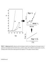
FIGURE 1.8

Frequency scans.

Frequency scans are one of the less often used methods in DMA. Frequency responses depend
on molecular structure and can be used to probe the molecular weight and distribution of the material. Properties such as relative

tack (stickiness) and peel (resistance to removal) responses can also be studied.
©2002 CRC Press LLC


©1999 CRC Press LLC

material as a function of temperature, we can also use DMA to quickly look at the
effect of shear rate or frequency on viscosity. For example, a polymer melt can be
scanned in a DMA for the effect of frequency on viscosity in less than 2 hours over
a range of 0.01 Hz to 200 Hz. A capillary rheometer study for similar rates would
take days. For a hot melt adhesive, we may need to see the low frequency modulus
(for stickiness or tack) as well as the high frequency response (for peel resistance).

23

We need to keep the material fluid enough to fill the pores of the substrate without
the elasticity getting so low the material pulls out of the pores too easily. By scanning
across a range of frequencies (Figure 1.8), we can collect information about the
elasticity and flow of the adhesive as

E

¢

and

h

* at the temperature of interest.
The frequency behavior of materials can also give information on molecular

structure. The crossover point between either

E

¢

and

h

* or between

E

¢

and

E

≤

can
be related to the molecular weight

24

and the molecular weight distribution

25

by the
Doi–Edwards theory. As a qualitative assessment of two or more samples, this
crossover point allows a fast comparison of samples that may be difficult or impos-
sible to dissolve in common solvents. In addition, the frequency scan at low fre-
quency will level off to the zero-shear plateau (Figure 1.9). In this region, changes
in frequency do not result in a change in viscosity because the rate of deformation
is too low for the chains to respond. A similar effect, the infinite shear plateau, is
found at very high frequencies. The zero-shear plateau viscosity can be directly
related to molecular weight, above a critical molecular weight by
(1.1)
where

k

is a material specific constant. This method has been found to be as accurate
as gel permeation chromatography (GPC) over a very wide range of molecular
weights for the polyolefins.

27

Frequency data are often manipulated in various ways to extend the range of
the analysis by exploiting the Boltzmann superposition principle.

28

Master curves
from superpositioning strain, frequency, time, degree of cure, humidity, etc., allow
one to estimate behavior outside the range of the instrument or of the experimenter’s
patience.

29

Like all accelerated aging and predictive techniques, one needs to remem-
ber that this is a bit like forecasting the weather, and care is required.

17

1.4 CREEP–RECOVERY TESTING

Finally, most DMAs on the market also allow creep–recovery testing. Creep is one
of the most fundamental tests of material behavior and is directly applicable to a
product performance.
30
We discuss this in Chapter 3 as part of the review of basic
principles, as it is the basic way to study polymer relaxation. Creep–recovery testing
is also a very powerful analytical tool. These experiments allow you to examine a
material’s response to constant load and its behavior on removal of that load. For
example, how a cushion on a chair responds to the body weight of the occupant,
how long it takes to recover, and how many times it can be sat on before it becomes
permanently compressed can all be studied by creep–recovery testing. The creep
h=
()
kM
34,

©1999 CRC Press LLC
quantifying the data can be used, as shown in Figure 1.10,
33
and will be discussed

in Chapter 3. Comparing materials after multiple cycles can be used to magnify the
differences between materials as well as predict long-term performance (Figure
1.11). Repeated cycles of creep–recovery show how the product will wear in the
real world, and the changes over even three cycles can be dramatic. Other materials,
such as a human hair coated with commercial hair spray, may require testing for
over a hundred cycles. Temperature programs can be applied to make the test more
closely match what the material is actually exposed to in end use. This can also be
done to accelerate aging in creep studies by using oxidative or reductive gases, UV
exposure, or solvent leaching.
34
1.5 ODDS AND ENDS
Any of these tests mentioned above can be done in controlled-environment con-
ditions to match the operating environment of the samples. Examples include
hydrogels tested in saline,
35
fibers in solutions,
36
and collagen in water.
37
UV light
can be used to cure samples
38
to mimic processing or operating conditions. A
specialized example of environmental testing is shown in Figure 1.12, where the
position control feature of a DMA is exploited to perform a specialized stress
relaxation experiment called constant gauge length (CGL) testing. The response
of the fibers is greatly affected by the solution it is tested in. Similar tests in both
dynamic and static modes are used in the medical, automotive, and cosmetic
industries. The adaptability of the DMA to match real-world conditions is yet
another advantage of the technique. The DMA’s ability to give insight into the

molecular structure and to predict in-service performance makes it a necessary
part of the modern thermal laboratory.
FIGURE 1.10 Creep–recovery testing. Creep–recovery experiments allow the determina-
tion of properties at equilibrium like modulus, E
e
, and viscosity, h
e
. These values allow the
prediction of material behavior under conditions that mimic real life applications.

2

©1999 CRC Press LLC

Basic Rheological
Concepts Stress, Strain,
and Flow

The term rheology seems to generate a slight sense of terror in the average worker
in materials. Rheology is defined as the study of the deformation and flow of
materials. The term was coined by Bingham to describe the work being done in
modeling how materials behave under heat and force. Bingham felt that chemists
would be frightened away by the term “continuum mechanics,” which was the name
of the branch of physics concerned with these properties.

1

This renaming was one
of science’s less successful marketing ploys, as most chemists think rheology is
something only done by engineers with degrees in non-Newtonian fluid mechanics,

and mostly likely in dark rooms.
More seriously, rheology does have an undeserved reputation of requiring a large
degree of mathematical sophistication. Parts of it do require a familiarity with
mathematics. However, many of the principles and techniques are understandable
to anyone who survived physical chemistry. Enough understanding of its principles
to use a DMA and successfully interpret the results doesn’t require even that much.
For those who find they would like to see more of the field, Chris Mascosko of
University of Minnesota has published the text of his short course,

2

and this is a
very readable introduction. We are now going to take a nonmathematical look at the
basic principles of rheology so we have a common terminology to discuss DMA.
This discussion is an elaboration of a lecture given by the author at University of
Houston called “Rheology for the Mathematically Insecure.”

2.1 FORCE, STRESS, AND DEFORMATION

If you apply a force to a sample, you get a deformation of the sample. The force,
however, is an inexact way of measuring the cause of the distortion. Now we know
the force exerted by a probe equals the mass of the probe (

m

) times its acceleration
(

a

). This is given as
(2.1)
However, force doesn’t give the true picture, or rather it gives an incomplete picture.
For example, which would you rather catch? A 25-lb medicine ball or a hardball
with 250 ft-lb of force? The above equation tells the force exerted by a 25-lb medicine
ball moving at 10 ft/s is equal to the force exerted by a hardball (0.25 lb) at 1000
Fma=*

©1999 CRC Press LLC

ft/s! We expect that the impact from the hardball is going to do more damage. This
damage is called a deformation.
So what we really need to include is a measure of the area of impact for the
example above. The product of a force (

F

) across an area (

A

) is a stress,



s

. The
stress is normally given in either pounds per square inch (psi) or pascals and can
be calculated for the physical under study. If we assume the medicine ball has an

area of impact equivalent to a 1-ft diameter, while the superball’s is 1 in., we can
calculate the stress by
(2.2)
Figure 2.1 gives a visual interpretation of the results. Despite the forces being
equal at 250 ft-lb, the stress seen by the sample varies from 250 psi to 2000 psi. If
we program a test in forces and our samples are not exactly the same size, the results
will differ because the stresses are different. This occurs even in the linear viscoelas-
tic region,

3

though in the nonlinear region the effects are magnified. While stress
gives a more realistic view of the material environment, in real life most people
choose to operate their instruments in forces. This allows you to track your instru-
ments limits more easily than having to remember the maximum stress in each
geometry would. However, it is important to realize that stress is what is affecting
the material, not force.
The applied stress causes a deformation of the material, and this deformation is
called a strain,



g

. A mnemonic for the difference is to remember that if your boss
is under a lot of stress, his personality changes are a strain. Strain is calculated as
(2.3)
where Y is the original sample dimension and

D

Y is the change in that dimension
under stress. This is often multiplied by 100 and expressed as percent of strain.
Applying a stress to a sample and recording the resultant strain is a commonly used
technique. Going back to the balls above, the different stresses can cause very
different strains in the material, be it a sheet of plastic or your catching hand. Figure
2.2 shows how some strains are calculated.

2.2 APPLYING THE STRESS

How the stress is applied can also affect the deformation of the material. Without
considering yet how changes in the material’s molecular structure or processing
enter the picture, we can see different behavior depending how a static stress

4

is
applied and what mode of deformation is used. Figure 2.3 summarizes the main
ways of applying a static stress. If we consider the basic stress–strain experiment
from materials testing, we increase the applied stress over time at a constant stress
rate ( ).

5

As shown in Figure 2.3a, we can track the change in strain as a function
of stress. This is done at constant temperature and generates the stress–strain curve.
Classically, this experiment was done by a strain-controlled instrument, where one

s=FA/
g=DYY

˙
s

©1999 CRC Press LLC

be looked at as brackets on the region of DMA testing. In traditional stress–strain
curves, we are concerned mainly with the elastic response of a material. This
behavior can be described as what one sees when you stress a piece of tempered
steel to an small degree of strain. The model we use to describe this behavior is the
spring, and Hooke’s Law relates the stress to the strain of a spring by a constant,

k.

This is graphically shown in Figure 2.6.
Hooke’s law states that the deformation or strain of a spring is linearly related
to the force or stress applied by a constant specific to the spring. Mathematically,
this becomes
(2.4)
where

k

is the spring constant. As the spring constant increases, the material becomes
stiffer and the slope of the stress–strain curve increases. As the initial slope is also
Young’s modulus, the modulus would also increase. Modulus, then, is a measure of
a material’s stiffness and is defined as the ratio of stress to strain. For an extension
system, we can then write the modulus,

E,

as
(2.5)
If the test is done in shear, the modulus denoted by

G

and in bulk as

B.

If we
then know the Poisson’s ratio,

n

, which is a measure of how the material volume
changes with deformation when pulled in extension, we can also convert one mod-
ulus into another (assuming the material is isotropic) by
(2.6)

FIGURE 2.5

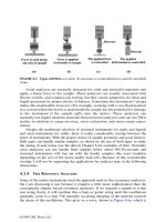
Modes of deformation.

Geometric arrangements or methods of applying stress
are shown. All of bottom fixtures are stationary. Bulk is 3-D compression, where sides are
restrained from moving.
sg=*k
Edd=se
EG B=-=-21 312() ( )nn

©1999 CRC Press LLC

or weak or strong. These combinations are shown in Figure 2.9. Interestingly, as the
testing temperature is increased, a polymer’s response moves through some or all
of these curves (Figure 2.10a). This change in response with temperature leads to
the need to map modulus as a function of temperature (Figure 2.10b) and represents
another advantage of DMA over isothermal stress–strain curves. Before we discuss
that, we need to explain the curvature seen in what Hooke’s law says should be a
straight line.

2.4 LIQUID-LIKE FLOW OR THE VISCOUS LIMIT

To explain the curvature in the stress–strain curves of polymers, we need to look at
the other end of the material behavior continuum. The other limiting extreme is
liquid-like flow, which is also called the Newtonian model. We will diverge a bit
here, to talk about the behavior of materials as they flow under applied force and
temperature.

10

We will begin to discuss the effect of the rate of strain on a material.
Newton defined the relationship by using the dashpot as a model. An example of a
dashpot would be a car’s shock absorber or a French press coffee pot. These have
a plunger header that is pierced with small holes through which the fluid is forced.
Figure 2.11 shows the response of the dashpot model. Note that as the stress is
applied, the material responds by slowly flowing through the holes. As the rate of
the shear is increased, the rate of flow of the material also increases. For a Newtonian
fluid, the stress–strain rate curve is a straight line, which can be described by the
following equation:

(2.8)

FIGURE 2.7 Stress–strain curves by geometry.

The stress–strain curves vary depending
on the geometry used for the test. Stress-strain curves for (a) tensile and (b) compressive are
shown.
shgh
g
== ∂
∂
˙
t

©1999 CRC Press LLC

observed in suspensions and slurries. Let’s just consider a polymer melt, as shown
in Figure 2.13, under a shearing force. Initially, a plateau region is seen at very low
shear rates or frequency. This region is also called the zero-shear plateau. As the
frequency (rate of shear) increases, the material becomes nonlinear and flows more.
This continues until the frequency reaches a region where increases in shear rate no
longer cause increased flow. This “infinite shear plateau” occurs at very high fre-
quencies.
Like with solids, the behavior you see is dependent on how you strain the
material. In shear and compression, we see a thinning or reduction in viscosity
(Figure 2.14). If the melt is tested in extension, a thickening or increase in the
viscosity of the polymer is observed. These trends are also seen in solid polymers.
Both a polymer melt and a polymeric solid under frequency scans show a low-
frequency Newtonian region before the shear thinning region. When polymers are
tested by varying the shear rate, we run into four problems that have been the drivers

for much of the research in rheology and complicate the life of polymer chemists.
These four problems are defined by C. Macosko

11

as (1) shear thinning of
polymers, (2) normal forces under shear, (3) time dependence of materials, and (4)
extensional thickening of melts. The first two can be solved by considering Hooke’s
Law and Newton’s Law in their three-dimensional forms.

12

Time dependence can
be addressed by linear viscoelastic theory. Extensional thickening is more difficult,
and the reader is referred to one of several references on rheology

13

if more infor-
mation is required.

2.5 ANOTHER LOOK AT THE STRESS–STRAIN CURVES

Before our discussion of flow, we were looking at a stress–strain curve. The curves
of real polymeric materials are not perfectly linear, and a rate dependence is seen.

FIGURE 2.12

Non-Newtonian behavior in solutions.

The major departures from Newto-
nian behavior are shown in the figure.