Dynamic Mechanical Analysis part 6 pdf
Bạn đang xem bản rút gọn của tài liệu. Xem và tải ngay bản đầy đủ của tài liệu tại đây (146.32 KB, 11 trang )
©1999 CRC Press LLC
Finally, one needs to check both the temperature accuracy and the furnace
control. I do this in one run by programming a cycle with 2-minute isothermal holds
at 100°C and 200°C and a 10°C per minute ramp between the holds. A sample of
indium is loaded under the probe and the analyzer stabilized at 95°C. After the run
is complete, one can check both temperature performance (Figure 4.16c) and tem-
perature accuracy (Figure 4.16d).
NOTES
1. This explanation was developed in terms of stress control and tensile stress, instead
of the shear strain and strain control normally used. For more detailed development,
see one of the following: L. Sperling, Introduction to Physical Polymer Science, 2nd
ed., Wiley, New York, 1996. L. Nielsen et al., Mechanical Properties of Polymers
and Composites, Marcel-Dekker, New York, 1996. J. Ferry, Viscoelastic Properties
of Polymers, Wiley, New York, 1980. The nice thing is the software does all this today
and you just need to understand how it works so you realize exactly what you are
doing.
2. J. Ferry, Viscoelastic Properties of Polymers, Wiley, New York, 1980, Ch. 5–7.
3a. R. Armstrong, B. Bird, and O. Hassager, Dynamics of Polymer Fluids, vol. 1, Fluid
Mechanics, 2nd ed., Wiley, New York, 1987, pp.151–153.
3b. D. Holland, J. Rheology, 38(6), p. 1941, 1994.
4. J. Gillham in Developments in Polymer Characterizations, vol. 3, J. Dworkins, Ed.,
Applied Science Publisher, Princeton, 1982, pp. 159–227. J. Gillham and J. Enns,
TRIP, 2(12), 406, 1994.
5. U. Zolzer and H-F. Eicke, Rheologia Acta, 32, 104, 1993.
6. N. McCrum et al., Anelastic and Dielectric Properties of Polymeric Solids, Dover,
New York, 1992, pp.192–200.
7. W. Young, Roark’s Formulas for Stress and Strain, McGraw-Hill, New York, 1989.
8. P. Zoller and Y. Fakhreddine, Thermochim. Acta, 238, 397, 1994. P. Zoller and D.
Walsh, Standard Pressure-Volume-Temperature Data for Polymers, Technomic Pub-
lishing, Lancaster, PA 1995.
9. See for example the instrument manuals written by Rheometric Sciences of Piscat-
away, NJ, where inertia affects are discussed at length.
10. C. Macosko, Rheology, VCH Publishers, New York, 1994, Ch. 5.
5
©1999 CRC Press LLC
Time–Temperature Scans:
Transitions in Polymers
One of most common uses of the DMA for users from a thermal analysis background
is the measurement of the various transitions in a polymer. A lot of users exploit
the greater sensitivity of the DMA to measure
T
g
’s undetectable by the differential
scanning calorimeter (DSC) or the differential thermal analyzer (DTA). For more
sophisticated users, DMA temperature scanning techniques let you investigate the
relaxation processes of a polymer. In this chapter, we will look at how time and
temperature can be used to study the properties of polymers. We will address curing
studies separately in Chapter 6.
5.1 TIME AND TEMPERATURE SCANNING IN THE DMA
If we start with a polymer at very low temperature and oscillate it at a set frequency
while increasing the temperature, we are performing a temperature scan (Figure
5.1a). This is what most thermal analysts think of as a DMA run. Similarly, we
could also hold the material at a set temperature and see how its properties change
over time (Figure 5.1b).
Experimentally we need to be concerned with the temperature accuracy and the
thermal control of the system, as shown in Figure 5.2. This is one of the most
commonly overlooked areas experimentally, as poor temperature control is often
accepted to maintain large sample size. A large sample means that there will be a
temperature difference across the specimen, which can result in anomalies such as
dual glass transitions in a homopolymer.
1
In his Polymer Fluids Short Course,
2
Bird
describes experiments where measuring the temperature at various points in a large
parallel plate experiment shows a 15
∞ C difference from the plate edge to the center.
Large samples require very slow heating rates and hide local differences. This is
especially true in post-cure studies. A smaller sample permits a smaller furnace,
which is inherently more controllable. Also, smaller sample size allows the section-
ing of specimens to see how properties vary across a specimen.
It is often very difficult to examine one specimen across the whole range of
interest with only one experiment or one geometry. Materials are very stiff and brittle
at low temperatures and soft near the melt, so very different conditions and fixtures
may be required. Some analyzers use sophisticated control loops
3
to address this
problem, but often it is best handled doing multiple runs.
5.2 TRANSITIONS IN POLYMERS: OVERVIEW
The thermal transitions in polymers can be described in terms of either free volume
changes
4
or relaxation times.
5
While the latter tends to be preferred by engineers and
©1999 CRC Press LLC
rheologists in contrast to chemist and polymer physicists who lean toward the former,
both descriptions are equivalent. Changes in free volume,
v
f
, can be monitored as a
volumetric change in the polymer; by the absorption or release of heat associated with
that change; the loss of stiffness; increased flow; or by a change in relaxation time.
The free volume of a polymer,
v
f
, is known to be related to viscoelasticity,
6
aging,
7
penetration by solvents,
8
and impact properties.
9
Defined as the space a molecule has
for internal movement, it is schematically shown in Figure 5.3a. A simple approach
to looking at free volume is the crankshaft mechanism,
10
where the molecule is
(a) Free Volume
(b) Crankshaft Model
FIGURE 5.3
Free volume,
v
f
, in polymers: (a) the relationship of free volume to transitions,
and (b) a schematic example of free volume and the crankshaft model. Below the
T
g
in (a)
various paths with different free volumes exist depending on heat history and processing of
the polymer, where the path with the least free volume is the most relaxed. The crankshaft
model (b) shows the various motions of a polymer chain. Unless enough free volume exists,
the motions cannot occur.
©1999 CRC Press LLC
imagined as a series of jointed segments. From this model, we can simply describe
the various transitions seen in a polymer. Other models exist that allow for more
precision in describing behavior; the best seems to be the Doi–Edwards model.
11
Aklonis and Knight
12
give a good summary of the available models, as does Rohn.
13
The crankshaft model treats the molecule as a collection of mobile segments
that have some degree of free movement. This is a very simplistic approach, yet
very useful for explaining behavior. As the free volume of the chain segment
increases, its ability to move in various directions also increases (Figure 5.3b). This
increased mobility in either side chains or small groups of adjacent backbone atoms
results in a greater compliance (lower modulus) of the molecule. These movements
have been studied, and Heijboer classified
b
and
g
transitions by their type of
motions.
14
The specific temperature and frequency of this softening help drive the
end use of the material.
As we move from very low temperature, where the molecule is tightly com-
pressed, we pass first through the solid state transitions. This process is shown in
Figures 5.4 (6). As the material warms and expands, the free volume increases so
that localized bond movements (bending and stretching) and side chain movements
can occur. This is the gamma transition,
T
g
, which may also involve associations
with water.
15
As the temperature and the free volume continue to increase, the whole
side chains and localized groups of four to eight backbone atoms begin to have
enough space to move and the material starts to develop some toughness.
16
This
transition, called the beta transition
T
b
, is not as clearly defined as we are describing
here (Figures 5.4 (5)). Often it is the
T
g
of a secondary component in a blend or of
a specific block in a block copolymer. However, a correlation with toughness is seen
empirically.
17
As heating continues, we reach the
T
g
or glass transition, where the chains in
the amorphous regions begin to coordinate large-scale motions (Figure 5.4 (4)). One
classical description of this region is that the amorphous regions have begun to melt.
Since the
T
g
only occurs in amorphous material, in a 100% crystalline material we
would see not a
T
g
. Continued heating bring us to the
T
a
* and
T
ll
(Figure 5.4 (3)).
The former occurs in crystalline or semicrystalline polymer and is a slippage of the
crystallites past each other. The latter is a movement of coordinated segments in the
amorphous phase that relates to reduced viscosity. These two transitions are not
accepted by everyone, and their existence is still a matter of some disagreement.
Finally, we reach the melt (Figure 5.4 (2)) where large-scale chain slippage occurs
and the material flows. This is the melting temperature,
T
m
. For a cured thermoset,
nothing happens after the
T
g
until the sample begins to burn and degrade because
the cross-links prevent the chains from slipping past each other.
This quick overview gives us an idea of how an idealized polymer responds. Now
let us go over these transitions in more detail with some examples of their applications.
The best general collection of this information is still McCrum’s 1967 text.
10
5.3 SUB-
T
g
TRANSITIONS
The area of sub-
T
g
or higher-order transitions has been heavily studied,
18
as these
transitions have been associated with mechanical properties. These transitions can
©1999 CRC Press LLC
sometimes be seen by DSC and TMA, but they are normally too weak or too
broad for determination by these methods. DMA, Dielectric Analysis (DEA), and
similar techniques are usually required.
19
Some authors have also called these
types of transitions second-order transitions to differentiate them from the primary
transitions of
T
m
and
T
g
, which involve large sections of the main chains.
20
Boyer
reviewed the
T
b
in 1968,
21
and pointed out that while a correlation often exists,
the
T
b
is not always an indicator of toughness. Bershtein has reported that this
transition can be considered the “activation barrier” for solid-phase reactions,
deformation, flow or creep, acoustic damping, physical aging changes, and gas
diffusion into polymers, as the activation energies for the transition and these
processes are usually similar.
22
The strength of these transitions is related to how
strongly a polymer responsed to those processes. These sub-
T
g
transitions are
associated with the materials properties in the glassy state. In paints, for example,
peel strength (adhesion) can be estimated from the strength and frequency depen-
dence of the sub-ambient beta transition.
23
Nylon 6,6 shows a decreasing tough-
ness, measured as impact resistance, with declining area under the
T
b
peak in the
tan
d
curve. Figure 5.5 shows the relative differences in the
T
b
compared to the
T
g
for a high-impact and low-impact nylon. It has been shown, particularly in
cured thermosets, that increased freedom of movement in side chains increases
the strength of the transition. Cheng and colleagues report in rigid rod polyimides
that the beta transition is caused by the noncoordinated movement of the diamine
groups, although the link to physical properties was not investigated.
24
Johari and
colleagues have reported in both mechanical
25
and dielectric studies
26
that both
the
b
and
g
transitions in bisphenol-A-based thermosets depend on the side chains
and unreacted ends, and that both are affected by physical aging and postcure.
Nelson has reported that these transitions can be related to vibration damping.
27
This is also true for acoustical damping.
28
In both of these cases, the strength of
the beta transition is taken as a measurement of how effectively a polymer will
absorb vibrations. There is some frequency dependence involved in this, which
will be discussed later in Section 5.7.
Boyer
29
and Heijboer
14
showed that this information needs to be considered with
care, as not all beta transitions correlate with toughness or other properties (Figure
5.6). This can be due to misidentification of the transition or to the fact that the
transition does not sufficiently disperse energy. A working rule of thumb
30
is that
the beta transition must be related to either localized movement in the main chain
or very large side chain movement to sufficiently absorb enough energy. The rela-
tionship of large side chain movement and toughness has been extensively studied
in polycarbonate by Yee,
31
as well as in many other tough glassy polymers.
32
Less use is made of the
T
g
transitions, and they are mainly studied to understand
the movements occurring in polymers. Wendorff reports that this transition in poly-
arylates is limited to inter- and intramolecular motions within the scale of a single
repeat unit.
33
Both McCrum et al.
10
and Boyd
34
similarly limited the
T
g
and
T
d
to
very small motions either within the molecule or with bound water. The use of what
is called 2D-IR, which couples an Fourier Transform Infrared Spectrometer (FTIR)
and a DMA to study these motions, is a topic of current interest.
35
©1999 CRC Press LLC
5.4 THE GLASS TRANSITION (
T
g
OR
T
aa
aa
)
As the free volume continues to increase with increasing temperature, we reach the
glass transition,
T
g
, where large segments of the chain start moving. This transition
is also called the alpha transition,
T
a
. The
T
g
is very dependent on the degree of
polymerization up to a value known as the critical
T
g
or the critical molecular
weight.
36
Above this value, the
T
g
typically becomes less dependent on molecular
weight. The
T
g
represents a major transition for many polymers, as physical prop-
erties changes drastically as the material goes from a hard glassy to a rubbery state.
It defines one end of the temperature range over which the polymer can be used,
often called the operating range of the polymer, and examples of this range are
shown in Figure 5.7. For where strength and stiffness are needed, it is normally the
upper limit for use. In rubbers and some semicrystalline materials such as polyeth-
ylene and polypropylene, it is the lower operating temperature. Changes in the
temperature of the
T
g
are commonly used to monitor changes in the polymer such
as plasticizing by environmental solvents and increased cross-linking from thermal
or UV aging (Figure 5.8).
The
T
g
of cured materials or thin coatings is often difficult to measure by other
methods, and more often than not the initial cost justification for a DMA is in
measuring a hard-to-find
T
g
. While estimates of the relative sensitivity of DMA to
DSC or DTA vary, it appears that DMA is 10 to 100 times more sensitive to the
changes occurring at the
T
g
. The
T
g
in highly cross-linked materials can easily be
seen long after the
T
g
has become too flat and diffuse to be seen in the DSC (Figure
5.9a). A highly cross-linked molding resin used for chip encapsulation was run by
(a)
FIGURE 5.7
Operating range by DMA.
Definition of operating range based on position
of
T
g
in (a) polycarbonate, (b) epoxy, and (c) polypropylene.
©1999 CRC Press LLC
both methods, and the DMA is able to detect the transition after it is undetectable
in the DSC. This is also a known problem with certain materials such as medical-
grade urethanes and very highly crystalline polyethylenes.
The method of determining the
T
g
in the DMA can be a manner for disagreement,
as at least five ways are in current use (Figure 5.9b). This is not unusual, as DSC
has multiple methods too (Figure 5.9c). Depending on the industry standards or
(b)
(c)
FIGURE 5.7
(
Continued
).
©1999 CRC Press LLC
entanglements (M
e
)
37
or cross-links. The molecular weight between entanglements
is normally calculated during a stress–relaxation experiment, but similar behavior
is observed in the DMA (Figure 5.11). The modulus in the plateau region is pro-
portional to either the number of cross-links or the chain length between entangle-
ments. This is often expressed in shear as
(5.1)
where G¢ is the modulus of the plateau region at a specific temperature, r is the
polymer density, and M
e
is the molecular weight between entanglements. In practice,
(b)
FIGURE 5.8 (Continued
).
GRTM¢@(r )
e
©1999 CRC Press LLC
the relative modulus of the plateau region tells us about the relative changes in M
e
or the number of cross-links compared to a standard material.
The rubbery plateau is also related to the degree of crystallinity in a material,
although DSC is a better method for characterizing crystallinity than DMA.
38
This
is shown in Figure 5.12. Also as in the DSC, we can see evidence of cold crystal-
lization in the temperature range above the T
g
(Figure 5.13). That is one of several
(b)
(c)
FIGURE 5.9 (Continued). (b) Multiple methods of determining the T
g
are shown for the
DMA. The temperature of the T
g
varies up 10°C in this example, depending on the value
chosen. Differences as great as 25°C have been reported. (c) Four of the methods used to
determine the T
g
in DSC are shown. The half-height and half-width methods are not included.
©1999 CRC Press LLC
FIGURE 5.10 Stress relief at the T
g
in the DMA. The overshoot is similar to that seen in the DSC and is caused by molecular rearrangements
that occur due to the increased free volume at the transition.
©1999 CRC Press LLC
transitions that can be seen in the rubbery plateau region. This crystallization occurs
when the polymer chains have been quenched (quickly cooled) into a highly disor-
dered state. On heating above the T
g
, these chains gain enough mobility to rearrange
into crystallites, which causes a sometimes-dramatic increase in modulus (Figure
5.13). DSC or its temperature-modulated variant, dynamic differential scanning
calorimetry (DDSC), can be used to confirm this.
39
The alpha star transition, T
a
*, the liquid–liquid transition, T
ll
, the heat-set tem-
perature, and the cold crystallization peak are all transitions that can appear on the
rubbery plateau. In some crystalline and semicrystalline polymers, a transition is
seen here called the T
a
*.
40
Figure 5.14 shows this in a sample of polypropylene. The
alpha star transition is associated with the slippage between crystallites and helps
extend the operating range of a material above the T
g
. This transition is very sus-
ceptible to processing-induced changes and can be enlarged or decreased by the
applied heat history, processing conditions, and physical aging.
41
The T
a
* has been
used by fiber manufacturers to optimize properties in their materials.
In amorphous polymers, we instead see the T
ll
, a liquid–liquid transition asso-
ciated with increased chain mobility and segment–segment associations.
42
This order
is lost when the T
ll
is exceeded and regained on cooling from the melt
.
Boyer reports
that, like the T
g
, the appearance of the T
ll
is affected by the heat history.
43
The T
ll
is
also dependent on the number-average molecular weight, M
n
, but not on the weight-
average molecular weight, M
w
. Bershtein suggests that this may be considered as
quasi-melting on heating or the formation of stable associates of segments on
cooling.
44
While this transition is reversible, it is not always easy to see, and Boyer
spent many years trying to prove it was real.
45
Not everyone accepts the existence
of this transition. This transition may be similar to some of the data from temperature-
modulated DSC experiments showing a recrystallization at the start of the melt.
46
In both cases, some subtle changes in structure are sometimes detected at the start
of melting. Following this transition, a material enters the terminal or melting region.
Depending on its strength, the heat-set temperature can also seen in the DMA.
While it is normally seen in either a TMA or a CGL experiment (Figure 5.15), it
will sometimes appear as either a sharp drop in modulus (E¢) or an abrupt change
in probe position. Heat set is the temperature at which some strain or distortion is
induced into polymeric fibers to change their properties, such as to prevent a nylon
rug from feeling like fishing line. Since heating above this temperature will erase
the texture, and you must heat polyesters above the T
g
to dye them, it is of critical
importance to the fabric industry. Many final properties of polymeric products
depend on changes induced in processing.
47
5.6 THE TERMINAL REGION
On continued heating, the melting point, T
m
, is reached. The melting point is chains
where the fee volume has increased so that the slide can past each other and the
material flows. This is also called the terminal region. In the molten state, this ability
to flow is dependent on the molecular weight of the polymer (Figure 5.16). The melt
of a polymer material will often show changes in temperature of melting, width of