Dynamic Mechanical Analysis part 8 potx
Bạn đang xem bản rút gọn của tài liệu. Xem và tải ngay bản đầy đủ của tài liệu tại đây (157.77 KB, 11 trang )
©1999 CRC Press LLC
FIGURE 6.3
Effects of staging on the curing of resins.
Staging is done to improve handling properties during lay-up but also changes the cure profile.
©1999 CRC Press LLC
Another special area of concern is paints and coatings,
9
where the material is
used in a thin layer. This can be addressed experimentally by either employing a
braid as above or coating the material on a thin sheet of metal. The metal is often
run first and its scan subtracted from the coated sheet’s scan to leave only the scan
of the coating. This is also done with thin films and adhesive coatings.
A sample cure profile for a commercial two-part epoxy resin is shown in Figure
6.6. From this scan, we can determine the minimum viscosity (
h
*
min
), the time to
h
*
min
and the length of time it stays there, the onset of cure, the point of gelation
where the material changes from a viscous liquid to a viscoelastic solid, and the
beginning of vitrification. The minimum viscosity is seen in the complex viscosity
curve and is where the resin viscosity is the lowest. A given resin’s minimum
viscosity is determined by the resin’s chemistry, the previous heat history of the
resin, the rate at which the temperature is increased, and the amount of stress or
stain applied. Increasing the rate of the temperature ramp is known to decrease the
h
*
min
, the time to
h
*
min
, and the gel time. The resin gets softer faster, but also cures
faster. The degree of flow limits the type of mold design and when as well as how
much pressure can be applied to the sample. The time spent at the minimum viscosity
plateau is the result of a competitive relationship between the material’s softening
or melting as it heats and its rate of curing. At some point, the material begins curing
faster than it softens, and that is where we see the viscosity start to increase.
As the viscosity begins to climb, we see an inversion of the
E
≤
and
E
¢
values
as the material becomes more solid-like. This crossover point also corresponds to
where the tan
d
equals 1 (since
E
¢
=
E
≤
at the crossover). This is taken to be the gel
point,
10
where the cross-links have progressed to forming an “infinitely” long net-
FIGURE 6.4
Relationship of
T
g
to cure time
and the stages of a cure. Note that for
thermosets, it is often difficult to impossible to see the
T
g
by DSC in the latter half of region 3.
©1999 CRC Press LLC
(a)
(b)
FIGURE 6.5
T
g
and
E¢¢
¢¢
for post-cure times.
(a) Data collected by DMA on chip encapsu-
lation material plotted as time of post cure vs. measured values listed in the table.
T
g
was
measured as the peak of the tan
d
, the onset of tan
d
, and the onset of the drop in
E
¢
. Storage
modulus was measured at 50
∞
C and is reported as
e
9
Pa. (b) The measurement of
T
g
by tan
d
peak values for the data in (a) is shown. All the
T
g
’s except the 0 hour of post-cure
T
g
were
undetectable by DSC.
©1999 CRC Press LLC
this again in Chapter 7.) At the gel point, the frequency dependence disappears
14
(see Figure 6.7). My own experience is that this value is only a few degrees different
from the one obtained in a normal scan and not worth the additional time. During
this rapid climb of viscosity in the cure, the slope for
h
* increase can be used to
calculate an estimated
E
act
(activation energy).
15
We will discuss this below, but the
fact that the slope of the curve here is a function of
E
act
is important. Above the gel
temperature, some workers estimate the molecular weight,
M
c
, between cross-links as
(6.1)
where
R
is the gas constant,
T
is the temperature in Kelvin, and
r
is the density. At
some point the curve begins to level off, and this is often taken as the vitrification
point,
T
vf
.
The vitrification point is where the cure rate slows because the material has
become so viscous that the bulk reaction has stopped. At this point, the rate of cure
slows significantly. The apparent
T
vf
, however, is not always real: any analyzer in
the world has an upper force limit. When that force limit is reached, the “topping
out” of the analyzer can pass as the
T
vf
.
Use of a combined technique such as
DMA–DEA
16
to see the higher viscosities, or removing a sample from parallel plate
and sectioning it into a flexure beam, is often necessary to see the true vitrification
point (Figure 6.8). A reaction can also completely cure without vitrifying and will
level off the same way. One should be aware that reaching vitrification or complete
cure too quickly could be as bad as too slowly. Often a overly aggressive cure cycle
will result in a weaker material, as it does not allow for as much network develop-
ment, but gives a series of hard (highly cross-linked) areas among softer (lightly
cross-linked) areas.
On the way to vitrification, I have marked a line at 10
6
Pa. s. This is the
viscosity of bitumen
17
and is often used as a rule of thumb for where a material
is stiff enough to support its own weight. This is a rather arbitrary point, but is
chosen to allow the removal of materials from a mold, and the cure is then
continued as a post-cure step. As an example, Table 6.1 gives the viscosities of
common materials. As we shall see below, the post-cure is often a vital part of
the curing process.
The cure profile is both a good predictor of performance as well as a sensitive
probe of processing conditions. We will discuss the former case under Section 6.4
below and the latter as part of Section 6.7. A final note on cure profiles is that a
volume change occurs during the cure.
18
This shrinkage of the resin is important
and can be studied by monitoring the probe position of some DMAs as well as by
TMA and dilatometry.
6.3 PHOTO-CURING
A photo-cure in the DMA is run by applying a UV light source to a sample that is
held at a specific temperature or subjected to a specific thermal cycle.
19
Photo-curing
is done for dental resin, contact adhesives, and contact lenses. UV exposure studies
are also run on cured and thermoplastic samples by the same techniques as photo-
GRTM¢= r
c
GRTM¢= r
c
©1999 CRC Press LLC
(a)
(b)
FIGURE 6.9
Photo-cure of a UV curing adhesive in the DMA.
Note the similarity to the
materials in Figure 6.1a and b.
©1999 CRC Press LLC
FIGURE 6.10
Multistep cure cycles:
A multiple step cure cycle with two ramps and two isothermal holds is used to model processing conditions.
Run on an RDA 2 by the author.
©1999 CRC Press LLC
collected. It is also how rubber samples are cross-linked, how initiated reactions are
run, and how bulk polymerizations are performed. Industrially, continuous processes,
as opposed to batch, require an isothermal approach. Figure 6.11 shows the isother-
mal cure of a rubber (a) and three isothermal polymerizations (b) that were used for
a kinetic study. UV light and other forms of nonthermal initiation also use isothermal
studies for examining the cure at a constant temperature.
6.6 KINETICS BY DMA
Several approaches have been developed to studying the chemorheology of thermo-
setting systems. MacKay and Halley (Table 6.2) recently reviewed chemorheology
and the more common kinetic models.
22
A fundamental method is the Williams–Lan-
del–Ferry (WLF) model,
23
which looks at the variation of
T
g
with degree of cure.
This has been used and modified extensively.
24
A common empirical model for
curing has been proposed by Roller.
25
This method will be discussed in depth, as
well as some of the variations on it.
Samples of the thermoset are run isothermally as described above, and the
viscosity versus time data are plotted as shown in Figure 6.11b. This is replotted in
Figure 6.12 as log
h
* vs. time in seconds, where a change in slope is apparent in
the curve. This break in the data indicates the sample is approaching the gel time.
From these curves, we can determine the initial viscosity,
h
o
and the apparent kinetic
factor,
k.
By plotting the log viscosity vs. time for each isothermal run, we get the
slope,
k,
and the viscosity at
t
= 0. The initial viscosity and
k
can be expressed as
(6.2)
(6.3)
Combining these allows us to set up the equation for viscosity under isothermal
conditions as
(6.4)
By replacing the last term with an expression that treats temperature as a function
of time, we can write
(6.5)
This equation can be used to describe viscosity–time profiles for any run where the
temperature can be expressed as a function of time. Returning to the data plotted in
Figure 6.12, we can determine the activation energies we need as follows. The plots
of the natural log of the initial viscosity (determined above) vs. 1/
T and the natural
hh
h
o
=
•
e
ERTD
hh
h
o
=
•
e
ERTD
kke
ERT
k
o
=
•
D
kke
ERT
k
o
=
•
D
ln ( ) lnhh
h
tERTtk e
ERT
k
=+ +
••
D
D
ln ( ) lnhh
h
tERTtk e
ERT
k
=+ +
••
D
D
ln ( , ) lnhh
h
Tt E RT ke dt
ERT
t
k
=+ +
••
Ú
D
D
0
ln ( , ) lnhh
h
Tt E RT ke dt
ERT
t
k
=+ +
••
Ú
D
D
0
©1999 CRC Press LLC
6.7 MAPPING THERMOSET BEHAVIOR: THE
GILLHAM–ENNS DIAGRAM
Another approach to attempt to fully understand the behavior of a thermoset was
developed by Gillham
30
and is analogous to the phase diagrams used by metallurgists.
The time-temperature–transition diagram (TTT) or the Gilham–Enns diagram (after
its creators) is used to track the effects of temperature and time on the physical state
of a thermosetting material. Figure 6.14 shows an example. These can be done by
running isothermal studies of a resin at various temperatures and recording the
changes as a function of time. One has to choose values for the various regions, and
Gillham has done an excellent job of detailing how one picks the T
g
, the glass, the
gel, the rubbery, and the charring regions.
31
These diagrams are also generated from
DSC data,
32
and several variants,
33
such as the continuous heating transformation
and conversion-temperature-property diagrams, have been reported. Surprisingly
easy to do, although a bit slow, they have not yet been accepted in industry despite
their obvious utility. A recent review
34
will hopefully increase the use of this
approach.
FIGURE 6.14 The Gillham–Enns or TTT diagram. (From J. K. Gillham and J. B. Enns,
Trends in Polymer Science, 2(12), 406–419, 1994. With permission from Elsevier Science.)
©1999 CRC Press LLC
6.8 QC APPROACHES TO THERMOSET
CHARACTERIZATION
Quality control (QC) is still one of the biggest applications of the DMA in industry.
For thermosets, this normally involves two approaches to examining incoming mate-
rials or checking product quality. First is the very simple approach of fingerprinting
a resin. Figure 6.15 shows this for two adhesives; a simple heating run under
standardized conditions allows one to compare the known good material with the
questionable material. This can be done as simply as described or by measuring
various quantities.
A second approach is to run the cure cycle that the material will be processed
under in production and check the key properties for acceptable values. Figure 6.16
shows three materials run under the same cycle. Note the differences in the minimum
viscosity, in the length and shape of the minimum viscosity plateau, the region of
increasing viscosity associated with curing, and both the time required to exceed
1 ¥ 10
6
Pa. s and to reach vitrification. These materials, sold for the same application,
would require very different cure cycles to process. If we estimate the activation
energy, E
act
, by taking the values of h* at various temperatures and plotting them
versus 1/T, we get very different numbers. (This is a fast way of estimating the E
act
,
where we will assume the viscosity obtained from the temperature ramp is close to
the initial viscosity of the Roller method. This is not a very accurate assumption,
but for materials cured under the same conditions, it works.) This indicates, as did
the shape of the cures, different times are required to complete the cures. The
differences in the minimum viscosity mean the material will have different flow
characteristics and, for the same pressure cycle, give different thicknesses. As dif-
ferent times are required to reach a viscosity equal to or exceeding 10
6
Pa. s, the
materials will need to be held for different times before they are solid enough to
FIGURE 6.15 QC comparisons. Fingerprinting of materials for QC is often done. Good
and bad hot melt adhesives were scanned using a constant heating rate cure profile.
©1999 CRC Press LLC
FIGURE 6.17 Results and analysis of a “gel” time test from a DMA run. Note the “gel time” here is really the time to vitrification, not gelation.
7
©1999 CRC Press LLC
Frequency Scans
Frequency scans are the most commonly used method to study melt behavior in the
DMA and, at the same time, the most neglected experiment for many users. DMA
users from a rheological or polymer engineering background depend on the DMA
to answer all sorts of questions about polymer melts. For many chemists and thermal
analysts using DMA, the frequency scan is an ill-defined technique associated with
a magical predictive method called time–temperature superposition. In this chapter,
we will attempt to clear away some of the confusion and explain why the frequency
dependence of a polymer is important.
7.1 METHODS OF PERFORMING A FREQUENCY SCAN
Frequency effects can be studied in various ways of changing the frequency: scanning
or sweeping across a frequency range, applying a selection of frequencies to a
sample, applying a complex wave form to the sample and solving its resultant strain
wave, or by free resonance techniques (see Figure 7.1). Special techniques are also
used to obtain collections of frequency data as a function of temperature for devel-
oping master curves and for studying the effect of frequency on temperature-driven
changes in the material.
To collect frequency data, the simplest and most common approach is to hold
the temperature constant and scan across the frequency range of interest. This may
be done at a series of isotherms to obtain a multiplex of curves. Alternatively, one
can sample a set collection of frequencies, like 1 Hz, 2.5 Hz, 5 Hz, and 10 Hz, that
give a good overview on a logarithmic graph. Sampling frequencies is often per-
formed with a simultaneous temperature scan to speed up data collection. However,
since two variables are changing at the same time, there are concerns that the data
are not accurate. At least two runs at different scan rates should be done so one can
factor out the effects of temperature from frequency. Ideally, frequency scans should
be done isothermally.
The application of a complex waveform allows very fast collection of data. By
combining a set of sine waves into one wave, data can be taken for multiple
frequencies in less than 30 seconds. Several approaches are used and have been
reviewed by Dealy and Nelson.
1
The user should be concerned that the test is
confined to the region where the Boltzmann superposition principle
2
holds for the
material. Free resonance techniques,
3
discussed in Chapter 4, can also be used.
To extend the range of frequency studies to very low or high frequencies outside
the instruments scanning range, data are often added from either creep or free
resonance experiments. Creep data provide results at very low rates of deformation,
while free resonance will provide results at the higher rates of deformation. The
latter can be obtained in a stress-controlled rheometer in a recovery experiment
4
or
from a specialized free resonance instrument.
3
The data from these experiments can
only be added if the material acts in these tests similarly to the way it acts in a