Engineering Tribology Episode 1 Part 3 pdf
Bạn đang xem bản rút gọn của tài liệu. Xem và tải ngay bản đầy đủ của tài liệu tại đây (694.17 KB, 25 trang )
PHYSICAL PROPERTIES OF LUBRICANTS 25
υ = πr
4
glt / 8LV = k(t
2
− t
1
) (2.15)
where:
υ is the kinematic viscosity [m
2
/s];
r is the capillary radius [m];
l is the mean hydrostatic head [m];
g is the earth acceleration [m/s
2
];
L is the capillary length [m];
V is the flow volume of the fluid [m
3
];
t is the flow time through the capillary, t = (t
2
− t
1
), [s];
k is the capillary constant which has to be determined experimentally by applying
a reference fluid with known viscosity, e.g. by applying freshly distilled water.
The capillary constant is usually given by the manufacturer of the viscometer.
Capillary
tube
Etched
rings
British Standard
U-tube viscometer
Capillary
tube
Capillary
tube
Etched
rings
Glass
strengthening
bridge
Kinematic viscometers
for transparent
fluids
for opaque
fluids
FIGURE 2.10 Typical capillary viscometers (adapted from [23]).
In order to measure the viscosity of the fluid by one of the viscometers shown in Figure 2.10,
the container is filled with oil between the etched lines. The measurement is then made by
timing the period required for the oil meniscus to flow from the first to the second timing
mark. This is measured with an accuracy to within 0.1 [s].
Kinematic viscosity can also be measured by so called ‘short tube’ viscometers. In the
literature they are also known as efflux viscometers. As in the previously described
viscometers, viscosity is determined by measuring the time necessary for a given volume of
fluid to discharge under gravity through a short tube orifice in the base of the instrument.
The most commonly used viscometers are Redwood, Saybolt and Engler. The operation
principle of these viscometers is the same, and they only differ by the orifice dimensions and
the volume of fluid discharged. Redwood viscometers are used in the United Kingdom,
Saybolt in Europe and Engler mainly in former Eastern Europe. The viscosities measured by
these viscometers are quoted in terms of the time necessary for the discharge of a certain
volume of fluid. Hence the viscosity is sometimes found as being quoted in Redwood and
TEAM LRN
26 ENGINEERING TRIBOLOGY
Saybolt seconds. The viscosity measured on Engler viscometers is quoted in Engler degrees,
which is the time for the fluid to discharge divided by the discharge time of the same volume
of water at the same temperature. Redwood and Saybolt seconds and Engler degrees can
easily be converted into centistokes as shown in Figure 2.11. These particular types of
viscometers, are gradually becoming obsolete, since they do not easily provide calculable
viscosity. A typical short tube viscometer is shown in Figure 2.12.
In order to extend the range of kinematic, Saybolt Universal, Redwood No. 1 and Engler
viscosity scales only (Figure 2.11), a simple operation is performed. The viscosities on these
scales which correspond to the viscosity between 100 and 1000 [cS] on the kinematic scale are
multiplied by a factor of 10 and this gives the required extension. For example:
4000
[cS] = 400 [cS] × 10 ≈ 1850 [SUS] × 10 = 18500 [SUS] ≈ 51 [Engler] × 10 = 510 [Engler]
2
2.5
3
3.5
4
4.5
5
6
7
8
9
10
15
20
25
30
35
40
45
50
60
70
80
90
100
150
200
250
300
350
400
450
500
600
700
800
900
1 000
2
2.5
3
3.5
4
4.5
5
6
7
8
9
10
15
20
25
30
35
40
45
50
60
70
80
90
100
150
200
250
300
350
400
450
500
600
700
800
900
1 000
Kinematic viscosity, cS
Saybolt universal seconds
Redwood Nº 1 seconds (standard)
Engler degrees
Saybolt furol seconds
Redwood Nº 2 seconds (admiralty)
Kinematic viscosity, cS
100
150
200
250
300
350
400
450
500
600
700
800
900
1 000
1 500
2 000
2 500
3 000
3 500
4 000
4 500
35
40
45
50
60
70
80
90
100
150
200
250
300
350
400
450
500
600
700
800
900
1 000
1 500
2 000
2 500
3 000
3 500
4 000
35
40
45
50
60
70
80
90
2
2.5
3
3.5
4
4.5
5
6
7
8
9
10
15
20
25
30
35
40
45
50
60
70
80
90
1.9
1.8
1.7
1.6
1.5
1.4
1.3
1.2
25
30
35
40
45
50
60
70
80
90
100
150
200
250
300
350
400
450
30
35
40
45
50
60
70
80
90
100
150
200
250
300
350
400
100
120
FIGURE 2.11 Viscosity conversion chart (compiled by Texaco Inc.).
Rotational Viscometers
Rotational viscometers are based on the principle that the fluid whose viscosity is being
measured is sheared between two surfaces (ASTM D2983). In these viscometers one of the
surfaces is stationary and the other is rotated by an external drive and the fluid fills the space
in between. The measurements are conducted by applying either a constant torque and
measuring the changes in the speed of rotation or applying a constant speed and measuring
TEAM LRN
PHYSICAL PROPERTIES OF LUBRICANTS 27
the changes in the torque. These viscometers give the ‘dynamic viscosity’. There are two
main types of these viscometers: rotating cylinder and cone-on-plate viscometers.
Stopper
Capillary
tube
Lubricant
sample
Water
bath
Overflow
rim
FIGURE 2.12 Schematic diagram of a short tube viscometer.
· Rotating Cylinder Viscometer
The rotating cylinder viscometer, also known as a ‘Couette viscometer’, consists of two
concentric cylinders with an annular clearance filled with fluid as shown in Figure 2.13. The
inside cylinder is stationary and the outside cylinder rotates at constant velocity. The force
necessary to shear the fluid between the cylinders is measured. The velocity of the cylinder
can be varied so that the changes in viscosity of the fluid with shear rate can be assessed. Care
needs to be taken with non-Newtonian fluids as these viscometers are calibrated for
Newtonian fluids. Different cylinders with a range of radial clearances are used for different
fluids. For Newtonian fluids the dynamic viscosity can be estimated from the formula:
η = M(1/r
b
2
− 1/r
c
2
) / 4πdω = kM / ω (2.16)
where:
η is the dynamic viscosity [Pas];
r
b
, r
c
are the radii of the inner and outer cylinders respectively [m];
M is the shear torque on the inner cylinder [Nm];
ω is the angular velocity [rad/s];
d is the immersion depth of the inner cylinder [m];
k is the viscometer constant, supplied usually by the manufacturer for each pair of
cylinders [m
-3
].
When motor oils are used in European and North American conditions, the oil viscosity
data at -18°C is required in order to assess the ease with which the engine starts. A specially
adapted rotating cylinder viscometer, known in the literature as the ‘Cold Cranking
Simulator’ (CCS), is used for this purpose (ASTM D2602). The schematic diagram of this
viscometer is shown in Figure 2.14.
TEAM LRN
28 ENGINEERING TRIBOLOGY
Driving motor
Pointer
Torsion
wire
Graduated
scale
Fluid
sample
ω
r
c
r
b
Inner cylinder
(stationary)
Outer cylinder
(rotating)
FIGURE 2.13 Schematic diagram of a rotating cylinder viscometer.
Overload clutch
Constant-power
motor drive
with tachometer
Coolant
(methanol)
in
Coolant
out
Nylon
block
Thermocouple
ω
Lubricant sample
Rotating
cylinder
Stationary
cylinder
FIGURE 2.14 Schematic diagram of a cold cranking simulator.
The inner cylinder is rotated at constant power in the cooled lubricant sample of volume
about 5 [ml]. The viscosity of the oil sample tested is assessed by comparing the rotational
speed of the test oil with the rotational speed of the reference oil under the same conditions.
The measurements provide an indication of the ease with which the engine will turn at low
temperatures and with limited available starting power. In the case of very viscous fluids,
two cylinder arrangements with a small clearance might be impractical because of the very
high viscous resistance; thus a single cylinder is rotated in a fluid and measurements are
calibrated against measurements obtained with reference fluids.
· Cone on Plate Viscometer
The cone on plate viscometer consists of a conical surface and a flat plate. Either of these
surfaces can be rotated. The clearance between the cone and the plate is filled with the fluid
TEAM LRN
PHYSICAL PROPERTIES OF LUBRICANTS 29
and the cone angle ensures a constant shear rate in the clearance space. The advantage of this
viscometer is that a very small sample volume of fluid is required for the test. In some of
these viscometers, the temperature of the fluid sample is controlled during tests. This is
achieved by circulating pre-heated or cooled external fluid through the plate of the
viscometer. These viscometers can be used with both Newtonian and non-Newtonian fluids
as the shear rate is approximately constant across the gap. The schematic diagram of this
viscometer is shown in Figure 2.15.
The dynamic viscosity can be estimated from the formula:
η = 3Mαcos
2
α(1
− α
2
/2) / 2πωr
3
= kM / ω (2.17)
where:
η is the dynamic viscosity [Pas];
r is the radius of the cone [m];
M is the shear torque on the cone [Nm];
ω is the angular velocity [rad/s];
α is the cone angle [rad];
k is the viscometer constant, usually supplied by the manufacturer [m
-3
].
Cone
Driving motor
Torque
spring
Plate
α
Test
fluid
r
ω
FIGURE 2.15 Schematic diagram of a cone on plate viscometer.
Other Viscometers
Many other types of viscometers, based on different principles of measurement, are also
available. Most commonly used in many laboratories is the ‘Falling Ball Viscometer’. A glass
tube is filled with the fluid to be tested and then a steel ball is dropped into the tube. The
measurement is then made by timing the period required for the ball to fall from the first to
the second timing mark, etched on the tube. The time is measured with an accuracy to
within 0.1 [s]. This viscometer can also be used for the determination of viscosity changes
under pressure and its schematic diagram is shown in Figure 2.16.
The dynamic viscosity can be estimated from the formula:
TEAM LRN
30 ENGINEERING TRIBOLOGY
η = 2r
2
(ρ
b
− ρ)gF / 9v (2.18)
where:
η is the dynamic viscosity [Pas];
r is the radius of the ball [m];
ρ
b
is the density of the ball [kg/m
3
];
ρ is the density of the fluid [kg/m
3
];
g is the gravitational constant [m/s
2
];
v is the velocity of the ball [m/s];
F is the correction factor.
Liquid
level
Small
hole
Sphere
Guide
tube
Glass
tube
Water
bath
Timing
marks
Start
Stop
FIGURE 2.16 Schematic diagram of a ‘Falling Ball Viscometer’.
The correction factor can be calculated from the formula given by Faxen [19]:
F = 1 − 2.104(d/D) + 2.09(d/D)
3
− 0.9(d/D)
5
(2.19)
where:
d is the diameter of the ball [m];
D is the internal diameter of the tube [m].
There are also many other more specialized viscometers designed to perform viscosity
measurements, e.g. under high pressures, on very small volumes of fluid, etc. They are
described in more specialized literature [e.g. 21].
2.8 VISCOSITY OF MIXTURES
In industrial practice it might be necessary to mix two similar fluids of different viscosities in
order to achieve a mixture of a certain viscosity. The question is, how much of fluid ‘A’
TEAM LRN
PHYSICAL PROPERTIES OF LUBRICANTS 31
should be mixed with fluid ‘B’. This can simply be worked out by using ASTM viscosity
paper with linear abscissa representing percentage quantities of each of the fluids. The
viscosity of each of the fluids at the same temperature is marked on the ordinate on each side
of the graph as shown in Figure 2.17. A straight line is drawn between these points and
intersects a horizontal line which corresponds to the required viscosity. A vertical line drawn
from the point of intersection crosses the abscissa, indicating the proportions needed of the
two fluids. In the example of Figure 2.17, 20% of the less viscous component is mixed with
80% of the more viscous component to give the ‘required viscosity’.
Viscosity of fluid B
0 10050
% Less viscous component
Kinematic viscosity
Required viscosity
υ [cS]
20
Viscosity of fluid A
FIGURE 2.17 Determining the viscosity of a mixture.
2.9 OIL VISCOSITY CLASSIFICATION
There are several widely used oil viscosity classifications. The most commonly used are SAE
(Society of Automotive Engineers), ISO (International Organization for Standardization) and
military specifications.
SAE Viscosity Classification
The oils used in combustion engines and power transmissions are graded according to SAE
J300 and SAE J306 classifications respectively. A recent SAE classification establishes eleven
engine oil and seven transmission oil grades [34,35]. The engine oil viscosities for different
SAE grades are shown in Table 2.4.
Note that the viscosity in column 2 (Table 2.4) is the dynamic viscosity while column 3
shows the kinematic viscosity. The low temperature viscosity was measured by the ‘cold-
cranking simulator’ and is an indicator of cold weather starting ability. The viscosity
measurements at 100°C are related to the normal operating temperature of the engine. The
oils without a ‘W’ suffix are called ‘monograde oils’ since they meet only one SAE grade. The
oils with a ‘W’ suffix, which stands for ‘winter’, have good cold starting capabilities. For
climates where the temperature regularly drops below zero Celsius, engine and transmission
oils are formulated in such a manner that they give low resistance at start, i.e. their viscosity
is low at the starting temperature. Such oils have a higher viscosity index, achieved by
adding viscosity improvers (polymeric additives) to the oil and are called ‘multigrade oils’.
For example, SAE 20W/50 has a viscosity of SAE 20 at -18°C and viscosity of SAE 50 at 100°C
as is illustrated in Figure 2.18. The problem associated with the use of multigrade oils is that
they usually shear thin, i.e. their viscosity drops significantly with increased shear rates due
to polymeric additives added. This has to be taken into account when designing machine
TEAM LRN
32 ENGINEERING TRIBOLOGY
components lubricated by these oils. The drop in viscosity can be significant, and with some
viscosity improvers even a permanent viscosity loss at high shear rates may occur due to the
breaking up of molecules into smaller units. The viscosity loss affects the thickness of the
lubricating film and subsequently affects the performance of the machine.
T
ABLE 2.4 SAE classification of engine oils [34].
SAE
viscosity
grade
Viscosity [cP] at temp [°C] max
Kinematic viscosity [cS]
at 100°C
min max
0W 3 250 3.8at -30 -
5W 3 500 3.8at -25 -
10W 3 500 4.1at -20 -
15W 3 500 5.6at -15 -
20W 4 500 5.6at -10 -
25W 6 000 9.3at -5 -
20 5.6- < 9.3
30 9.3- < 12.5
40 12.5- < 16.3
50 16.3- < 21.9
60 21.9- < 26.1
Cranking Pumping
at -35
at -30
at -25
at -20
at -15
at -10
-
-
-
-
-
30 000
30 000
30 000
30 000
30 000
30 000
15 000
5 000
15
6
SAE 50
SAE 40
SAE 30
SAE 20
SAE 10
SAE 20W/50
SAE 10W/50
Dynamic viscosity
Tem
p
erature [°C]
-18 100
η [cP]
FIGURE 2.18 Viscosity-temperature graph for some monograde and multigrade oils (not to
scale, adapted from [12]).
SAE classification of transmission oils is very similar to that of engine oils. The only
difference is that the winter grade is defined by the temperature at which the oil reaches the
TEAM LRN
PHYSICAL PROPERTIES OF LUBRICANTS 33
viscosity of 150,000 [cP]. This is the maximum oil viscosity which can be used without
causing damage to gears. The classification also permits multigrading. The transmission oil
viscosities for different SAE grades are shown in Table 2.5 [35].
T
ABLE 2.5 SAE classification of transmission oils [35].
SAE
viscosity grade
Max. temp. for viscosity
of 150 000 cP [°C]
Kinematic viscosity [cS]
at 100°C
min max
75W 4.1-40 -
80W 7.0-26 -
85W 11.0-12 -
90 13.5- < 24.0
140 24.0- < 41.0
250 41.0- -
70W 4.1-55 -
It should also be noted that transmission oils have higher classification numbers than engine
oils. As can be seen from Figure 2.19 this does not mean that they are more viscous than the
engine oils. The higher numbers simply make it easier to differentiate between engine and
transmission oils.
5 10 15 20 25
75W 80W 85W 90
20 30 40 50
Transmission oils
Engine oils
Kinematic viscosity at 100°C [cS]
FIGURE 2.19 Comparison of SAE grades of engine and transmission oils.
ISO Viscosity Classification
The ISO (International Standards Organization) viscosity classification system was developed
in the USA by the American Society of Lubrication Engineers (ASLE) and in the United
Kingdom by The British Standards Institution (BSI) for all industrial lubrication fluids. It is
now commonly used throughout industry. The industrial oil viscosities for different ISO
viscosity grade numbers are shown in Table 2.6 [36] (ISO 3448).
2.10 LUBRICANT DENSITY AND SPECIFIC GRAVITY
Lubricant density is important in engineering calculations and sometimes offers a simple
way of identifying lubricants. Density or specific gravity is often used to characterize crude
oils. It gives a rough idea of the amount of gasoline and kerosene present in the crude. The
oil density, however, is often confused with specific gravity.
Specific gravity is defined as the ratio of the mass of a given volume of oil at temperature ‘t
1
’
to the mass of an equal volume of pure water at temperature ‘t
2
’ (ASTM D941, D1217, D1298).
TEAM LRN
34 ENGINEERING TRIBOLOGY
TABLE 2.6 ISO classification of industrial oils [36].
Kinematic viscosity
limits [cSt] at 40°C
ISO
viscosity
grade
min. midpoint max.
ISO VG 2 1.98 2.2 2.42
ISO VG 3 2.88 3.2 3.52
ISO VG 5 4.14 4.6 5.06
ISO VG 7 6.12 6.8 7.48
ISO VG 10 9.00 10 11.0
ISO VG 15 13.5 15 16.5
ISO VG 22 19.8 22 24.2
ISO VG 32 28.8 32 35.2
ISO VG 46 41.4 46 50.6
ISO VG 68 61.2 68 74.8
ISO VG 100 90.0 100 110
ISO VG 150 135 150 165
ISO VG 220 198 220 242
ISO VG 320 288 320 352
ISO VG 460 414 460 506
ISO VG 680 612 680 748
ISO VG 1000 900 1000 1100
ISO VG 1500 1350 1500 1650
For petroleum products the specific gravity is usually quoted using the same temperature of
60°F (15.6°C).
Density, on the other hand, is the mass of a given volume of oil [kg/m
3
].
In the petroleum industry an API (American Petroleum Institute) unit is used which is a
derivative of the conventional specific gravity. The API scale is expressed in degrees which in
some cases are more convenient to use than the specific gravity readings. The API specific
gravity is defined as [23]:
Degrees API = (141.5 / s) − 131.5 (2.20)
where:
s is the specific gravity at 15.6°C (60°F).
As mentioned already the density of a typical mineral oil is about 850 [kg/m
3
] and, since the
density of water is about 1000 [kg/m
3
], the specific gravity of mineral oils is typically 0.85.
2.11 THERMAL PROPERTIES OF LUBRICANTS
The most important thermal properties of lubricants are specific heat, thermal conductivity
and thermal diffusivity. These three parameters are important in assessing the heating effects
in lubrication, i.e. the cooling properties of the oil, the operating temperature of the surfaces,
etc. They are also important in bearing design.
Specific Heat
Specific heat varies linearly with temperature and rises with increasing polarity or hydrogen
bonding of the molecules. The specific heat of an oil is usually half that of water. For mineral
and synthetic hydrocarbon based lubricants, specific heat is in the range from about 1800
[J/kgK] at 0°C to about 3300 [J/kgK] at 400°C. For a rough estimation of specific heat, the
following formula can be used [5]:
TEAM LRN
PHYSICAL PROPERTIES OF LUBRICANTS 35
σ = (1.63 + 0.0034θ) / s
0.5
(2.21)
where:
σ is the specific heat [kJ/kgK];
θ is the temperature of interest [°C];
s is the specific gravity at 15.6°C.
Thermal Conductivity
Thermal conductivity also varies linearly with the temperature and is affected by polarity
and hydrogen bonding of the molecules. The thermal conductivity of most of the mineral
and synthetic hydrocarbon based lubricants is in the range between 0.14 [W/mK] at 0°C to
0.11 [W/mK] at 400°C. For a rough estimation of a thermal conductivity the following
formula can be used [5]:
K = (0.12 / s)
× (1 − 1.667 × 10
−4
θ) (2.22)
where:
K is the thermal conductivity [W/mK];
θ is the temperature of interest [°C];
s is the specific gravity at 15.6°C.
Thermal Diffusivity
Thermal diffusivity is the parameter describing the temperature propagation into the solids
which is defined as:
χ = K / ρσ (2.23)
where:
χ is the thermal diffusivity [m
2
/s];
K is the thermal conductivity [W/mK];
ρ is the density [kg/m
3
];
σ is the specific heat [J/kgK].
The values of density, specific heat, thermal conductivity and thermal diffusivity for some
typical materials are given in Table 2.7.
2.12 TEMPERATURE CHARACTERISTICS OF LUBRICANTS
The temperature characteristics are important in the selection of a lubricant for a specific
application. In addition the temperature range over which the lubricant can be used is of
extreme importance. At high temperatures, oils decompose or degrade, while at low
temperatures oils may become near solid or even freeze. Oils can be degraded by thermal
decomposition and oxidation. During service, oils may release deposits and lacquers on
contacting surfaces, form emulsions with water, or produce a foam when vigorously
churned. These effects are undesirable and have been the subject of intensive research. The
degradation of oil does not just affect the oil, but more importantly leads to damage of the
lubricated equipment. It may also cause detrimental secondary effects to the operating
machinery. A prime example of secondary damage is corrosion caused by the acidity of
oxidized oils. The most important thermal properties of a lubricant are its pour point, flash
TEAM LRN
36 ENGINEERING TRIBOLOGY
point, volatility, oxidation and thermal stability, surface tension, neutralization number and
carbon residue.
T
ABLE 2.7 Density, specific heat, thermal conductivity and thermal diffusivity values for
some typical materials.
Material
Specific
heat
at 20°C
Thermal
conductivity
at 100°C
Mineral oil 0.141 670
Water 0.584 184
Steel 46.7460
Bronze 50 - 65380
Brass 80 - 105380
230870
Thermal
diffusivity
at 100°C
Density
at 20°C
[kg/m
3
]
700 - 1 200
1 000
7 800
8 800
8 900
2 600
0.059 - 0.102
0.16
13.02
14.95 - 19.44
23.66 - 31.05
101.68
Aluminium (pure)
Aluminium (alloy) 120 - 1708702 700 51.09 - 72.37
[ × 10
-6
m
2
/s][W/mK][J/kgK]
Pour Point and Cloud Point
The pour point of an oil (ASTM D97, D2500) is the lowest temperature at which the oil will
just flow when it is cooled. In order to determine the pour point the oil is first heated to
ensure solution of all ingredients and elimination of any influence of past thermal
treatment. It is then cooled at a specific rate and, at decrements of 3°C, the container is tilted
to check for any movement. The temperature 3°C above the point at which the oil stops
moving is recorded as the pour point. This oil property is important in the lubrication of any
system exposed to low temperature, such as automotive engines, construction machines,
military and space applications. When oil ceases to flow this indicates that sufficient wax
crystallization has occurred or that the oil has reached a highly viscous state. At this stage
waxes or high molecular weight paraffins precipitate from the oil. The waxes form the
interlocking crystals which prevent the remaining oil from flowing. This is a critical point
since the successful operation of a machine depends on the continuous supply of oil to the
moving parts. The viscosity of the oil at the pour point is usually very large, i.e. several
hundred [Pas] [24], but the exact value is of little practical significance since what is important
is the minimum temperature at which the oil can be used.
The cloud point is the temperature at which paraffin wax and other materials begin to
precipitate. The onset of wax precipitation causes a distinct cloudiness or haze visible in the
bottom of the jar. This occurrence has some practical applications in capillary or wick fed
systems in which the forming wax may obstruct the oil flow. It is limited only to the
transparent fluids since measurement is based purely on observation. If the cloud point of an
oil is observed at a temperature higher than the pour point, the oil is said to have a ‘Wax
Pour Point’. If the pour point is reached without a cloud point the oil shows a simple
‘Viscosity Pour Point’.
There is also another critical temperature known as the ‘Flock Point’, which is primarily
limited to refrigerator oils. It is the temperature at which the oil separates from the mixture
which consists of 90% refrigerant and 10% oil. The Flock point provides an indication of how
the oil reacts with a refrigerant, such as Freon, at low temperature.
TEAM LRN
PHYSICAL PROPERTIES OF LUBRICANTS 37
Flash Point and Fire Point
The ‘flash point’ of the lubricant is the temperature at which its vapour will ignite. In order
to determine the flash point the oil is heated at a standard pressure to a temperature which is
just high enough to produce sufficient vapour to form an ignitable mixture with air. This is
the flash point. The ‘fire point’ of an oil is the temperature at which enough vapour is
produced to sustain burning after ignition. The schematic diagram of a flash and fire point
apparatus is shown in Figure 2.20.
Oil bath
Pilot
flame
Gas
supply
Bath
thermometer
Cup
thermometer
Stirrer
Test
fluid
Gas
burner
Gas
burner
Cup
thermometer
Closed-cup test apparatus Open-cup test apparatus
Test
fluid
FIGURE 2.20 Schematic diagram of the flash and fire point apparatus.
Flash and fire points (ASTM D92, D93, D56, D1310) are very important from the safety view
point since they constitute the only factors which define the fire hazard of a lubricant. In
general, the flash point and fire point of oils increase with increasing molecular weight. For a
typical lubricating oil, the flash point is about 210°C whereas the fire point is about 230°C.
Volatility and Evaporation
In many applications the loss of lubricant due to evaporation can be significant. The
temperature has a controlling influence. At elevated temperatures in particular, oils may
become more viscous and greases tend to stiffen and eventually dry out because of
evaporation. Volatile components of the lubricant may be lost through evaporation resulting
in a significant increase in viscosity and a further temperature rise due to higher friction
which causes further oil losses due to evaporation. Volatility of lubricants is expressed as a
direct measure of evaporation losses (ASTM D2715). In order to determine the lubricant
volatility, a known quantity of lubricant is exposed in a vacuum thermal balance device. The
evaporated material is collected on a condensing surface and the decreasing weight of the
original material is expressed as a function of time. Depending on available equipment it is
TEAM LRN
38 ENGINEERING TRIBOLOGY
possible to obtain quantitative evaporation data together with some information on the
identity of the volatile products. Frequently the evaporation rates are determined at various
temperatures. The schematic diagram of the evaporation test apparatus is shown in Figure
2.21.
In this device a known quantity of oil is placed in a specially designed cup. The air enters the
periphery of the cup and flows across the surface of the sample and exits through the
centrally located tube. Prior to the test the cell is preheated to the required temperature in an
oil bath. The flow rate of air is about 2 [litres/min]. The cup is aerated for 22 hours then
cooled and weighed at the end of the test. The percentage of lost mass gives the evaporation
rate.
Flow-controlled
air supply
Constant-
temperature
Test
fluid
Air-tight
seal
Test
cup
bath
FIGURE 2.21 Schematic diagram of the evaporation test apparatus.
Oxidation Stability
Oxidation stability (ASTM D943, D2272, D2893, D1313, D2446) is the resistance of a lubricant to
molecular breakdown or rearrangement at elevated temperatures in the ordinary air
environment. Lubricating oils can oxidize when exposed to air, particularly at elevated
temperatures, and this has a very strong influence on the life of the oil. The rate of oxidation
depends on the degree of oil refinement, temperature, presence of metal catalysts and
operating conditions [25,26]. It increases with temperature.
Oxidation of oils is a complex process. Different compounds are being generated at different
temperatures. For example, at about 150°C organic acids are produced whereas at higher
temperatures aldehydes are formed [24]. The oxidation rates vary between different
compounds, as shown in the frame below.
Paraffins
Naphthenes
Aromatics
Most resistant
Asphaltenes
Unsaturates Least resistant
TEAM LRN
PHYSICAL PROPERTIES OF LUBRICANTS 39
One way of improving oxidation stability is to remove the hydrocarbon type aromatics and
molecules containing sulphur, oxygen, nitrogen, etc. This is achieved through refining. More
refined oil has better oxidation stability. It is also more expensive and has poorer boundary
lubrication characteristics, so the oil selection for a particular application is always a
compromise, depending on the type of job the oil is expected to perform. Oxidation can also
be controlled by additives which attack the hyperoxides formed in the initial stages of
oxidation or break the chain reaction mechanism by scavenging free radicals. The products of
oxidation usually consist of acidic compounds, sludge and lacquers. All of these compounds
cause oil to become more corrosive, more viscous and also cause the deposition of insoluble
products on working surfaces, restricting the flow of oil in operating units. This interferes
with the performance of the unit. Oxidation stability is a very important oil characteristic,
especially where extended life is required, e.g. turbines, transformers, hydraulic and heat
transfer units, etc. A lubricant with limited oxidation stability requires more frequent
maintenance or replacement resulting in higher operating costs. Under more severe
conditions the required oil changes may become more frequent, hence the operating costs
will even be higher. Many tests have been devised to assess the oxidation characteristics of
oils and there is no clear rationale for selecting a particular test [32]. Some of them have been
devised for specific applications, for example, the assessment of oxidation characteristics of
railway diesel engine lubricants [27]. In most test apparatus the oil is in contact with selected
catalysts and is exposed to air or oxygen and the effects are measured in terms of acid or
sludge formed, viscosity change, etc. A schematic diagram of a typical oxidation apparatus is
shown in Figure 2.22.
In this apparatus oxygen is passed through the oil sample placed in the reaction vessel. The
reaction vessel consists of a large test tube with a smaller central removable oxygen inlet tube
which supports the steel-copper catalyst coil. At the end of the tube there is a water cooled
condenser which returns the more volatile components to the reaction. About 300 [ml] of oil
together with 60 [ml] of distilled water is placed in the test tube. The flow rate of oxygen is
about 0.5 [litre/min] and the test is conducted at a temperature of 95°C. During the test acidic
compounds are produced in the tube, and the neutralization number determined at the end
of the test is a measure of oxidation stability of the oil. The tests are usually run over a
specific period of time. It has to be mentioned, however, that the ASTM oxidation tests are
still under revision [28] and new techniques are being developed. For example, Differential
Scanning Calorimetry has been employed to assess the oxidation stability of oils [e.g. 40-44].
Thermal Stability
When heated above a certain temperature oils will start to decompose, even if no oxygen is
present. Thermal stability is the resistance of the lubricant to molecular breakdown or
molecular rearrangement at elevated temperatures in the absence of oxygen. When heated
mineral oils break down to methane, ethane and ethylene. Thermal stability can be
improved by the refining process, but not by additives. It can be measured by placing the oil
in a closed vessel with a manometer monitoring the rate of pressure increase when the
container is heated at a specific rate under nitrogen atmosphere. Mineral oils with a
substantial percentage of C- C single bonds have a thermal stability limit of about 350°C.
Synthetic oils, in general, exhibit better oxidation stability than mineral oils. However there
can be exceptions. For example, synthetic hydrocarbons produced by the polymerization or
oligomerization process, although possessing the same basic structures as mineral oils, have
a thermal stability limit 28°C or more below that of mineral oils [22]. Lubricants with
aromatic linkages or with aromatic linkages and methyl groups as side chains exhibit a
thermal stability limit of about 460°C. The additives used for lubrication improvement
usually have a thermal stability below that of base oils. In general, thermal degradation of the
oil takes place at much higher temperatures than oxidation. Thus the maximum
TEAM LRN
40 ENGINEERING TRIBOLOGY
Oil
sample
300 ml
Water
60 ml
Condenser
jacket
Condenser
water
in
Condenser
water
out
Dried oxygen in
(controlled pressure
& volume flow-rate)
Used oxygen escapes past condenser
Catalyst coils:
steel and copper
wires
Constant-
temperature
bath at 95°C
Glass
oxidation
cell
FIGURE 2.22 Schematic diagram of the oxidation test apparatus [23].
temperature at which an oil can be used is determined by its oxidation stability. In Figures
2.23 and 2.24 the relationships between lubricant life and temperature are shown for mineral
and synthetic oils respectively [29].
Surface Tension
Various lubricants generally show some differences in the degree of wetting and spreading
on surfaces. Furthermore even the same lubricant can show different wetting and spreading
characteristics depending on the degree of oxidation or on the modification of the lubricant
by additives. The phenomena of wetting and spreading are dependent on surface tension
(ASTM D971, D2285) which is especially sensitive to additives, e.g. less than 0.1 wt% of
silicone in mineral oil will reduce the surface tension of the oil to that of silicone [22]. Surface
and interfacial tension are related to the free energy of the surface, and the attraction between
the surface molecules is responsible for these phenomena. Surface tension refers to the free
energy at a gas-liquid interface, while interfacial tension takes place at the interface between
two immiscible liquids. Surface tension can be measured by the du Noy ring method (ASTM
D971). The schematic diagram of surface tension measurement principles is shown in Figure
2.25. It involves the measurement of the force necessary to detach the platinum wire ring
TEAM LRN
PHYSICAL PROPERTIES OF LUBRICANTS 41
1 2 3 4 5 10 20 100
200
300
400
500
1 000
2 000
3 000
4 000
5 000
10 000
Life [hours]
600
500
400
300
200
100
0
-100
Temperature [°C]
Thermal stability limit
(insignificant oxygen present)
Upper limit imposed by oxidation
where the oxygen supply is unlimited
Oils without anti-oxidants
Oils containing anti-oxidants
Life in this region depends on the amount of oxygen present
and the presence or absence of catalysts
Lower temperature limit imposed by the pour point
which varies with oil, source, viscosity, treatment & additives
3040 50
FIGURE 2.23 Temperature-life limits for mineral oils [29].
1 2 3 4 5 10 20 30 40 50 100
200
300
400
500
1 000
2 000
3 000
4 000
5 000
10 000
Life [hours]
600
500
400
300
200
0
-100
Thermal stability limit for polyphenyl ethers
Oxidation limit for polyphenyl ethers
Thermal stability limit for silicones
Oxidation limit for esters and silicones
Thermal and oxidative limit
for phosphate esters
Pour point limit for
polyphenyl ethers
Pour point limit for silicones and esters
100
Temperature [°C]
FIGURE 2.24 Temperature-life limits for selected synthetic oils [29].
from the surface of the liquid. The surface tension is then calculated from the following
formula [22]:
σ
s
= F / 4πr (2.24)
TEAM LRN
42 ENGINEERING TRIBOLOGY
where:
σ
s
is the surface tension [N/m];
F is the force [N];
r is the radius of the platinum ring [m].
F
Liquid
surface
Platinum
ring
r
FIGURE 2.25 Schematic diagram of surface tension measurement principles.
Typical values of surface tension for some basic fluids are shown in Table 2.8 [22]. Surface
tension is frequently used together with the neutralization number as a criterion for the oil
deterioration in transformers, hydraulic systems and turbines. Interfacial tension between
two immiscible liquids is approximately equal to the difference in the surface tension
between the two liquids.
T
ABLE 2.8 Surface tension of some basic fluids [22].
Surface tension
Fluid
[ 10 N/m]
Water 72
Mineral oils 30 - 35
Esters 30 - 35
Methylsilicone 20 - 22
Fluorochloro compounds 15 - 18
Perfluoropolyethers 19 - 21
-3
×
Neutralization Number
The neutralization number of a lubricant (ASTM D974, D664) is the quantity in milligrams of
potassium hydroxide (KOH) per gram of oil necessary to neutralize acidic or alkaline
compounds present in the lubricant. The procedure described in D664 is the most popular
method for determining the acidic condition of the oil. The results are reported as a Total
Acid Number (TAN) for acidic oils and as a Total Base Number (TBN) for alkaline oils. TAN
TEAM LRN
PHYSICAL PROPERTIES OF LUBRICANTS 43
is expressed as the amount of potassium hydroxide in milligrams necessary to neutralize one
gram of oil. TBN is the amount of potassium hydroxide in milligrams necessary to
neutralize the hydrochloric acid (HCl) which would be required to remove the basicity in one
gram of oil. So, the TAN is a measure of acidic matter remaining in the oil and the TBN is
the measure of alkaline matter remaining in the oil. In general, TBN applies only to the oil
supplied with alkaline additives to suppress sulphur based acid formation in the presence of
low grade fuels such as diesel engine lubricants. Thus TBN is a negative measure of oil
acidity and a minimum value should be maintained. On the other hand the TAN number
applies to most oils since they are normally weakly acidic. During the test, the neutralizing
solution is added until all acid or alkaline ingredients are neutralized. The neutralization
number is useful in assessing changes in the lubricant that occur during service under
oxidizing conditions. It is frequently used in conjunction with the other parameters, such as
interfacial tension, in lubricant condition monitoring. The best test results are achieved in
systems which are relatively free of contaminants such as steam turbine generators,
transformers, hydraulic systems, etc. It can also be used in the condition monitoring of oils
operating in engines, compressors, gears and as cutting fluids. Usually a limiting
neutralization number is established as a criterion indicating when oil needs to be changed
or reclaimed.
Carbon Residue
At temperatures of 300°C or more in the absence of air, oils may decompose to produce low
molecular weight fragments from the large molecular weight species typically found in
mineral oils. The fragmented or ‘cracked’ hydrocarbon molecules either recombine to form
tarry deposits (asphaltenes) or are released to the atmosphere as volatile components [30].
The deposits are undesirable in almost all cases and most lubricating oils are tested for
deposit forming tendencies. The carbon residue (ASTM D189, D524) is determined by
weighing the residue after the oil has been heated to a high temperature in the absence of air.
The carbon residue parameter is of little importance in the case of synthetic oils because of
their good thermal stability. It is also infrequently used in characterizing well refined
lubricants.
2.13 OPTICAL PROPERTIES OF LUBRICANTS
Refractive Index
The refractive index (ASTM D1218, D1747) is defined as the ratio of the velocity of a specified
wavelength of light in air to that in the oil under test and it can be measured by an Abbe
refractometer. It is a function of temperature and pressure. The refractive index of very
viscous lubricants is measured at temperatures between 80 - 100°C and of typical oils at 20°C.
Refractive index is sensitive to oil composition and hence it is useful in characterizing base
stocks. It is very important in calculations of minimum film thickness in experiments
involving optical interferometry which is discussed later in Chapter 7. For most mineral oils,
the value of the refractive index at atmospheric pressure is about 1.51 [12]. It can also be
roughly estimated from the formula:
(n
2
− 1) / (n
2
+ 2) = ρc (2.25)
where:
n is the refractive index of the lubricant;
ρ is the oil lubricant density [g/cm
3
];
c is a constant. For example, for SAE 30, c = 0.33 [12].
TEAM LRN
44 ENGINEERING TRIBOLOGY
2.14 ADDITIVE COMPATIBILITY AND SOLUBILITY
The additives used in the lubricants should be compatible with each other and soluble in the
lubricant. These additive features are defined as additive compatibility and additive
solubility.
Additive Compatibility
Two or more additives in an oil are compatible if they do not react with each other and if
their individual properties are beneficial to the functioning of the system. It is usually
considered that additives are compatible if they do not give visible evidence of reacting
together, such as a change in colour or smell. This also refers to the compatibility of two or
more finished lubricants.
Lubricants should also be compatible with the materials of the components used in a specific
application. For example, mineral oils are incompatible with natural rubber, and phosphate
esters are incompatible with many different rubbers. Mineral oils give very poor
performance with red hot steels because they produce carburization whereas with rape-seed
oil this problem is avoided. In most industries these problems can be overcome by careful
selection of lubricants. On the other hand, in some industries like pharmaceutical and
foodstuffs where any lubricant leaks are not acceptable, process fluids might be used as
lubricants. For example, in sugar refining high viscosity syrups and molasses can be used, if
necessary, to lubricate the bearings, but they are in general poor lubricants and their use may
lead to severe problems.
Additive Solubility
The additive must dissolve well in petroleum products. It must remain dissolved over the
entire operating temperature range. Separation of an additive in storage or in service is
highly undesirable. For example, elemental sulphur could be used as an additive in extreme
conditions of temperature and pressure but it is insoluble in oil and it would separate during
storage and service.
2.15 LUBRICANT IMPURITIES AND CONTAMINANTS
Water Content
Water content (ASTM D95, D1744, D1533, D96) is the amount of water present in the
lubricant. It can be expressed as parts per million, percent by volume or percent by weight. It
can be measured by centrifuging, distillation and voltametry. The most popular, although
least accurate, method of water content assessment is the centrifuge test. In this method a
50% mixture of oil and solvent is centrifuged at a specified speed until the volumes of water
and sediment observed are stable. Apart from water, solids and other solubles are also
separated and the results obtained do not correlate well with those obtained by the other two
methods.
The distillation method is a little more accurate and involves distillation of oil mixed with
xylene. Any water which is present in the sample condenses in a graduated receiver.
The voltametry method is the most accurate. It employs electrometric titration, giving the
water concentration in parts per million.
Corrosion and oxidation behaviour of lubricants is critically related to water content. An oil
mixed with water gives an emulsion. An emulsion has a much lower load carrying capacity
than pure oil and lubricant failure followed by damage to the operating surfaces can result. In
general, in applications such as turbine oil systems, the limit on water content is below 0.2%
TEAM LRN
PHYSICAL PROPERTIES OF LUBRICANTS 45
and for hydraulic systems below 0.1%. In dielectric systems excessive water content has a
significant effect on dielectric breakdown. Usually the water content in such systems should
be kept below 35 [ppm].
Sulphur Content
Sulphur content (ASTM D1266, D129, D1662) is the amount of sulphur present in an oil. It
can have some beneficial, as well as some detrimental, effects on operating machinery.
Sulphur is a very good boundary agent which can effectively operate under extreme
conditions of pressure and temperature. On the other hand it is very corrosive. A commonly
used technique for the determination of sulphur content is the bomb oxidation technique. It
involves the ignition and combustion of a small oil sample under pressurised oxygen. The
sulphur from the products of combustion is extracted and weighed.
Ash Content
There is some quantity of incombustible material present in a lubricant which can be
determined by measuring the amount of ash remaining after combustion of the oil (ASTM
D482, D874). The contaminants may be wear products, solid decomposition products from a
fuel or lubricant, atmospheric dust entering through a filter, etc. Some of these contaminants
are removed by an oil filter but some settle into the oil. To determine the amount of
contaminant, the oil sample is burned in a specially designed vessel. The residue which
remains is then ashed in a high temperature muffle furnace and the result displayed as a
percentage of the original sample. The ash content is used as a means of monitoring the oils
for undesirable impurities and sometimes additives. In used oils it can also indicate
contaminants such as dirt, wear products, etc.
Chlorine Content
The amount of chlorine in a lubricant should be at some optimum level. Excess chlorine
causes corrosion whereas an insufficient amount of chlorine may cause wear and frictional
losses to increase. Chlorine content (ASTM D808, D1317) can be determined either by the
bomb test which provides the gravimetric evaluation, or by the volumetric test which gives
chlorine content, after converting with sodium metal to sodium chloride, by titrating with
silver nitride [22].
2.16 SOLUBILITY OF GASES IN OILS
Almost all gases are soluble in oil to a certain extent. Oxygen dissolved in oil affects friction
and wear of metal surfaces and this is discussed in the next chapters. Bubbles of gas (usually
air) which are released in the oil of hydraulic systems due to the drop in pressure, may cause
a drastic increase in the compressibility of the hydraulic fluid, affecting the overall
performance of the system.
The solubility of a gas in a liquid is calculated from the Ostwald coefficient, which is defined
as the ratio of the volume of dissolved gas to the volume of solvent liquid at the test
temperature and pressure. For example, if the Ostwald coefficient is equal to 0.2 then 5 litres
of oil will contain 0.2
× 5 = 1 litre of dissolved gas. The solubility of a gas in a liquid is usually
proportional to pressure, so that the Ostwald coefficient, defined in terms of the volume of
gas, remains constant. On the other hand, to define this coefficient in terms of mass would
require the introduction of a pressure proportionality parameter. Hence the coefficient
defined in terms of volume of gas is commonly used. The formulae necessary for the
evaluation of the Ostwald coefficient (ASTM D2779) are empirical and the procedure is
carried out in two steps.
TEAM LRN
46 ENGINEERING TRIBOLOGY
In the first step the Ostwald coefficient for a reference liquid which is only a function of
temperature is calculated from the formula:
C
o,r
= 0.3 × e
[(0.639(700-T)/T) × ln(3.333C
o,d
)]
(2.26)
where:
C
o,r
is the Ostwald coefficient of the reference liquid at the specified temperature;
T is the absolute temperature [K];
C
o,d
is the Ostwald coefficient for a specific gas dissolved in the reference liquid at
standard temperature (273K).
Next, the Ostwald coefficient for the lubricant of interest is evaluated based on the lubricant
density ‘ρ’ and the calculated reference fluid coefficient ‘C
o,r
’, i.e.:
C
o
= 7.70 × C
o,r
× (980 − ρ) (2.27)
where:
ρ is the density of the oil in [kg/m
3
].
The Ostwald coefficients ‘C
o,d
’ for typical gases dissolved in hydrocarbons at the standard
temperature of 273K are shown in Table 2.9 [37].
T
ABLE 2.9 Ostwald coefficients ‘C
o,d
’ for typical gases dissolved in hydrocarbons at 273K [37].
Gas C
Helium 0.010
Neon 0.021
Hydrogen 0.039
Nitrogen 0.075
Air 0.095
Carbon monoxide 0.10
Oxygen 0.15
Argon 0.23
Methane 0.31
Carbon dioxide 1.0
Krypton 1.3
o,d
One of the serious limitations of the method above is that it is limited only to mineral oils. A
more general formula based on a combination of linear regression of experimental results
and detailed application of solvation theory has been developed by Beerbower [37]. Two new
parameters were introduced in the formula: a measure of the solvation capacity of the
lubricant ‘∂
1
’ and a gas solubility parameter ‘∂
2
’. The previously used formulae for the
determination of the Ostwald coefficient for a particular lubricant were replaced by the
following, single expression:
lnC
0
=[0.0395(∂
1
−∂
2
)
2
−2.66]×(1−273/T)−0.303∂
1
−0.0241(17.6−∂
2
)
2
+5.731 (2.28)
Values of ‘∂
1
’ and ‘∂
2
’ parameters for some typical lubricants and gases are shown in Table 2.10
[37]. This formula gives good results for temperatures above 0°C (273K). At sub-zero
TEAM LRN
PHYSICAL PROPERTIES OF LUBRICANTS 47
temperatures, however, experimental confirmation of the calculated values would be
necessary.
It has to be pointed out that some gases such as oxygen are reactive to most hydrocarbons and
so are continuously absorbed by mineral oil instead of saturating to some equilibrium value.
This phenomenon is related to oil oxidation and will be discussed in the next chapter. The
solubility of gaseous oxygen, however, remains unaffected by the gradual oxidation process
until most of the oil changes its composition.
T
ABLE 2.10 Values of ‘∂
1
’ and ‘∂
2
’ parameters for some typical lubricants and gases [37].
Lubricant
1
Gas
2
[MPa
0.5
]
Di-2-ethylhexyl adipate 18.05 He 3.35
Di-2-ethylhexyl sebacate 17.94 Ne 3.87
Trimetholylpropane pelargonate 18.18 H
2
5.52
Pentaerythritol caprylate 18.95 N
2
6.04
Di-2-ethylhexyl phthalate 18.97 Air 6.69
Diphenoxy diphenylene ether 23.21 CO 7.47
Polychlorotrifluoro ethylene 15.19 O
2
7.75
Polychlorotrifluoro ethylene 15.55 Ar 7.77
Polychlorotrifluoro ethylene 15.77 CH
4
9.10
Dimethyl silicone 15.14 CO
2
14.81
Methyl phenyl silicone 18.41 Kr 10.34
Perfluoropolyglycol 14.20
Tri-2-ethylhexyl phosphate 18.29
Tricresyl phosphate 18.82
∂
12
[MPa
0.5
]
∂
∂∂
EXAMPLE
Find the quantity of air that could be dissolved in one litre of dimethyl silicone oil at
100°C.
From Table 2.10, for dimethyl silicone oil ∂
1
= 15.14 [MPa
0.5
] and for air ∂
2
= 6.69 [MPa
0.5
].
Absolute oil temperature is 373K.
Substituting these values into the above equation yields the Ostwald coefficient of air in
dimethyl silicone at 373K, i.e.:
ln C
0
= [0.0395 × (15.14 − 6.69)
2
− 2.66] × (1 − 273/373) − 0.303 × 15.14 − 0.0241 ×
(17.60 − 6.69)
2
+ 5.731
= (2.8204 − 2.66) × 0.2681 − 4.5874 − 2.8686 + 5.731
= − 1.6820
C
0
= 0.1860
Which means that in every litre of dimethyl silicone oil, approximately 186 [ml] of air
can be dissolved at 100°C.
TEAM LRN
48 ENGINEERING TRIBOLOGY
2.17 SUMMARY
The fundamental physical properties of a lubricant which determine its lubrication and
performance characteristics have been discussed in this chapter. There are many other
parameters which describe the different physical properties of an oil, which can be found in
the literature. In most instances, however, the properties which are specified are those
mentioned above. The most frequently specified parameters are those which describe the
oil's lubrication characteristics and some of its main performance characteristics. In some
cases there might be little variation between oils for a given parameter, or sometimes the
importance of a particular parameter is not sufficiently appreciated. With the rapid
development of synthetic lubricants, there will most likely be more profound differences
between lubricants, and hence a greater range of specifications required. A greater
understanding of the lubrication mechanisms of oils could reveal even more controlling
parameters.
REFERENCES
1 E.W. Dean and G.H.B. Davis, Viscosity Variations of Oils With Temperature, Chem. and Met. Eng., Vol. 36,
1929, pp. 618-619.
2 G.H.B. Davis, G.M. Lapeyrouse and E.W. Dean, Applying Viscosity Index to Solution of Lubricating
Problems, Journal of Oil and Gas, Vol. 30, 1932, pp. 92-93.
3 Standard Practice for Calculating Viscosity Index From Kinematic Viscosity at 40 and 100°C, ASTM D2270 -
86, 1986.
4 C. Barus, Isotherms, Isopiestics and Isometrics Relative to Viscosity, American Journal of Science, Vol. 45,
1893, pp. 87-96.
5 A. Cameron, Basic Lubrication Theory, Ellis Horwood Limited, 1981.
6 L.B. Sargent Jr, Pressure-Viscosity Coefficients of Liquid Lubricants, ASLE Transactions, Vol. 26, 1983, pp. 1-
10.
7 P.S.Y. Chu and A. Cameron, Pressure Viscosity Characteristics of Lubricating Oils, Journal of the Institute of
Petroleum, Vol. 48, 1962, pp. 147-155.
8 A. Cameron, The Principles of Lubrication, Longmans Green and Co. Ltd., 1966.
9 B.Y.C. So and E.E. Klaus, Viscosity-Pressure Correlation of Liquids, ASLE Transactions, Vol. 23, 1980, pp. 409-
421.
10 H. van Leeuwen, Discussion to the paper by L.B. Sargent on Pressure-Viscosity Coefficients of Liquid
Lubricants, ASLE Transactions, Vol. 26, 1983, pp. 1-10.
11 C.J.A. Roelands, Correlational Aspect of Viscosity-Temperature-Pressure Relationships of Lubricating Oils,
PhD thesis, Delft University of Technology, The Netherlands, 1966.
12 R. Gohar, Elastohydrodynamics, Ellis Horwood Limited, 1988.
13 L. Houpert, New Results of Traction Force Calculation in EHD Contacts, Transactions ASME, Journal of
Lubrication Technology, Vol. 107, 1985, pp. 241-248.
14 Engineering Science Data Unit International Limited, Film Thickness in Lubricated Hertzian Contacts (EHL),
Part 1, No. 85027, October, 1985.
15 W.G. Johnston, A Method to Calculate the Pressure-Viscosity Coefficient from Bulk Properties of Lubricants,
ASLE Transactions, Vol. 24, 1981, pp. 232-238.
16 D. Klamann, Lubricants and Related Products, Publ. Verlag Chemie, Weinheim, 1984, pp. 51-83.
17 K.E. Bett and J.B. Cappi, Effect of Pressure on the Viscosity of Water, Nature, Vol. 207, 1965, pp. 620-621.
18 J. Wonham, Effect of Pressure on the Viscosity of Water, Nature, Vol. 215, 1967, pp. 1053-1054.
19 J. Halling, Principles of Tribology, The MacMillan Press, 1975.
20 P.L. O’Neill and G.W. Stachowiak, The Lubricating Properties of Arthritic Synovial Fluid, 1st World
Congress in Bioengineering, San Diego, Vol. II, 1990, pp. 269.
21 Z. Rymuza, Tribology of Miniature Systems, Elsevier, Tribology Series 13, 1989.
TEAM LRN
PHYSICAL PROPERTIES OF LUBRICANTS 49
22 E.R. Booser, CRC Handbook of Lubrication, Volume I and II, CRC Press, Boca Raton, Florida, 1984.
23 J.J. O’Connor, J. Boyd, E.A. Avallone, Standard Handbook of Lubrication Engineering, McGraw-Hill Book
Company, 1968.
24 H.H. Zuidema, The Performance of Lubricating Oils, Reinhold Publ., New York, 1952, pp. 26-28.
25 E.E. Klaus, D.I. Ugwuzor, S.K. Naidu and J.L. Duda, Lubricant-Metal Interaction Under Conditions
Simulating Automotive Bearing Lubrication, Proc. JSLE International Tribology Conf., 8-10 July 1985, Tokyo,
Japan, Elsevier, pp. 859-864.
26 T. Colclough, Role of Additives and Transition Metals in Lubricating Oil Oxidation, Ind. Eng. Chem. Res.,
Vol. 26, 1987, pp. 1888-1895.
27 R.D. Stauffer and J.L. Thompson, Improved Bench Oxidation Tests for Railroad Diesel Engine Lubricants,
Lubrication Engineering, Vol. 44, 1988, pp. 416-423.
28 T.M. Warne, Oxidation Test Method Development by ASTM Subcommittee D02. 09. ASTM Technical
Publication 916, editors W.H. Stadtmiller and A.N. Smith, ASTM Committee D-2, Symposium on Petroleum
Products and Lubricants, Miami, Florida USA, 5 December 1983.
29 M.H. Jones and D. Scott, Industrial Tribology, The Practical Aspects of Friction, Lubrication and Wear,
Elsevier, 1983.
30 T.I. Fowle, Lubricants for Fluid Film and Hertzian Contact Conditions, Proc. Inst. Mech. Engrs., Vol. 182, Pt.
3A, 1967-1968, pp. 508-584.
31 R.S. Porter and J.F. Johnson, Viscosity Performance of Lubricating Base Oils at Shears Developed in Machine
Elements, Wear, Vol. 4, 1961, pp. 32-40.
32 A.N. Smith, Turbine Lubricant Oxidation: Testing, Experience and Prediction, ASTM Technical Publication
916, editors, W.H. Stadtmiller and A.N. Smith, ASTM Committee D-2, Symposium on Petroleum Products
and Lubricants, Miami, Florida USA, 5 December 1983.
33 R.F. Crouch and A. Cameron, Viscosity-Temperature Equations for Lubricants, Journal of the Institute of
Petroleum, Vol. 47, 1961, pp. 307-313.
34 SAE Standard, Engine Viscosity Classification, SAE J300, June 1989.
35 SAE Standard, Axle and Manual Transmission Lubricant Viscosity Classification, SAE J306, March 1985.
36 International Standard, Industrial Liquid Lubricants, ISO Viscosity Classification, ISO 3448, 1975.
37 A. Beerbower, Estimating the Solubility of Gases in Petroleum and Synthetic Lubricants, ASLE Transactions,
Vol. 23, 1980, pp. 335-342.
38 H. Spikes, Lecture Notes, Imperial College of Science and Technology, London, 1982.
39 P.L. O'Neill and G.W. Stachowiak, The Thixotropic Behaviour of Synovial Fluid, Proc. XIV I.S.B. Congress
in Biomechanics, Paris, 4-8 July, 1993, editors: S. Bouisset, S. Metral and H. Mond, Publ. Societe de
Biomecanique, Vol. II, 1993, pp. 970-971.
40 R.E. Kauffman and W.E. Rhine, Development of a Remaining Useful Life of a Lubricant Evaluation
Technique. Part I: Differential Scanning Calorimetric Techniques, Lubrication Engineering, Vol. 44, 1988, pp.
154-161.
41 S.M. Hsu, A.L. Cummings and D.B. Clark, Differential Scanning Calorimetry Test for Oxidation Stability of
Engine Oil, Proc. of the Conf. on Measurements and Standards for Recycled Oil, National Bureau of
Standards, Washington, DC, 1982, pp. 195-207.
42 W.F. Bowman and G.W. Stachowiak, Determining the Oxidation Stability of Lubricating Oils Using Sealed
Pan Differential Scanning Calorimetry (SPDSC), Tribology International, Vol. 29, No. 1, 1996, pp. 27-34.
43 W.F. Bowman and G.W. Stachowiak, New Criteria to Assess the Remaining Useful Life of Industrial Turbine
Oils, Lubrication Engineering, Vol. 52, No. 10, 1996, pp. 745-750.
44 W.F. Bowman and G.W. Stachowiak, Application of Sealed Capsule Differential Scanning Calorimetry,
Part I: Predicting the Remaining Useful Life of Industry Used Turbine Oils, Lubrication Engineering, Vol. 54,
No. 10, 1998, pp. 19-24.
TEAM LRN