Engineering Tribology Episode 1 Part 6 pptx
Bạn đang xem bản rút gọn của tài liệu. Xem và tải ngay bản đầy đủ của tài liệu tại đây (752.36 KB, 25 trang )
100 ENGINEERING TRIBOLOGY
TEAM LRN
HYDRODYNAMIC
4
LUBRICATION
4.1 INTRODUCTION
In the previous chapters the basic physical properties of lubricants, their composition and
applications have been discussed. The fundamental question to be answered is: what causes a
lubricant to lubricate? If some specific concepts of lubrication are formulated then the
following questions become pertinent. What conditions must be fulfilled to fully separate
two loaded surfaces in relative motion? How can we manipulate these conditions in order to
minimize friction and wear? Is there only one or are there several mechanisms of
lubrication? In what specific applications do they operate? What factors determine the
classification of a load-carrying mechanism to a specific category? How do thrust and journal
bearings operate? How can the design parameters for such bearings be estimated? How does
cavitation or oil whirl affect bearing performance? Engineers are usually expected to know
the answers to all of these questions.
In this chapter the basic principles of hydrodynamic lubrication will be discussed. The
mechanisms of hydrodynamic film generation and the effects of operating variables such as
velocity, temperature, load, design parameters, etc., on the performance of such films are
outlined. This will be explained using bearings commonly found in many engineering
applications as examples. Secondary effects in hydrodynamic lubrication such as viscous
heating, compressible and non-Newtonian lubricants, bearing vibration and deformation,
will be described and their influence on bearing performance assessed.
4.2 REYNOLDS EQUATION
The serious appreciation of hydrodynamics in lubrication started at the end of the 19th
century when Beauchamp Tower, an engineer, noticed that the oil in a journal bearing
always leaked out of a hole located beneath the load. The leakage of oil was a nuisance so the
hole was plugged first with a cork, which still allowed oil to ooze out, and then with a hard
wooden bung. The hole was originally placed to allow oil to be supplied into the bearing to
provide ‘lubrication’. When the wooden bung was slowly forced out of the hole by the oil,
Tower realized that the oil was pressurized by some as yet unknown mechanism. Tower
then measured the oil pressure and found that it could separate the sliding surfaces by a
hydraulic force [1]. At the time of Beauchamp Tower's discovery Osborne Reynolds and other
theoreticians were working on a hydrodynamic theory of lubrication. By a most fortunate
TEAM LRN
102 ENGINEERING TRIBOLOGY
coincidence, Tower's detailed data was available to provide experimental confirmation of
hydrodynamic lubrication almost at the exact time when Reynolds needed it. The result of
this was a theory of hydrodynamic lubrication published in the Proceedings of the Royal
Society by Reynolds in 1886 [2]. Reynolds provided the first analytical proof that a viscous
liquid can physically separate two sliding surfaces by hydrodynamic pressure resulting in low
friction and theoretically zero wear.
At the beginning of the 20th century the theory of hydrodynamic lubrication was successfully
applied to thrust bearings by Michell and Kingsbury and the pivoted pad bearing was
developed as a result. The bearing was a major breakthrough in supporting the thrust of a
ship propeller shaft and the load from a hydroelectric rotor. At the present level of
technology, loads of several thousand tons are carried, at sliding speeds of 10 to 50 [m/s], in
hydroelectric power stations. The operating surfaces of such bearings are fully separated by a
lubricating film, so the friction coefficient is maintained at a very low level of about 0.005 and
the failure of such bearings rarely occurs, usually only after faulty operation. Reynolds'
theory explains the mechanism of lubrication through the generation of a viscous liquid film
between the moving surfaces. The condition is that the surfaces must move, relatively to
each other, with sufficient velocity to generate such a film. It was found by Reynolds and
many later researchers that most of the lubricating effect of oil could be explained in terms of
its relatively high viscosity. There are, however, some lubricating functions of an oil as
opposed to other liquids which cannot be explained in terms of viscosity and these are
described in more detail in Chapter 8 on ‘Boundary and Extreme Pressure Lubrication’.
All hydrodynamic lubrication can be expressed mathematically in the form of an equation
which was originally derived by Reynolds and is commonly known throughout the
literature as the ‘Reynolds equation’. There are several ways of deriving this equation. Since
it is a simplification of the Navier-Stokes momentum and continuity equation it can be
derived from this basis. It is, however, more often derived by considering the equilibrium of
an element of liquid subjected to viscous shear and applying the continuity of flow principle.
There are two conditions for the occurrence of hydrodynamic lubrication:
· two surfaces must move relatively to each other with sufficient velocity for a load-
carrying lubricating film to be generated and,
· surfaces must be inclined at some angle to each other, i.e. if the surfaces are parallel
a pressure field will not form in the lubricating film to support the required load.
There are two exceptions to this last rule: hydrodynamic pressure can be generated between
parallel stepped surfaces or the surfaces can move towards each other (these are special cases
and are discussed later). The principle of hydrodynamic pressure generation between moving
non-parallel surfaces is schematically illustrated in Figure 4.1.
It can be assumed that the bottom surface, sometimes called the ‘runner’, is covered with
lubricant and moves with a certain velocity. The top surface is inclined at a certain angle to
the bottom surface. As the bottom surface moves it drags the lubricant along it into the
converging wedge. A pressure field is generated as otherwise there would be more lubricant
entering the wedge than leaving it. Thus at the beginning of the wedge the increasing
pressure restricts the entry flow and at the exit there is a decrease in pressure boosting the exit
flow. The pressure gradient therefore causes the fluid velocity profile to bend inwards at the
entrance to the wedge and bend outwards at the exit, as shown in Figure 4.1. The generated
pressure separates the two surfaces and is also able to support a certain load. It is also possible
for the wedge to be curved or wrapped around a shaft to form a journal bearing. If the wedge
remains planar then a pad bearing is obtained. The entire process of hydrodynamic pressure
generation can be described mathematically to enable accurate prediction of bearing
characteristics.
TEAM LRN
HYDRODYNAMIC LUBRICATION 103
Pressure
profile
p
max
p
z
x
h
0
h
¯
h
1
h
Oil
U
0
FIGURE 4.1 Principle of hydrodynamic pressure generation between non-parallel surfaces.
Simplifying Assumptions
In most engineering applications the controlling processes are too complicated to be easily
described by exact mathematical equations. There are many interacting factors and variables
in the real processes which make such a description extremely difficult, if not impossible. For
example, with fluid mechanics in the early days of modelling, the terms of internal fluid
friction were ignored. The mathematician John Newman observed sarcastically that these
approximations have nothing to do with real fluids. It was like trying to study the flow of
‘dry-water’. The situation dramatically changed with the introduction of computers so that
mechanical systems could be studied in a more detailed fashion.
Similarly in hydrodynamics, several simplifying approximations have to be made before a
mathematical description of the fundamental underlying mechanisms can be derived. All
the simplifying assumptions necessary for the derivation of the Reynolds equation are
summarized in Table 4.1 [3].
The Reynolds equation can now be conveniently derived by considering the equilibrium of
an element (from which the expressions for fluid velocities can be obtained) and continuity
of flow in a column.
Equilibrium of an Element
The equilibrium of an element of fluid is considered. This approach is frequently used in
engineering to derive formulae in stress analysis, fluid mechanics, etc. Consider a small
element of fluid from a hydrodynamic film shown in Figure 4.2. For simplicity, assume that
the forces on the element are acting initially in the ‘x’ direction only.
Since the element is in equilibrium, forces acting to the left must balance the forces acting to
the right, so
τ dxdy
xx
∂τ
∂z
(τ + dz)dxdy =
x
pdydz +
∂p
∂x
(p + dx)dydz +
(4.1)
which after simplifying gives:
∂τ
∂z
dxdydz =
x
∂p
∂x
dxdydz
(4.2)
TEAM LRN
104 ENGINEERING TRIBOLOGY
TABLE 4.1 Summary of simplifying assumptions in hydrodynamics.
Assumption Comments
Always valid, since there are no extra outside fields of
forces acting on the fluids with an exception of
magnetohydrodynamic fluids and their applications.
Body forces are
neglected
Always valid, since the thickness of hydrodynamic films is
in the range of several micrometers. There might be some
exceptions, however, with elastic films.
Pressure is constant
through the film
Always valid, since the velocity of the oil layer adjacent to
the boundary is the same as that of the boundary.
No slip at the
boundaries
Usually valid with certain exceptions, e.g. polymeric oils.Lubricant behaves as a
Newtonian fluid
Usually valid, except large bearings, e.g. turbines.Flow is laminar
Valid for low bearing speeds or high loads. Inertia effects
are included in more exact analyses.
Fluid inertia is
neglected
Usually valid for fluids when there is not much thermal
expansion. Definitely not valid for gases.
Fluid density is
constant
Crude assumption but necessary to simplify the
calculations, although it is not true. Viscosity is not
constant throughout the generated film.
Viscosity is constant
throughout the
generated fluid film
8
7
6
5
4
3
2
1
z
x
∂p
∂x
y
dy
dx
dz
(p + dx)dydz
τ dxdy
x
x
∂τ
∂z
(τ+ dz)dxdy
x
pdydz
FIGURE 4.2 Equilibrium of an element of fluid from a hydrodynamic film; p is the pressure,
τ
x
is the shear stress acting in the ‘x’ direction.
Assuming that dxdydz ≠ 0 (i.e. non zero volume), both sides of equation (4.2) can be divided
by this value and then the equilibrium condition for forces acting in the ‘x’ direction is
obtained,
∂τ
∂z
=
x
∂p
∂x
(4.3)
TEAM LRN
HYDRODYNAMIC LUBRICATION 105
A similar exercise can be performed for the forces acting in the ‘y’ (out of the page) direction,
yielding the second equilibrium condition,
∂τ
∂z
=
y
∂p
∂y
(4.4)
In the ‘z’ direction since the pressure is constant through the film (Assumption 2) the
pressure gradient is equal to zero:
= 0
∂p
∂z
(4.5)
It should be noted that the shear stress in expression (4.3) is acting in the ‘x’ direction while in
expression (4.4) it is acting in the ‘y’ direction, thus the values of the shear stress in these
expressions are different.
Remembering the formula for dynamic viscosity discussed in Chapter 2, the shear stress ‘τ’
can be expressed in terms of dynamic viscosity and shear rates:
∂u
∂z
τ = η
x
u
h
= η
(4.6)
where:
τ
x
is the shear stress acting in the ‘x’ direction [Pa].
Since ‘u’ is the velocity along the ‘x’ axis, the shear stress ‘τ’ is also acting along this direction.
Along the ‘y’ (out of the page) direction, however, the velocity is different and consequently
the shear stress is different:
∂v
∂z
τ = η
y
v
h
= η
(4.7)
where:
τ
y
is the shear stress acting in the ‘y’ direction [Pa];
v is the sliding velocity in the ‘y’ direction [m/s].
Substituting (4.6) into (4.3) and (4.7) into (4.4), the equilibrium conditions for the forces acting
in the ‘x’ and ‘y’ directions are obtained:
=
∂p
∂x
∂
∂z
∂u
∂z
)
η
(
(4.8)
=
∂p
∂y
∂
∂z
∂v
∂z
)
η
(
(4.9)
TEAM LRN
106 ENGINEERING TRIBOLOGY
The above equations can now be integrated. Since the viscosity of the fluid is constant
throughout the film (Assumption 8) and it is not a function of ‘z’ (i.e. η ≠ f(z)), the process of
integration is simple. For example, separating the variables in (4.8),
∂z =
∂p
∂x
∂
∂u
∂z
)
η
(
and integrating gives:
z + C
1
=
∂p
∂x
∂u
∂z
η
Separating variables again,
z + C
1
∂p
∂x
∂z = η∂u
(
(
and integrating again yields:
+ C
1
z + C
2
= ηu
∂p
∂x
z
2
2
(4.10)
Since there is no slip or velocity discontinuity between liquid and solid at the boundaries of
the wedge (Assumption 3), the boundary conditions are:
u = U
2
at z = 0
u = U
1
at z = h
In the general case, there are two velocities corresponding to each of the surfaces ‘U
1
’ and ‘U
2
’.
By substituting these boundary conditions into (4.10) the constants ‘C
1
’ and ‘C
2
’ are calculated:
C
2
=ηU
2
η
h
C
1
= (U
1
− U
2
) −
∂p
∂x
h
2
Substituting these into (4.10) yields:
+
∂p
∂x
z
2
2
(U − U)
12
ηz
h
−
∂p
∂x
hz
2
+ ηU = ηu
2
Dividing and simplifying gives the expression for velocity in the ‘x’ direction:
u =
∂p
∂x
− zh
2η
(
(
z
2
(U − U)
12
z
h
++U
2
(4.11)
In a similar manner a formula for velocity in the ‘y’ direction is obtained.
TEAM LRN
HYDRODYNAMIC LUBRICATION 107
v =
∂p
∂y
− zh
2η
(
(
z
2
(V − V)
12
z
h
++V
2
(4.12)
The three separate terms in any of the velocity equations (4.11) and (4.12) represent the
velocity profiles across the fluid film and they are schematically shown in Figure 4.3.
U
2
velocity
U
2
U
1
= 0
∂p
∂x
z
2
− zh
2η
Parabolic distribution
due to pressure gradient
∂p
∂x
()
++
(U
1
− U
2
)
z
h
Linear distribution
due to the
parallel velocity
of surfaces ‘Couette velocity’
z
x
FIGURE 4.3 Velocity profiles at the entry of the hydrodynamic film.
Continuity of Flow in a Column
Consider a column of lubricant as shown in Figure 4.4. The lubricant flows into the column
horizontally at rates of ‘q
x
’ and ‘q
y
’ and out of the column at rates of
(
q
x
+
∂q
x
∂ x
dx
)
and
(
q
y
+
∂q
y
∂
y
dy
)
per unit length and width respectively. In the vertical direction the lubricant
flows into the column at the rate of ‘w
0
dxdy’ and out of the column at the rate of ‘w
h
dxdy’,
where ‘w
0
’ is the velocity at which the bottom of the column moves up and ‘w
h
’ is the
velocity at which the top of the column moves up.
The principle of continuity of flow requires that the influx of a liquid must equal its efflux
from a control volume under steady conditions. If the density of the lubricant is constant
(Assumption 7) then the following relation applies:
q
x
dy + q
y
dx + w
0
dxdy =
∂q
x
∂x
(
(
q
x
+ dx dy +
∂q
y
∂y
(
(
q
y
+ dy dx + w
h
dxdy
(4.13)
TEAM LRN
108 ENGINEERING TRIBOLOGY
z
x
y
dy
dx
dz
∂q
y
∂y
(q
y
+ dy)dx
q
x
dy
∂q
x
∂x
(q
x
+ dx)dy
w
0
dxdy
q
y
dx
w
h
dxdy
h
FIGURE 4.4 Continuity of flow in a column.
simplifying:
∂q
y
∂y
∂q
x
∂x
dxdy + dxdy + (w
h
− w
0
)dxdy = 0
(4.14)
Since ‘dxdy ≠ 0’ equation (4.14) can be rewritten as:
∂q
x
∂x
+
∂q
y
∂y
+ (w
h
− w
0
) = 0
(4.15)
which is the equation of continuity of flow in a column.
Flow rates per unit length, ‘q
x
’ and ‘q
y
’, can be found from integrating the lubricant velocity
profile over the film thickness, i.e.:
q
x
=
⌠
⌡
0
h
udz and
(4.16)
q
y
=
⌠
⌡
0
h
vdz
(4.17)
substituting for ‘u’ from equation (4.11) yields:
∂p
2η∂x
z
2
h
2
(
(
z
3
+ (U
1
− U
2
)
z
2
2h
+ U
2
z
q
x
=
3
−
0
h
which after simplifying gives the flow rate in the ‘x’ direction,
q
x
= −
h
3
12η
∂p
∂x
+ (U
1
+ U
2
)
h
2
(4.18)
Similarly the flow rate in the ‘y’ direction is found by substituting for ‘v’ from equation (4.12):
TEAM LRN
HYDRODYNAMIC LUBRICATION 109
q
y
= −
h
3
12η
∂p
∂y
+ (V
1
+ V
2
)
h
2
(4.19)
Substituting now for flow rates into the continuity of flow equation (4.15):
∂
∂x
+ (U
1
+ U
2
)
h
2
h
3
12η
∂p
∂x
−
[]
+
∂
∂y
+ (V
1
+ V
2
)
h
2
h
3
12η
∂p
∂y
−
[]
+ (w
h
− w
0
) = 0
(4.20)
Defining U = U
1
+ U
2
and V = V
1
+ V
2
and assuming that there is no local variation in
surface velocity in the ‘x’ and ‘y’ directions (i.e. U ≠ f(x) and V ≠ f(y)) gives:
∂
∂x
h
3
12η
∂p
∂x
−
()
+
U
2
dh
dx
∂
∂y
h
3
12η
∂p
∂y
−
()
+
V
2
dh
dy
+ (w
h
− w
0
) = 0
Further rearranging and simplifying yields the full Reynolds equation in three dimensions.
∂
∂x
h
3
η
∂p
∂x
()
+
dh
dx
+ 12(w
h
− w
0
)
∂
∂y
h
3
η
∂p
∂y
()
= 6
(
U +
dh
dy
V
)
(4.21)
Simplifications to the Reynolds Equation
It can be seen that the Reynolds equation in its full form is far too complex for practical
engineering applications and some simplifications are required before it can conveniently be
used. The following simplifications are commonly adopted in most studies:
· Unidirectional Velocity Approximation
It is always possible to choose axes in such a way that one of the velocities is equal to zero, i.e.
V = 0. There are very few engineering systems, in which, for example, a journal bearing
slides along a rotating shaft.
V U
Assuming that V = 0 equation (4.21) can be rewritten in a more simplified form:
∂
∂x
h
3
η
∂p
∂x
()
+
dh
dx
+ 12(w
h
− w
0
)
∂
∂y
h
3
η
∂p
∂y
()
= 6U
(4.22)
· Steady Film Thickness Approximation
It is also possible to assume that there is no vertical flow across the film, i.e. w
h
- w
0
= 0. This
assumption requires that the distance between the two surfaces remains constant during the
TEAM LRN
110 ENGINEERING TRIBOLOGY
operation. Some inaccuracy may result from this analytical simplification since most
bearings usually vibrate and consequently the distance between the operating surfaces
cyclically varies. Movement of surfaces normal to the sliding velocity is known as a squeeze
film effect. Furthermore, in the case of porous bearings there is always some vertical flow of
oil.
Assuming, however, that there is no vertical flow and w
h
- w
0
= 0, equation (4.22) can be
written in the form:
∂
∂x
h
3
η
∂p
∂x
()
+
dh
dx
∂
∂y
h
3
η
∂p
∂y
()
= 6U
(4.23)
· Isoviscous Approximation
For many practical engineering applications it is assumed that the lubricant viscosity is
constant over the film, i.e. η = constant. This approach is known in the literature as the
‘isoviscous’ model where the thermal effects in hydrodynamic films are neglected. Thermal
modification of lubricant viscosity does, however, occur in hydrodynamic films and must be
considered in a more elaborate and accurate analysis which will be discussed later. Assuming
that η = constant equation (4.23) can further be simplified:
∂
∂x
h
3
∂p
∂x
()
+
dh
dx
∂
∂y
h
3
∂p
∂y
()
= 6Uη
(4.24)
This is in fact the most commonly quoted form of Reynolds equation throughout the
literature.
· Infinitely Long Bearing Approximation
The simplified Reynolds equation (4.24) is two-dimensional and numerical methods are
needed to obtain a solution. Thus, for a simple engineering analysis further simplifying
assumptions are made.
It is assumed that the pressure gradient acting along the ‘y’ axis can be neglected, i.e. ∂p/∂y = 0
and h ≠ f(y). It is therefore necessary to specify that the bearing is infinitely long in the
‘y’ - direction. This approximation is known in the literature as the ‘infinitely long bearing’
or simply ‘long bearing approximation’, and is schematically illustrated in Figure 4.5. It can be
said that the pressure gradient acting along the ‘y’ - axis is negligibly small compared to the
pressure gradient acting along the ‘x’ - axis. This assumption reduces the Reynolds equation
to a one-dimensional form which is very convenient for quick engineering analysis.
Since ∂p/∂y = 0, the second term of the Reynolds equation (4.24) is also zero and equation
(4.24) simplifies to:
∂
∂x
h
3
∂p
∂x
()
dh
dx
= 6Uη
(4.25)
which can easily be integrated, i.e.:
h
3
dp
dx
= 6Uηh + C
(4.26)
TEAM LRN
HYDRODYNAMIC LUBRICATION 111
y
p
max
z
x
h
0
h
1
U
FIGURE 4.5 Pressure distribution in the long bearing approximation.
Now a boundary condition is needed to solve this equation and it is assumed that at some
point along the film, pressure is at a maximum. At this point the pressure gradient is zero,
i.e. dp/dx = 0 and the corresponding film thickness is denoted as ‘
h’.
h
¯
p
max
p
z
x
h
0
U
dp
dx
= 0
h
1
Thus the boundary condition is:
dp
dx
= 0 at h = h
¯
Substituting to (4.26) gives:
C = −6Uη h
¯
and the final form of the one-dimensional Reynolds equation for the ‘long bearing
approximation’ is:
dp
dx
h −
h
3
= 6Uη
h
¯
(4.27)
which is particularly useful in the analysis of linear pad bearings. Note that the velocity ‘U’
in the convention assumed is negative, as shown in Figure 4.1.
· Narrow Bearing Approximation
Finally it is assumed that the pressure gradient acting along the ‘x’ axis is very much smaller
than along the ‘y’ axis, i.e.: ∂p/∂x « ∂p/∂y as shown in Figure 4.6. This is known in the
literature as a ‘narrow bearing approximation’ or ‘Ocvirk's approximation’ [3]. Actually this
particular approach was introduced for the first time by an Australian, A.G.M. Michell, in
1905. It was applied to the approximate analysis of load capacity in a journal bearing [10]. A
similar method was also presented by Cardullo [62]. Michell observed that the flow in a
bearing of finite length was influenced more by pressure gradients perpendicular to the sides
TEAM LRN
112 ENGINEERING TRIBOLOGY
of the bearing than pressure gradients parallel to the direction of sliding. A formula for the
hydrodynamic pressure field was derived based on the assumption that ∂p/∂x « ∂p/∂y. This
work was severely criticized by other workers for neglecting the effect of pressure variation in
the ‘x‘ direction when equating for flow in the axial or ‘y’ direction and the work was ignored
for about 25 years as a result of this initial unenthusiastic reception. Ocvirk and Dubois later
developed the idea extensively in a series of excellent papers and Michell's approximation
has since gained general acceptance.
The utility of this approximation became apparent as journal bearings with progressively
shorter axial lengths were introduced into internal combustion engines. Advances in bearing
materials allowed the reduction in bearing and engine size, and furthermore the reduction
in bearing dimensions contributed to an increase in engine ratings. The axial length of the
bearing eventually shrank to about half the diameter of the journal and during the 1950's
this caused a reconsideration of the relative importance of the various terms in the Reynolds
equation. During this period, Ocvirk realized the validity of considering the pressure
gradient in the circumferential direction to be negligible compared to the pressure gradient in
the axial direction. This approach later became known as the Ocvirk or narrow journal
bearing approximation. An infinitely narrow bearing is schematically illustrated in Figure
4.6. The bearing resembles a well deformed narrow pad. Also the film geometry is similar to
that of an ‘unwrapped’ film from a journal bearing, which will be discussed later.
x
U
L
−
L
2
L
2
0
y
h
0
h
max
p
max
B
FIGURE 4.6 Pressure distribution in the narrow bearing approximation.
In this approximation since L « B and ∂p/∂x « ∂p/∂y, the first term of the Reynolds equation
(4.24) may be neglected and the equation becomes:
∂
∂y
h
3
∂p
∂y
()
dh
dx
= 6Uη
(4.28)
Also, since h ≠ f(y) then (4.28) can be further simplified,
dx
d
2
p
dy
2
h
3
dh
=
6Uη
(4.29)
Integrating once,
dx
dp
dy h
3
dh
=
6Uη
y + C
1
(4.30)
TEAM LRN
HYDRODYNAMIC LUBRICATION 113
and again gives:
dxh
3
dh
p =
6Uη
+ C
1
y + C
2
2
y
2
(4.31)
From Figure 4.6 the boundary conditions are:
p = 0 at y = ± L/2 i.e. at the edges of the bearing and
= 0 at y = 0
dy
dp
i.e. the pressure gradient is always zero along the central plane
of the bearing.
Substituting these into (4.30) and (4.31) gives the constants ‘C
1
’ and ‘C
2
’:
C
1
= 0
dxh
3
dh
C
2
=
−3Uη
4
L
2
(4.32)
and the pressure distribution in a narrow bearing approximation is expressed by the formula:
dxh
3
dh
p =
3Uη
4
L
2
()
y
2
−
(4.33)
The infinitely long bearing approximation is acceptable when L/B > 3 while the narrow
bearing approximation can be used when L/B < 1/3. For the intermediate ratios of
1/3 < L/B < 3, computed solutions for finite bearings are applied.
Bearing Parameters Predicted from Reynolds Equation
From the Reynolds equation most of the critical bearing design parameters such as pressure
distribution, load capacity, friction force, coefficient of friction and oil flow are obtained by
simple integration.
· Pressure Distribution
By integrating the Reynolds equation over a specific film shape described by some function
h = f(x,y) the pressure distribution in the hydrodynamic lubricating film is found in terms of
bearing geometry, lubricant viscosity and speed.
· Load Capacity
When the pressure distribution is integrated over the bearing area the corresponding load
capacity of the lubricating film is found. If the load is varied then the film geometry will
change to re-equilibrate the load and pressure field. The load that the bearing will support at
a particular film geometry is:
W =
⌠
⌡
0
L
pdxdy
⌠
⌡
0
B
(4.34)
TEAM LRN
114 ENGINEERING TRIBOLOGY
The obtained load formula is expressed in terms of bearing geometry, lubricant viscosity and
speed, hence the bearing operating and design parameters can be optimized to give the best
performance.
· Friction Force
Assuming that the friction force results only from shearing of the fluid and integrating the
shear stress ’τ’ over the whole bearing area yields the total friction force operating across the
hydrodynamic film, i.e.:
F =
0
L
τdxdy
0
B
⌠
⌡
⌠
⌡
(4.35)
The shear stress ‘τ’ is expressed in terms of dynamic viscosity and shear rates:
dz
du
τ = η
where du/dz is obtained by differentiating the velocity equation (4.11).
After substituting for ‘τ’ and integrating, the formula, expressed in terms of bearing geometry,
lubricant viscosity and speed for friction force per unit length is obtained. The derivation
details of this formula are described later in this chapter.
=
⌠
⌡
0
B
L
F
dp
dx
Uη
h
− dx
h
2
dx
⌠
⌡
0
B
±
‘+’ and ‘−’ refer to the upper and lower surface respectively.
The ‘±’ sign before the first term may cause some confusion as it appears that the friction
force acting on the upper and the lower surface is different which apparently conflicts with
the law of equal action and reaction forces. The balance of forces becomes much clearer when
a closer inspection is made of the force distribution on the upper surface as schematically
illustrated in Figure 4.7.
z
U
α
α
W
Wtanα
reaction from pressure field
W
x
FIGURE 4.7 Load components acting on a hydrodynamic bearing.
It can be seen from Figure 4.7 that the reaction force from the pressure field acts in the
direction normal to the inclined surface while a load is applied vertically. Since the load is at
an angle to the normal there is a resulting component ‘Wtanα’ acting in the opposite
direction from the velocity. This is in fact the exact amount by which the frictional force
acting on the upper surface is smaller than the force acting on the lower surface.
TEAM LRN
HYDRODYNAMIC LUBRICATION 115
· Coefficient of Friction
The coefficient of friction is calculated from the load and friction forces:
µ =
⌠
⌡
0
L
pdxdy
⌠
⌡
0
B
⌠
⌡
0
L
τdxdy
⌠
⌡
0
B
W
F
=
(4.36)
Bearing parameters can then be optimized to give, for example, a minimum value of the
coefficient of friction. This means, in approximate terms, minimizing the size of the bearing
by allowing the highest possible hydrodynamic pressure. This is discussed in greater detail
later as bearing optimization involves many other factors.
· Lubricant Flow
By integrating the flow expressions ‘q
x
’ and ‘q
y
’ (4.18) and (4.19) over the edges of the bearing,
lubricant leakage out of the sides and ends of the bearing is found.
Q
x
= q
x
dy
⌠
⌡
0
L
Q
y
= q
y
dx
⌠
⌡
0
B
(4.37)
Lubricant flow is extremely important to the operation of a bearing since enough oil must be
supplied to the hydrodynamic contact to prevent starvation and consequent failure. The flow
formulae are expressed in terms of bearing parameters and the lubricant flow can also be
optimized.
Summary
In summary it can be stated that the same basic analytical method is applied to the analysis of
all hydrodynamic bearings regardless of their geometry.
Initially the bearing geometry, h = f(x,y), must be defined and then substituted into the
Reynolds equation. The Reynolds equation is then integrated to find the pressure
distribution, load capacity, friction force and oil flow. The virtue of hydrodynamic analysis is
that it is concise, simple, and the same procedure applies to all kinds of bearing geometries,
i.e. linear bearings, step bearings, journal bearings, etc. The solution to the Reynolds equation
becomes more complicated if other effects such as heating, locally varying viscosity, elastic
deformation, cavitation, etc., are introduced to the analysis. The basic method of analysis,
however, remains unchanged. It is always necessary to start with a definition of the bearing
geometry and to perform the integration procedure, taking into account extra terms and
equations describing the additional effects that we wish to consider.
In the next section, some typical bearing geometries are considered and analysed. The one-
dimensional Reynolds equation is used to study the linear pad and journal bearings since it
provides qualitative indications of the effect of varying the controlling parameters such as
load and speed. This approach is very useful as a method of rapid estimation and is widely
applied in engineering analysis. For more exact treatments, the two-dimensional (2-D)
Reynolds equation has to be employed. The solution of the 2-D Reynolds equation requires
the application of numerical methods, and this will be discussed in the next chapter devoted
to ‘Computational Hydrodynamics’.
TEAM LRN
116 ENGINEERING TRIBOLOGY
4.3 PAD BEARINGS
Pad bearings, which consist of a pad sliding over a smooth surface, are widely used in
machinery to sustain thrust loads from shafts, e.g. from the propeller shaft in a ship. An
example of this application is shown in Figure 4.8. The simple film geometry of these
bearings, as compared to journal bearings, renders them a suitable example for introducing
hydrodynamic bearing analysis.
Infinite Linear Pad Bearing
The infinite linear pad bearing, as already mentioned, is a pad bearing of infinite length
normal to the direction of sliding. This particular bearing geometry is the easiest to analyse. It
has been described in many books on lubrication theories [e.g. 3,4]. The basic procedures
involved in the analysis are summarized in this section.
Ship’s hull
Propeller
thrust
Engine
drive
Reaction force
from ship
Bearing
view
Gear
Stern
bearing
seal
Thrust
bearing
Tilted
pads
Bearing
plate
Pad
FIGURE 4.8 Example of a pad bearing application to sustain the thrust loads from the ship
propeller shaft.
Consider an infinitely long linear wedge with L/B > 3 as shown in Figure 4.9, where ‘L’ and
‘B’ are the pad dimensions normal to and parallel to the sliding direction, i.e. pad length and
width, respectively. Assume that the bottom surface is moving in the direction shown,
dragging the lubricant into the wedge which results in pressurization of the lubricant within
the wedge. The inlet and the outlet conditions of the wedge are controlled by the maximum
and minimum film thicknesses, ‘h
1
’ and ‘h
0
’ respectively.
· Bearing Geometry
As a first step in any bearing analysis the bearing geometry, i.e. h = f(x), must be defined. The
film thickness ‘h’ in Figure 4.9 is expressed as a function:
B
h
1
− h
0
h = h
0
+ xtanα = h
0
+ x
or simply:
TEAM LRN
HYDRODYNAMIC LUBRICATION 117
h
0
h
1
− h
0
h = h
0
B
x
()
1 +
The term (h
1
- h
0
)/h
0
is often known in the literature as the convergence ratio ‘K’ [3,4]. The
film geometry can then be expressed as:
h = h
0
B
Kx
()
1 +
(4.38)
p
max
p
z
x
h
0
h
¯
h
1
h
U
x
B
∂p
∂x
= 0
x dx
α
FIGURE 4.9 Geometry of a linear pad bearing.
· Pressure Distribution
As mentioned already, the pressure distribution can be calculated by integrating the Reynolds
equation over the specific film geometry. Since the pressure gradient in the ‘x’ direction is
dominant, the one-dimensional Reynolds equation for the long bearing approximation (4.27)
can be used for the analysis of this bearing.
dp
dx
h −
h
3
= 6Uη
h
¯
(4.27)
There are two variables ‘x’ and ‘h’ and the equation can be integrated with respect to ‘x’ or ‘h’.
Since it does not really matter with respect to which variable the integration is performed we
choose ‘h’. Firstly one variable is replaced by the other. This can be achieved by differentiating
(4.38) which gives ‘dx’ in terms of ‘dh’:
dx = dh
B
Kh
0
(4.39)
Substituting into (4.27) yields:
TEAM LRN
118 ENGINEERING TRIBOLOGY
h −
h
3
= 6Uη
h
¯
dp
dh
B
Kh
0
and after simplifying and separating variables:
dhdp =
Kh
0
h −
h
3
6UηB
h
¯
(4.40)
which is the differential formula for pressure distribution in this bearing. Equation (4.40) can
be integrated to give:
+ Cp = −
Kh
0
1
h6UηB
h
¯
2h
2
+
(4.41)
The boundary conditions, taken from the bearing's inlet and outlet, are (Figure 4.9):
p = 0 at h = h
0
p = 0 at h = h
1
(4.42)
Substituting into (4.41) the constants ‘
h
’ and ‘C’ are:
h =
2h
0
h
1
h
1
+ h
0
C =
1
h
1
+ h
0
(4.43)
The maximum film thickness ‘h
1
’, can also be expressed in terms of the convergence ratio ‘K’:
K
=
h
1
- h
0
h
0
Thus:
h
1
= h
0
(K + 1)
(4.44)
Substituting into (4.43) the constants ‘
h
’ and ‘C’ in terms of ‘K’ are:
= 2h
0
(K + 1)
h
¯
(K + 2)
C =
1
h
0
(K + 2)
(4.45)
Substituting into (4.41) gives:
p = −
Kh
0
1
h6UηB
h
0
h
2
+
(K + 1)
(K + 2)
+
1
h
0
(K + 2)
or:
TEAM LRN
HYDRODYNAMIC LUBRICATION 119
p =
Kh
0
1
h
h
0
h
2
+
(K + 1)
(K + 2)
+
1
h
0
(K + 2)
−
()
6UηB
(4.46)
Note that the velocity ‘U’, in the convention assumed, is negative, as shown in Figure 4.1.
It is useful to find the pressure distribution in the bearing expressed in terms of bearing
geometry and operating parameters such as the velocity ‘U’ and lubricant viscosity ‘η’. A
convenient method of finding the controlling influence of these parameters is to introduce
non-dimensional parameters. In bearing analysis non-dimensional parameters such as
pressure and load are used. Equation (4.46) can be expressed in terms of a non-dimensional
pressure, i.e.:
p* =
K
1
h
h
0
h
2
+
(K + 1)
(K + 2)
+
1
h
0
(K + 2)
−
()
h
0
(4.47)
where the non-dimensional pressure ‘p*’ is:
p* =
h
0
2
6UηB
p
(4.48)
It is clear that hydrodynamic pressure is proportional to sliding speed ‘U’ and bearing width
‘B’ for a given value of dimensionless pressure and proportional to the reciprocal of film
thickness squared. If a quick estimate of hydrodynamic pressure is required to check, for
example, whether the pad material will suffer plastic deformation, a representative value of
dimensionless pressure can be multiplied by the selected values of sliding speed, viscosity
and bearing dimensions to yield the necessary information.
· Load Capacity
The total load that a bearing will support at a specific film geometry is obtained by integrating
the pressure distribution over the specific bearing area.
W =
⌠
⌡
0
L
pdxdy
⌠
⌡
0
B
This can be re-written in terms of load per unit length:
= pdx
⌠
⌡
0
B
L
W
and substituting for ‘p’, equation (4.46), yields:
Kh
0
1
h
h
0
h
2
+
(K + 1)
(K + 2)
+
1
h
0
(K + 2)
−
()
6UηB
dx
⌠
⌡
0
B
=
L
W
(4.49)
Again there are two variables in (4.49), ‘x’ and ‘h’, and one has to be replaced by the other
before the integration can be performed. Substituting (4.39) for ‘dx’,
TEAM LRN
120 ENGINEERING TRIBOLOGY
Kh
0
1
h
h
0
h
2
+
(K + 1)
(K + 2)
+
1
h
0
(K + 2)
−
()
6UηB
dh
⌠
⌡
h
0
h
1
=
L
W
Kh
0
B
and integrating yields:
Kh
0
h
0
h
− lnh −
(K + 1)
(K + 2)
+
h
h
0
(K + 2)
()
6UηB
=
L
W
Kh
0
B
h
0
h
0
(K + 1)
K
2
h
0
2
− ln(K + 1) +
2K
K + 2
()
6UηB
2
=
L
W
(4.50)
Equation (4.50) is the total load per unit length the bearing will support expressed in terms of
the bearing's geometrical and operating parameters. In terms of the non-dimensional load
‘W*’ equation (4.50) can be expressed as:
K
2
− ln(K + 1) +
2K
K + 2
()
1
W* =
(4.51)
where:
6UηB
2
L
h
0
2
W* = W
(4.52)
Bearing geometry can now be optimized to give maximum load capacity. By differentiating
(4.51) and equating to zero an optimum value for ‘K’ is obtained which is:
K= 1.2
for maximum load capacity for the bearing geometry analysed. The inlet ‘h
1
’ and the outlet
‘h
0
’ film thickness can then be adjusted to give the maximum load capacity. From (4.38) it can
be seen that the maximum load capacity occurs at a ratio of inlet and outlet film thicknesses
of:
h
1
h
0
= 2.2
· Friction Force
The friction force generated in the bearing due to the shearing of the lubricant is obtained by
integrating the shear stress ‘τ’ over the bearing area (eq. 4.35):
F =
0
L
τdxdy
0
B
⌠
⌡
⌠
⌡
The friction force per unit length is:
TEAM LRN
HYDRODYNAMIC LUBRICATION 121
=
τdx
⌠
⌡
0
B
L
F
As already mentioned, shear stress is defined in terms of dynamic viscosity and shear rate:
τ = η
du
d
z
where du/dz is obtained by differentiating the velocity equation (4.11).
In the bearing considered, the bottom surface is moving while the top surface remains
stationary, i.e.:
U
1
= 0 and U
2
= U
thus the velocity equation (4.11) is:
u =
∂p
∂x
− zh
2η
(
(
z
2
z
h
− U + U
Differentiating gives the shear rate:
=
dz
du
2z − h
2η
1
dx
dp
−
U
h
(
(
(4.53)
and substituting yields the friction force per unit length:
=
⌠
⌡
0
B
L
F
dp
dx
[(
[
Uη
h
−z − dx
h
2
(
(4.54)
The friction force on the lower moving surface, as explained already, is greater than on the
upper stationary surface. At the moving surface z = 0 (as shown in Figure 4.9), hence the
acting frictional force per unit length is:
=
⌠
⌡
0
B
L
Fdp
dx
(
Uη
h
−− dx
h
2
(
or:
= −
⌠
⌡
0
B
L
F
dp
dx
Uη
h
− dx
h
2
dx
⌠
⌡
0
B
(4.55)
The first part of the above equation must be integrated by parts. According to the theorems of
integration, the general mathematical formula to integrate by parts is:
⌠
⌡
adb = ab −
⌠
⌡
bda
So if,
a =
h
2
and db =
dp
dx
dx
TEAM LRN
122 ENGINEERING TRIBOLOGY
then:
da =
1
2
and b =
dp
dx
dx = pdh
⌠
⌡
substituting:
−
⌠
⌡
0
B
dp
dx
1
2
pdh
h
2
dx = −
⌠
⌡
0
B
()
h
2
p
0
B
−
Since p = 0 at x = 0 and at x = B (Figure 4.9) the term
h
2
p
0
B
also equals zero. In the remaining
term variables are replaced before integration and substituting for ‘dh’ (eq. 4.39) gives:
−
⌠
⌡
0
B
dp
dx
h
2
dx = 0 +
1
2
p
⌠
⌡
0
B
Kh
0
B
dx =
Kh
0
2B
pdx
⌠
⌡
0
B
Thus the first term of equation (4.55) is:
−
⌠
⌡
0
B
dp
dx
h
2
dx =
Kh
0
2B
W
L
(4.56)
Integrating the second term of equation (4.55):
Uη
h
dx =
⌠
⌡
0
B
Uη
1 +
dx =
⌠
⌡
0
B
Kx
B
(
h
0
)
Uη
h
0
dx
1 +
⌠
⌡
0
B
Kx
B
()
hence:
Uη
h
dx =
⌠
⌡
0
B
UηB
h
0
K
ln(1 + K)
(4.57)
Substituting (4.56) and (4.57) into (4.55) the expression for friction force per unit length for a
linear pad bearing is obtained:
UηB
h
0
K
ln(1 + K)
F
L
=
Kh
0
2B
W
L
−
(4.58)
Note that calculating the friction force for the upper surface, i.e. for z = h, and subtracting
from equation (4.58) yields Kh
0
W/BL = Wtanα/L. Substituting for ‘W’ (eq. 4.50),
K
2
h
0
2
− ln(K + 1) +
2K
K + 2
()
6UηB
2
L
W =
and simplifying:
6
K + 2
F
L
=
UηB
h
0
−
(
4ln(K + 1)
K
)
(4.59)
TEAM LRN
HYDRODYNAMIC LUBRICATION 123
In a similar manner to load and pressure, frictional force is expressed in terms of the
bearing's geometrical and operating parameters. In terms of the non-dimensional friction
force ‘F*’ equation (4.59) is given by:
6
K + 2
F* = −
4ln(K + 1)
K
(4.60)
where:
h
0
UηBL
F* = F
(4.61)
The bearing geometry can now be optimized to give a minimum friction force, but it is more
useful to optimize the bearing to find the minimum coefficient of friction since this provides
the most efficient bearing geometry for any imposed load.
· Coefficient of Friction
By definition the coefficient of friction is expressed as a ratio of the friction and normal forces
acting on the surface:
F
W
µ = =
F/L
W/L
(4.62)
substituting for F/L and W/L and simplifying:
µ =
Kh
0
B
[
3K − 2(K + 2)ln(K + 1)
]
6K − 3(K + 2)ln(K + 1)
(4.63)
As was performed with load and friction, ‘µ’ can also be expressed in a so-called non-
dimensional or normalized form. In precise terms ‘µ’ is already non-dimensional but the
purpose here is to find a general parameter which is independent of basic bearing
characteristics such as load and size. Therefore ‘µ’ is defined entirely in terms of other non-
dimensional parameters:
µ* = K
[
3K − 2(K + 2)ln(K + 1)
]
6K − 3(K + 2)ln(K + 1)
(4.64)
where:
µ* =
B
h
0
µ
(4.65)
The optimum bearing geometry which gives a minimum value of coefficient of friction can
now be calculated. Differentiating (4.64) with respect to ‘K’ and equating to zero gives:
K = 1.55
which is the optimum convergence ratio for a minimum coefficient of friction.
TEAM LRN
124 ENGINEERING TRIBOLOGY
As stated previously, the maximum load capacity occurs at K = 1.2 but the minimum
coefficient of friction is obtained when K = 1.55. In bearing design there must consequently be
a compromise and ‘K’ is chosen between these two values, i.e. 1.2 < K < 1.55 to give the
optimum performance. This is evident when plotting ‘µ*’ and ‘6W*’ (known as the load
coefficient) against ‘K’ as shown in Figure 4.10.
024681357
0
0.1
0.2
0
2
4
6
8
µ*
K
Normalized
coefficient
of friction
Dimensionless
load
10
12
−6W*
FIGURE 4.10 Variation of load capacity and coefficient of friction with a convergence ratio in
a linear pad bearing.
It is quite easy to see what coefficient of friction can be anticipated in a linear pad bearing. For
example, for a 0.1 [m] bearing width, a film thickness of 0.1 [mm] is typical. The minimum
value of ‘µ*’ is approximately 5 and the ratio B/h
0
is 1000 in this case, therefore the real value
of the coefficient of friction is µ = 0.005 which is an extremely small value. Hydrodynamic
lubrication is one of the most efficient means known of reducing friction and the associated
power loss.
· Lubricant Flow Rate
Lubricant flow rate is an important design parameter since enough lubricant must be
supplied to the bearing to fully separate the surfaces by a hydrodynamic film. If an excess of
lubricant is supplied, however, then secondary frictional losses such as churning of the
lubricant become significant. This effect can ever overweigh the direct bearing frictional
power loss. Precise calculation of lubricant flow is necessary to prevent overheating of the
bearing from either lack of lubricant or excessive churning.
Since the bearing is infinitely long it can be assumed that there is no side leakage (in the ‘y’
direction), i.e.:
q
y
= 0
Hence the lubricant flow in the bearing is obtained by integrating the flow per unit length ‘q
x
’
over the length of the bearing:
⌠
⌡
0
L
Q
x
= q
x
dy
(4.66)
substituting for ‘q
x
’ (eq. 4.18):
TEAM LRN