Engineering Tribology Episode 2 Part 1 doc
Bạn đang xem bản rút gọn của tài liệu. Xem và tải ngay bản đầy đủ của tài liệu tại đây (430.54 KB, 25 trang )
COMPUTATIONAL HYDRODYNAMICS 225
North
West
East
South
∆x
∆z
W
∆z
E
T
P
z
P
z
S
(or z
B
)
T
S
(or T
B
)
z
N
(or z
T
)
T
N
(or T
T
)
T
E
T
W
z
W
z
E
FIGURE 5.12 Coded mesh of the control volume used in thermohydrodynamics [8].
The parameter ‘E’ is used to enforce flow directionality or convection into the controlling
finite difference equation (5.52). There are two values of ‘E’ and the selection is based on the
difference between lubricant flow ‘in’ and ‘out’ of the control volume.
E = E
1
if E
1
> 0 and E = 0 if E
1
≤ 0 (5.59)
E
1
= |a
E
| + |a
W
| + |a
N
| + |a
S
| − |a
P
|
(5.60)
The inequality in equation (5.59) allows for reversal of flow which otherwise causes
numerical instability.
The subscripts for all the mass flow terms, e.g. (ρw)
n
, are lower case denoting that an average
between velocities at the central and peripheral node is taken; for example: w
n
= 0.5(w
N
+ w
P
).
‘S
p
’ and ‘S
c
’ are terms representing viscous heating where allowance is made for the strong
influence of temperature on viscosity. These two quantities are derived from the basic
expression for viscous heating which is caused by the shearing of the lubricant:
)
S = η
∂u
∂z
(
2
(5.61)
where:
S is the intensity of viscous heating [W/m
3
];
The
controlling equation for ‘S
p
’ and ‘S
c
’ is based on the assumption of a linear dependence of
the heat source term on temperature:
S = S
c
+ S
p
T
p
(5.62)
The precise forms of ‘S
p
’ and ‘S
c
’ are given by:
S
p
=
S
η
p
dη
dT
p,old
(5.63)
TEAM LRN
226 ENGINEERING TRIBOLOGY
)
S
c
= S
T
p
η
p
(
1 −
dη
dT
p,old
(5.64)
where all terms are as calculated from the previous sweep of iteration for temperature and
are referred to as ‘old’ values.
The exponential viscosity law can be written as (Table 2.1):
η
p
= η
0
e
−γT
p
(5.65)
where:
η
p
is the predicted dynamic viscosity of the lubricant [Pas];
η
0
is the dynamic viscosity of the lubricant at some reference temperature ‘T
0
’ [Pas];
γ is an exponent of viscosity-temperature dependence (typically γ = 0.05) [K
-1
].
or rearranged as:
=−γη
p
dη
p
dT
p
(5.66)
Substituting (5.66) into (5.63) and (5.64) yields:
S
p
= −γS
(5.67)
)
S
c
= S
T
p
η
p
(
1 −
dη
dT
p,old
= S
(
1 +γT
p
)
(5.68)
Treatment of Boundary Conditions in Thermohydrodynamic Lubrication
As mentioned already, the boundary conditions necessary when viscous heating is modelled
are considerably more complicated than in the isoviscous case.
The finite difference equations presented are arranged so that they allow solution by methods
appropriate to elliptic differential equations. This means that if iteration is used, the direction
or order in which nodes are iterated does not affect the solution. If the equations were of a
parabolic type then it would be necessary to iterate in the down-stream direction, i.e. apply a
marching procedure but when reverse flow occurs this method generally fails. A marching
procedure is a process of establishing nodal values in a specified sequence.
The temperature boundary conditions at the interfaces of the hydrodynamic film vary
according to the heat transfer mode of the bearing. It is thus necessary to modify the finite
difference mesh to provide a means of solving the thermohydrodynamic equations for the
specified boundary conditions. An example of the modified mesh is shown in Figure 5.13.
The mesh can be applied to solve both the isothermal and adiabatic cases.
If the isothermal bearing is studied, then the boundary conditions at the sliding surfaces
simplify to a fixed temperature for the boundary nodes. Iteration is then confined to interior
nodes without any need for extra arrays of imaginary nodes apart from at the outlet and inlet.
TEAM LRN
COMPUTATIONAL HYDRODYNAMICS 227
On the other hand, if an adiabatic bearing is to be analyzed, then the boundary condition at
the pad surface changes to an unknown pad temperature but with a zero temperature
gradient normal to the plane of the lubricant film. In this case it is necessary to invoke an
imaginary array of temperature nodes above the pad surface with values of temperature
maintained equal to the adjacent pad surface temperature. Iteration then includes
temperature nodes at the interface between the pad and hydrodynamic film. Even for an
adiabatic pad, the temperature on the pad at the bearing inlet which involves just one node,
remains the same as the lubricant inlet temperature.
INLET
OUTLET
Extra row of temperature nodes
for adiabatic pad
Extra row of
nodes in velocity
and temperature
for outlet
boundary
condition
Extra row of
nodes for possibility
of reverse flow
PAD
RUNNER
F
B
B
B
F
I
I
I
I
V
V
V
FFF
F
V
V
V
V
V
V
V
V
V
B Unknown value of temperature and velocity if backflow occurs
F Fixed value
I Fixed value for isothermal conditions; variable value for adiabatic pad
V Always variable
=
=
=
=
Temperature =
inlet temperature
Temperature = inlet temperature
for all boundary conditions
FIGURE 5.13 Example of the modified mesh with accessories for boundary conditions in
thermohydrodynamic lubrication.
Provided that ‘reverse flow’ does not occur, the temperatures at the bearing inlet are equal to
the lubricant supply temperature. Temperatures at the outlet are unknown and can be
calculated by applying the boundary condition ∂T/∂x = 0. The condition ∂T/∂x = 0 relates to
the very slow change in temperature by cooling once the lubricant leaves the bearing exit.
There will only be a negligible variation in ‘T’ with respect to ‘x’ compared to changes within
the bearing where heat generation occurs. This condition can be accommodated by supplying
an extra column of nodes with temperatures equal to the adjacent node's outlet temperature.
The iteration procedure then includes the extra nodes at the bearing outlet. Wherever
reverse flow at the inlet of the oil film occurs, temperatures are iterated on the boundary
with the assumption that ∂u/∂x and ∂T/∂x remain constant across the boundary. This
condition is met by another column of nodes up-stream of the bearing inlet which maintain
the values of temperature and velocity calculated by linear extrapolation from node
temperatures inside the bearing.
Computer Program for the Analysis of an Infinitely Long Pad Bearing in the Case of
Thermohydrodynamic Lubrication
A computer program ‘THERMAL’ for the analysis of both the isothermal and adiabatic
infinitely long pad bearings is listed and described in the Appendix. For bearings which are
neither isothermal nor adiabatic an estimation of the effects of bearing heat transfer can be
deduced from a comparison of data from the adiabatic and isothermal conditions which
TEAM LRN
228 ENGINEERING TRIBOLOGY
represents lower and upper limits of load capacity respectively. The program is based on a
two-level iteration in temperature and pressure and its flow chart is shown in Figure 5.14.
An initial constant temperature field equal to the oil inlet temperature is assumed and a
pressure solution calculated from the resulting viscosity field. A new temperature field is
then derived from the viscous shearing terms created by the pressure field. This new
temperature field is then used to produce a second viscosity field which completes the first
cycle of iteration. This iteration cycle is repeated until adequate convergence in the pressure
field between successive iterations of temperature is reached. On completion of the iteration,
pressure is integrated with respect to distance to obtain film force per unit length and the data
is then printed to complete the program.
Example of the Analysis of an Infinitely Long Pad Bearing in the Case of
Thermohydrodynamic Lubrication
The computer program ‘THERMAL’ described in the previous section provides a means of
calculating the reduction in load capacity of a bearing due to heating effects. To demonstrate
this effect the load capacity of a typical industrial bearing operating under conditions similar
to those studied by Ettles [9] was analyzed by this program. The bearing parameters were
chosen as typical of an industrial bearing.
The selected values of controlling parameters were as follows: bearing width (i.e. length in
the direction of sliding) 0.1 [m], maximum film thickness 10
-4
[m], minimum film thickness
5
×10
-5
[m], lubricant viscosity temperature coefficient 0.05, lubricant specific heat 2000 [J/kgK],
lubricant density 900 [kg/m
3
] and lubricant thermal conductivity 0.15 [W/mK]. Two values of
viscosity were considered, 0.05 [Pas] and 0.5 [Pas] at the bearing inlet temperature of 50
°
C. The
performance of the bearing was studied over a range of sliding speeds from 1 to 100 [m/s] for
the lower viscosity and 0.3 to 20 [m/s] for the higher viscosity. Sliding speed values used for
computation were 0.3, 1, 3, 10, 20, 30 and 100 [m/s]. For higher speeds the computing time
required to obtain convergence was unfortunately far too long for practical use.
The calculated temperature distributions within an isothermal and adiabatic bearing are
illustrated in Figure 5.15. The temperature fields were obtained for a lubricant inlet viscosity
of 0.5 [Pas] and bearing sliding speed of 10 [m/s]. It can be seen from Figure 5.15 that the
maximum temperature occurs at the outlet of the bearing.
Start
Acquire
parameters
Film thickness
Sliding speed
Pad width
Viscosity
Viscosity-temperature exponent
Specific heat
Thermal conductivity
Density
Inlet temperature
Adiabatic or isothermal pad
Special settings of
iteration parameters?
No
Yes
Acquire iteration
parameters
Initialize temperature,
viscosity and pressure fields
A
Use preset values
TEAM LRN
COMPUTATIONAL HYDRODYNAMICS 229
End
A
Yes
No
Compute velocity field in direction of
sliding U(I,K)
Repeat of coefficient calculations for
array of dummy nodes upstream of pads
Solve temperature equation T(I,K)
with relaxation
Calculate reduced values of coefficients:
AE/E, AW/E etc.
Print out pressure, viscosity, temperature, U and W
as fractions of maximum values; print out load
Calculate M and N integrals
Solve 1-D Reynolds equation for pad
using current values of viscosity
Iteration
Compute velocity field normal to
direction of sliding W(I,K)
Compute coefficients of temperature iterations:
AE
, AW, AT, AB, S, SP, SC, B, AP etc.
Allow for flow reversal in calculation of E
Calculate T(I,K) residual
Convergence of T(I,K)
residual less than termination value?
Number of sweeps over the limit?
Update viscosity field VISC(I,K) with new
temperature values using relaxation factor
Calculate cumulative residual
from pressure terms P(I)
No
Convergence of P(I)
residual less than termination value?
Number of sweeps over the limit?
Find maximum values
of pressure, viscosity,
temperature, U and W;
integrate P to find load
Yes
FIGURE 5.14 Flow chart of the program for the analysis of a thermohydrodynamic pad
bearing.
TEAM LRN
230 ENGINEERING TRIBOLOGY
A strong effect of pad heat transfer on the temperatures inside the lubricant film is clear. The
maximum temperature in the isothermal bearing is 71°C, compared to 116°C for the adiabatic
bearing. The location of the maximum temperature is also different for these bearings. For
the isothermal bearing the peak occurs close to the middle of the bearing. A small decline in
temperature beyond this maximum is due to improved thermal conduction with reduced
film thickness. The location of the peak temperature in the adiabatic bearing is at the down-
stream end of the pad at the interface with the lubricant. The lubricant is progressively
heated to higher temperatures as it passes down the bearing and the pad surface becomes
very hot as it is remote from any source of cooling.
Isothermal runner
Adiabatic pad
z
T
x
Isothermal runner
Isothermal pad
z
T
x
b)a)
FIGURE 5.15 Computed temperature field in isothermal and adiabatic pad bearing at high
sliding speed.
The dependence between bearing load (defined as load per unit length divided by the product
of sliding speed and viscosity) and sliding speed for both the adiabatic and isothermal bearing
at two different viscosity levels is shown in Figure 5.16. Defining the bearing load as load per
unit length divided by the product of sliding speed and viscosity allowed for comparison of
the heating effects on lubricants of different viscosity and at various sliding speeds.
At low sliding speeds close to 1 [m/s], the load parameter converges to a common value of
about 640,000 [dimensionless]. This indicates that load under these conditions is proportional
to the product of sliding speed and viscosity which agrees well with isoviscous theory of
hydrodynamic lubrication. As the sliding speed is increased, the load parameter declines and
heating effects are gradually becoming evident. It can be seen from Figure 5.16 that the
threshold sliding speed at which decreases in load capacity from the isoviscous level become
significant is lowered by the higher lubricant viscosity. At high sliding speeds, the rise in
lubricant viscosity may not provide as large an increase in load capacity as might be expected.
It can also be seen that an isothermal bearing has a higher load capacity than an adiabatic
TEAM LRN
COMPUTATIONAL HYDRODYNAMICS 231
bearing. Improvements in cooling of a real bearing can therefore bring an improvement in
load capacity.
10
5
0.1
Sliding speed [m/s]
Load
(length × viscosity × speed)
0.2 0.5 1 2 5 10 20 50 100
2 × 10
5
3 × 10
5
4 × 10
5
5 × 10
5
6 × 10
5
7 × 10
5
[dimensionless]
Adiabatic
Isothermal
0.05 Pas
0.5 Pas
FIGURE 5.16 Computed effect of lubricant heating on relative load capacity of a pad bearing.
5.6.2 ELASTIC DEFORMATIONS IN A PAD BEARING
Almost all plain bearings operate with very small clearances and a requirement of nearly flat
sliding surface. All bearings are made of material with a finite elastic modulus, if they
deform or bend there may be a significant deviation from the optimum surface geometry
considerably affecting the bearing performance. Pad bearings are particularly vulnerable to
this phenomenon which is known in the literature as ‘crowning’. In a Michell bearing, the
pad bends about the pivot point to form a curved or crowned shape which has a much lower
load capacity than a rigid pad. This effect can become extreme at small film thicknesses,
where even very limited deflections due to bending may severely distort the film geometry.
To illustrate this problem a one-dimensional pad has been selected as an example since the
relevant elastic deflections can be found from simple bending theory. The two-dimensional
case would require the analysis of deflections in a plate which is far more complex [9]. Elastic
deflections combined with thermohydrodynamic effects have also been analysed and a strong
interaction between these effects has been found [9,11].
An example of a computer program ‘DEFLECTION’ for analysis of an elastically deforming
one-dimensional pivoted Michell pad bearing is listed and described in the Appendix.
Thermal effects, although significant, have been omitted in the program because of
limitations of computing speed. The controlling equations of the bearing are the isoviscous
Reynolds equation and the elastic deformation equation:
=
d
2
z'
dx
2
M'
EI
(5.69)
where:
z' is the deflection of the pad in the ‘z’ direction [m];
TEAM LRN
232 ENGINEERING TRIBOLOGY
M' is the local bending moment [Nm];
E is the elastic modulus of the pad material [Pa];
I is the second moment of area of the pad [m
4
].
The pad is modelled as an infinitely long plate of uniform thickness so that ‘I’ (in terms of
second moment of area per unit length) is a constant. The bearing load is assumed to be
supported at the pivot. The pivot is located at the calculated centroid of hydrodynamic
pressure. A two level iteration procedure is used in this analysis. The isoviscous
hydrodynamic pressure field is first computed by iteration and then the bending moments
are found and the resulting pad deflection calculated. The hydrodynamic pressure field is
then re-iterated and a new series of pad deflections is found. The process is repeated until the
pad deflections converge to sufficient accuracy.
Hydrodynamic pressure is found from a finite difference equivalent of the one-dimensional
isoviscous Reynolds equation. The one-dimensional isoviscous Reynolds equation (4.25) can
be written as:
)
U
0
h
dp
dx
(
d
dx
−
1
6η
)(
d
dx
h
3
= 0
(5.70)
or as:
6ηU
0
d
2
p
dx
2
− h
3
= 0
dh
dx
− 3h
2
dh
dx
dp
dx
(5.71)
The finite difference equivalent of this equation rearranged to give an expression for the
nodal pressure value is:
P
i
=
h
i
0.5(P
i+1
+ P
i−1
) + 0.75(P
i+1
− P
i−1
)δx
dh
dx
−
h
i
3
3ηU
0
δx
2
)(
i
dh
dx
)(
i
(5.72)
The finite difference equation (5.72) forms the basis of the iteration for pressure. Since
cavitation due to extreme elastic deflection is also possible, even in a pad bearing, whenever
this occurs the negative pressures are set to zero.
The bending deflection equation is applied with the following boundary conditions:
· the bending moment ‘M'’ and shear force normal to the pad ‘S’ are equal to zero at
both ends of the pad bearing,
· the pad is balanced at the pivot point and there are no other forms of support to
the pad,
· pad deflection and deflection slope dz'/dx are zero at the pivot.
With these conditions, for x < x
c
where ‘x
c
’ is the position of the pressure centroid, the
expressions for ‘S’ and ‘M'’ are:
S =
⌠
⌡
0
x
pdx
(5.73)
M' =
⌠
⌡
0
x
Sdx
(5.74)
TEAM LRN
COMPUTATIONAL HYDRODYNAMICS 233
For x > x
c
the expressions for ‘S’ and ‘M'’ can be written as:
S =
⌠
⌡
0
x
pdx −
⌠
⌡
0
B
pdx
(5.75)
M' =
⌠
⌡
0
x
Sdx − (x − x
c
)
⌠
⌡
0
B
pdx
(5.76)
where ‘B’ is the width of the pad [m].
The deflection of the pad for all ‘x’ is found by integrating of (5.69) twice with respect to ‘z’
and is given by:
z' =
⌠
⌡
0
x
M'dx
⌠
⌡
0
x
)(
dx + C
1
x + C
2
(5.77)
The constants ‘C
1
’ and ‘C
2
’ are:
C
1
= −
⌠
⌡
0
x
c
M'dx
(5.78)
C
2
= x
c
⌠
⌡
0
x
c
M'dx −
⌠
⌡
0
x
c
M'dx
⌠
⌡
0
x
)(
dx
(5.79)
Computer Program for the Analysis of an Elastically Deforming One-Dimensional Pivoted
Michell Pad Bearing
The flow chart of the computer program for the analysis of an elastically deforming one-
dimensional pivoted Michell pad bearing is shown in Figure 5.17. A two level iteration in
pressure and elastic deflection is conducted in order to determine the hydrodynamic pressure
of a deformable pad bearing.
Effect of Elastic Deformation of the Pad on Load Capacity and Film Thickness
The computer program ‘DEFLECTION’ described above can provide useful information for
the mechanical design of hydrodynamic bearings. For instance, the effect of pad thickness and
elastic modulus of pad material on the load capacity can be assessed with the aid of this
program. The effect of pad thickness on load capacity is demonstrated as an example of
possible applications of this program.
It is of practical importance to know how thick the bearing pad should be to provide
sufficient rigidity for a particular size of bearing and nominal film thickness. A reduction in
the hydrodynamic film thickness can increase load capacity but at the same time it also
increases bearing sensitivity to elastic distortion. Optimization of bearing characteristics is
therefore essential to the design process. The computed load capacity of a bearing of 1 [m] pad
width, lubricated by a lubricant of 1 [Pas] viscosity versus pad thickness is shown in Figure
5.18. The Young's modulus of the pad's material is 207 [GPa]. The hydrodynamic film
thickness is 2 [mm] at the inlet and 1 [mm] at the outlet of the pad.
TEAM LRN
234 ENGINEERING TRIBOLOGY
Start
Acquire
parameters
Maximum film thickness
Minimum film thickness
Sliding speed
Bearing width
Lubricant viscosity
Pad thickness
Pad elastic modulus
Special settings of
iteration parameters?
No
Yes
Acquire mesh
and iteration
parameters
Calculate mesh parameters
and pad stiffness
End
Integrate pressure to find shear force
Print out pressures, deflections
and load capacity
Calculate DHDX from film thickness
Solve 1-D Reynolds equation for
given geometry
Iteration
Double integration of bending moment
to find deflection
No
Is residual deformation
small enough?
Use preset values
Calculate initial film thickness;
set pressure and deflections to zero
Integrate shear force to find bending moments
Calculate deflection with relaxation factor
between current and previous iteration
Calculate new film thickness =
undeformed film thickness + new deflection
Yes
FIGURE 5.17 Flow chart of program to compute load capacity of an elastically deforming one-
dimensional pivoted pad bearing.
It can be seen from Figure 5.18 that as the pad thickness is reduced from 200 [mm] to 30 [mm]
the load capacity declines by 70%. When the thickness of the pad is 200 [mm], then the load
capacity is identical to that of the rigid pad. At the pad thickness of 100 [mm], load capacity is
only reduced by about 10% as compared to a rigid pad. It can thus be concluded that 100 [mm]
is close to the optimum pad thickness for this particular bearing. The relationships between
TEAM LRN
COMPUTATIONAL HYDRODYNAMICS 235
the film thickness and pressure for pads of 100 [mm] and 30 [mm] thickness are shown in
Figures 5.19 and 5.20 respectively.
0
200
0 0.1 0.2
Pad thickness [m]
Load per unit length [kN/m]
100
Perfectly rigid pad
Steel pad
FIGURE 5.18 Computed effect of pad thickness on the load capacity of a Michell pad bearing.
0
200
0 0.1
Distance from bearing inlet [m]
Pressure [kPa]
100
0.2 0.3 0.4 0.5 0.6 0.7 0.8 0.9 1
1
2
1.5
Film thickness [mm]
Pressure Film thickness
Straight reference line
FIGURE 5.19 Effect of elastic deflection on the hydrodynamic film thickness and pressure
profile for a 100 [mm] thick pad.
It can be seen from Figure 5.19 that with a pad thickness of 100 [mm], elastic deflection is
small and the pressure field is essentially the same as for a rigid bearing. When the pad
thickness is reduced to 30 [mm], however, the geometry of the bearing is distorted from a
tapered wedge to a converging-diverging film profile. For this pad thickness, the divergence
beyond the minimum film thickness is sufficiently small so that cavitation does not occur.
TEAM LRN
236 ENGINEERING TRIBOLOGY
The pressure profile does, however, shift forward along with the pivot point as shown in
Figure 5.20. With further reduction in either the pad thickness or the film thickness,
cavitation occurs and this causes a severe reduction in load capacity. Cavitation causes the
effective load bearing area to shrink and the load capacity declines even if specific
hydrodynamic pressures remain high.
0
100
0 0.1
Distance from bearing inlet [m]
Pressure [kPa]
50
0.2 0.3 0.4 0.5 0.6 0.7 0.8 0.9 1
1
2.5
1.5
Film thickness [mm]
2
Film thicknessPressure
FIGURE 5.20 Effect of elastic deflection on the hydrodynamic film thickness and pressure
profile for a 30 [mm] thick pad.
From the example presented it is clear that the performance of pad bearings depends on the
use of high modulus materials and thick bearing sections. Low modulus materials such as
polymers, although attractive as bearing materials, would require a metal backing for all
bearings with the exception of very small pad sizes.
5.6.3 CAVITATION AND FILM REFORMATION IN GROOVED JOURNAL BEARINGS
Cavitation occurs in liquid lubricated journal bearings to suppress any negative pressures
that would otherwise occur. In the numerical analysis of complete journal bearings, as
opposed to partial arc bearings, cavitation and reformation must be included in the
numerical model. For partial arc bearings, it can be assumed that the inlet side of the bearing
is fully flooded and cavitation is usually limited to a small area down-stream of the load
vector. Full 360° journal bearings are lubricated through the lubricant supply holes or
grooves and the cavitation and reformation fronts that form around the grooves or holes
control the load capacity of the bearing. For the standard configuration of two grooves
positioned perpendicular to the load line, a cavitation front forms down-stream of each
groove and a reformation front is located up-stream of each groove. This is illustrated in
Figure 5.21 which shows the cavitation and reformation fronts on an ‘unwrapped’ lubricant
film.
A method of predicting the location of the cavitation and reformation fronts is required for
numerical analysis of the grooved bearing. The cavitation front can be determined by
applying the Reynolds condition that all negative pressures generated during computations
are set to zero. It is found that if this rule is applied then not only are all the negative
TEAM LRN
COMPUTATIONAL HYDRODYNAMICS 237
pressures removed, but also the gradient of pressure normal to the cavitation front is zero as
predicted by Reynolds.
The reformation front creates considerably more difficulty in numerical modelling. The
boundary condition is based on mass conservation between the lubricant flow from the
cavitated and fully reformed oil film. One of the first analyses of reformation fronts was
performed by Elrod [12] based on a model of cavitation and film reformation which had been
developed by Jakobsson and Floberg [13] and Olsson [14]. The Jakobsson-Floberg-Olsson
model provides boundary conditions which satisfy the continuity condition for any geometry
of reformation fronts, and is applied in the computer program ‘GROOVE’ for the analysis of a
360° journal bearing. This particular model is the most appropriate amongst available
models for the solution of heavily loaded bearings. At light bearing loads, however, other
models may be more suitable. The program ‘GROOVE’ is listed in the Appendix.
y* = 0.5
y* = 0
y* =−0.5
x* = 0x*= x* =π x* = x* = 2π
π
2
3π
2
Region of
high lubricant
pressure
Reformation
Cavitation
Reformation front
Angle of reformation
Sliding direction
φ
Groove
Groove
Cavitation
Reformation
FIGURE 5.21 Location of cavitation and reformation fronts around grooves in a centrally
loaded 360° journal bearing.
At the reformation front the following equation of mass conservation applies.
h*
c
= h*
r
− h*
r
3
[
∂p*
∂x*
+
(
R
L
)
2
tanφ
∂p*
∂y*
]
(5.80)
where:
h
c
*
is the film thickness at the cavitation front directly up-stream (i.e. with the same
‘x*’ position);
h
r
*
is the film thickness at the reformation front;
φ is the angle of the adjacent section of the reformation front.
The angle ‘φ’ of the reformation front is shown in Figure 5.21. When the reformation front is
aligned to be parallel to ‘y*’ then φ = 0 and when the front is parallel to ‘x*’ then φ = π/2. In
TEAM LRN
238 ENGINEERING TRIBOLOGY
descriptive terms, equation (5.80) states that flow from a cavitation front which is constant
and equal to the Couette flow at this front should be equal to the increased Couette flow at
the reformation front minus the backwards pressure flow from the reformed oil film. This
condition imposes a significant positive pressure gradient at the reformation front because of
the step change from cavitated to full flow. This principle of film reformation is illustrated in
Figure 5.22.
Sliding direction
Minimum
film
thickness
Pressure
Pressure
profile
Pressure profile obtained
when all positive pressures
are accepted as real
Flow without
opposing
pressure
gradient
Constant flow within cavitated region
SHAFT
JOURNAL
FIGURE 5.22 Continuity principle of film reformation in a hydrodynamic journal bearing.
The reformation condition may be applied to every positive pressure generated down-stream
of the cavitation front as an inequality based on finite difference approximations to the
pressure gradients. Positive pressures which do not satisfy this inequality are set to zero until
a front is established. A similar method was developed by Dowson et al. [15]. If the
reformation condition is not applied in the analysis then the extent of the non-cavitated
lubricant film will be over-estimated causing an imbalance between lubricant flow from the
grooves and lubricant flow out of the bearing. This creates a risk of underestimating the
lubricant consumption. The effect of lubricant starvation on the extent of the load-bearing
film would also be underestimated. Re-arranging equation (5.80) to isolate the pressure terms
gives:
∂p*
∂x*
+
(
R
L
)
2
tanφ
∂p*
∂y*
h*
r
− h*
c
h*
r
3
=
(5.81)
According to the finite difference method the terms ∂p*/∂x* and ∂p*/∂y* can be
approximated by:
∂p*
∂x*
≈
P*
i+1,j
− P*
i,j
δx*
(5.82)
TEAM LRN
COMPUTATIONAL HYDRODYNAMICS 239
∂p*
∂y*
≈
P*
i,j+1
− P*
i,j
δy*
(5.83)
These terms when substituted into the modified form of the reformation condition (5.80)
give an expression for the pressure gradient at the reformation front in terms of three nodal
pressures. In the computer program ‘GROOVE’ the modified reformation condition with
finite difference equivalents of pressure gradients is applied as an inequality, i.e.:
≤
δx*
+
δy*
(
R
L
)
2
tanφ(P*
i,j+1
− P*
i,j
)
h*
r
3
h*
r
− h*
c
P*
i+1,j
− P*
i,j
(5.84)
Most of the difficulty in applying this condition arises because of the two following problems:
· devising criteria to discriminate between positive pressures which should be
subjected to this condition from the pressures which are remote from the
reformation front,
· deducing a value of ‘tanφ’ from a front of unknown geometry.
Methods adopted in the program ‘GROOVE’ will be described in greater detail in the next
section.
The pressure field between the cavitation and reformation fronts is found by the same
Vogelpohl equations in finite difference form which were applied earlier in the computer
program ‘PARTIAL’. Grooves are incorporated into the bearing by assigning a groove
pressure to nodes within the grooves and excluding these from iteration. The overlap at
x* = 2π and x* = 0 is allowed for by creating an extra row of nodes at x* = 2π + δx*, where ‘δx*’
is the mesh spacing in the ‘x*’ direction. This approach enables iteration up to x* = 2π with
values of ‘M
v
’ at x* = 0 being set equal to the values at x* = 2π at the end of each iteration
sweep.
The flow from the grooves is computed as well as the flow from the sides of the bearing. This
provides a check on the accuracy of calculations since the total groove flow should equal the
side flow. Perfect equality between these flows is unlikely because of truncation errors in the
finite difference scheme, thus the discrepancy between the flows provides an indication of
the precision of the computed results. The flow terms are given by the following expressions:
∂p*
∂y*
(
R
L
)
2
Q*
side
= − dx*h*
3
()
⌠
⌡
0
2π
(5.85)
∂p*
∂x*
Q*
axial
= dy*h* − h*
3
()
⌠
⌡
0
1
(5.86)
where:
Q
side
*
is the lubricant flow normal to the direction of sliding [non-dimensional];
Q
axial
*
is the lubricant flow parallel to the direction of sliding [non-dimensional];
TEAM LRN
240 ENGINEERING TRIBOLOGY
Computer Program for the Analysis of Grooved 360° Journal Bearings
The example of a computer program ‘GROOVE’ for analysing of a grooved 360° journal
bearing is listed and described in the Appendix. The program incorporates the solution
procedure for the Vogelpohl parameter, used already in the program for partial bearing
analysis, as well as other procedures to define groove geometry and to apply the film
reformation condition. A flow chart of the program is shown in Figure 5.23.
An additional procedure for determining whether a positive nodal pressure belongs to a true
pressure field or should be checked by the reformation condition is used and the detailed
flow chart of the procedure is shown in Figure 5.24.
Example of the Analysis of a Grooved 360° Journal Bearing
The computer program ‘GROOVE’ described in the previous section provides a means of
calculating the lubricant flow from a bearing and testing the effect of groove geometry and
lubricant supply pressure on load capacity. Rapid estimations of load capacity can be found
from an analysis of an equivalent partial arc bearing, i.e. a partial arc that fits in the space
between the grooves. A large number of nodes is required to accurately estimate the pressure
gradients around the grooves which results in longer computing time.
Start
Acquire
parameters
Eccentricity
L/D ratio
Misalignment parameter
Groove dimensions
Dimensionless groove pressure
Special settings of
iteration parameters?
No
Yes
Acquire iteration
parameters
Establish mesh
A
Use preset values
Set SWITCH(I,J)=1 over
groove areas to exclude from
iteration
Set initial values of
M(I,J)=0
Set attitude angle iteration
counter to zero
Define groove geometry
Set initial position of
x* = π as intersecting
minimum film thickness
TEAM LRN
COMPUTATIONAL HYDRODYNAMICS 241
A
No
Yes
Calculate M(I,J) values over groove areas
Add one step to iteration counter N2
(I,J) value belong to groove area?
No
Yes
M(I,J)=0 ?
No
Yes
Is positive value of M(I,J) between
cavitation and reformation front?
No
Calculate finite difference coefficients
Initialize cavitation and reformation front variables
Set negative M(I,J) to 0 and define cavitation front
3
Simple
case
Define geometry of reformation front
Allow for curvature of reformation
front in reformation condition
Set
M(I,J)
=0
Yes
Reset positions of reformation and
cavitation fronts after traversing grooves
Equalize M(I,J) at x* = 0 and x* = 2π
Yes
No
Is iteration in M(I,J) completed?
No
Yes
B
Calculate P(I,J), integrate to find load components and attitude angle
Does M(I,J) satisfy reformation condition?
Is calculated attitude angle close enough to x* = π and N2 within limits?
Apply reformation condition
Apply finite difference equation with relaxation
Calculate DHDX, DHDY, D2HDX2, D2HDY2, F and G
Start iteration for M(I,J) from downstream of upstream groove
TEAM LRN
242 ENGINEERING TRIBOLOGY
End
Print out pressure field, load, attitude angle, groove
and leakage flows, percentage error
B
Find maximum pressure
Calculate leakage flow and groove flow
Calculate percentage error between
groove flow and leakage flow
by integration of
∂p*
∂x*
and
∂p*
∂y*
FIGURE 5.23 Flow chart of a computer program for the analysis of grooved 360° journal
bearings.
Real lubricant flow is found from the dimensionless quantities by applying the following
relation:
Q*LUc
2
Q =
(5.87)
where:
Q is the lubricant flow [m
3
/s];
Q* is the non-dimensional lubricant flow;
L is the length of the bearing [m];
U is the entraining velocity [m/s];
c is the radial clearance [m].
The plots of non-dimensional load capacity and oil flow versus relative length of the grooves
for L/D = 0.25 and L/D = 1 are shown in Figures 5.25 and 5.26 respectively. The eccentricity
ratio is assumed to be constant and equal to 0.8. It is also assumed that there is no
misalignment and the subtended angle of each groove is 36°. The mesh assumed for
computation has 21 nodes in the ‘x*’ direction and 11 nodes in the ‘y*’ direction. The pre-set
dimensionless groove pressure is equal to 0.05 for L/D = 0.25 and to 0.2 for L/D = 1; giving a
ratio of groove pressure to peak hydrodynamic pressure of approximately 0.1 in both cases.
The prime feature of the computed data is the very weak influence of groove geometry on
load capacity. This means that unless the groove is so small as to impose extreme lubricant
starvation on the bearing, hydrodynamic lubrication remains effective. The limitations
imposed by the node density prevent investigation of the minimum groove size to cause
lubricant starvation since the smallest groove length that can be computed is given by three
step lengths in the ‘J’ direction.
For the wider bearing with L/D = 1 side flow remains almost constant until a relative groove
length (i.e.: ratio of groove length to axial length of the bearing) of 0.5 is reached. It is
therefore possible to fit wide grooves with relative length equal to 0.5 into L/D = 1 bearings to
reduce the Petroff friction force without incurring an increased lubricant pumping power
loss. Petroff friction is negligible inside the groove because of the large clearance within the
groove. With the narrower bearing of L/D = 0.25, side-flow rises sharply with groove length
TEAM LRN
COMPUTATIONAL HYDRODYNAMICS 243
Return
3
No
Yes
Does node position (I,J) coincide
with cavitation front?
No
Yes
Is P(I,J)>0, as required by
the reformation inequality?
No
Yes
M(I,J)<0 ?
Find slope angle φ of reformation front
Search along Jth column for nearest
Search along Ith row for nearest
adjacent node of reformation front
adjacent node in cases where tan(φ) ≥
∆y*
∆x*
Value of M(I,J) has been
generated by the finite
difference equation
Set
M(I,J)
=0
Yes
Does node position (I,J)
lie between cavitation
and reformation fronts?
No
Yes
Is H(I,J)≤HCAV(J)?
No
Adjust measured value of φ to allow
for film overlap at x* = 2π
Compute tan(φ)
Find pressures on adjacent nodes
for reformation condition
Set P(I,J)=0 and M(I,J)=0
Apply reformation condition
FIGURE 5.24 Detailed flow chart of procedure to apply reformation condition.
which implies that the groove length should be made as small as possible. The data obtained
also reveals that the distribution of flow between the up-stream and down-stream grooves is
not equal. At the eccentricity ratio of 0.8 selected for this example, the up-stream groove
consumed more lubricant with a flow rate of typically 80% of total side-flow. Although at
lower eccentricities the difference in groove flows becomes smaller, in almost all cases the
up-stream groove has the larger flow. The calculation of lubricant flow around the boundary
of a groove requires a very high density of nodes. When the pressure gradient at the up-
stream edge of a groove is very high, a pressure drop from full groove pressure to zero
within one mesh length may be less than the pressure gradient that would be formed in a
real bearing. In such cases, the truncation error of flow calculation becomes significant. The
side-flow is not subject to such problems and accurate values are computed in most cases.
TEAM LRN
244 ENGINEERING TRIBOLOGY
1.5
2.5
0 0.1
Groove len
g
th/axial bearin
g
len
g
th
Dimensionless load
2
0.2 0.3 0.4 0.5 0.6 0.7 0.8 0.9 1
0
15
5
Dimensionless side flow
Load
Side flow
10
L/D = 0.25
Dimensionless
groove pressure = 0.05
FIGURE 5.25 Dimensionless load and side flow versus relative groove length for L/D = 0.25,
p
groove
*
= 0.05
and groove subtended angle 36°.
1
1.3
0 0.1
Groove len
g
th/axial bearin
g
len
g
th
Dimensionless load
1.2
0.2 0.3 0.4 0.5 0.6 0.7 0.8 0.9 1
0
4
1
Dimensionless side flow
Load
Side flow
2
3
1.1
L/D = 1
Dimensionless
groove pressure = 0.2
FIGURE 5.26 Dimensionless load and side flow versus relative groove length for L/D = 1,
p
groove
*
= 0.2
and groove subtended angle 36°.
Lubricant flow in bearings can be quite large. It can be seen from Figure 5.25 that for a 36°
subtended groove angle and 0.6 relative groove length, the dimensionless flow is about 6.8.
Assuming that the bearing entraining velocity is U = 10 [m/s], bearing length L = 0.2 [m] and
the radial clearance of the bearing is c = 0.0004 [m], then from equation (5.87) the value of
flow ‘Q’ is:
Q = 0.5
× 6.8 × 0.2 × 10 × 0.0004 = 2.72 × 10
-3
[m
3
/s] = 2.72 [litres/s]
TEAM LRN
COMPUTATIONAL HYDRODYNAMICS 245
It is evident that in some cases hydrodynamic bearings can require large flow rates of
lubricant and accurate estimates of side and groove flow are essential information in bearing
design.
The shape of the cavitation and reformation fronts can also provide information on the
adequacy of lubricant supply to the bearing. An example of the effect of groove on pressure
distribution in a bearing of L/D = 1, eccentricity ratio of 0.7, is shown in Figures 5.27 and 5.28.
The relative groove length is equal to 0.2 and groove subtended angle is 72°. The perfectly
aligned case is shown in Figure 5.27 whereas the case with an extreme misalignment of 0.5 is
shown in Figure 5.28.
L
P %
-180
Degrees to load line
100%
0.2 L
0.4 L
0.6 L
0.8 L
-90
0
90
180
Pressure along
the load line
FIGURE 5.27 Pressure profile of grooved perfectly aligned journal bearing of L/D = 1 and
eccentricity ratio of 0.7 (not to scale).
L
P %
-180
Degrees to load line
Pressure along
the load line
100%
0.2 L
0.4 L
0.6 L
0.8 L
-90
0
90
180
FIGURE 5.28 Pressure profile of grooved misaligned journal bearing of L/D = 1 and
eccentricity ratio of 0.7 (not to scale).
TEAM LRN
246 ENGINEERING TRIBOLOGY
Misalignment has surprisingly little effect on the location of the reformation front or even
the cavitation front compared to its effect on the pressure peak. This feature is probably due
to the large film thickness in the cavitated regions of the hydrodynamic film which ensures a
small relative change in film thickness with misalignment. Lubricant flow rates are also
relatively unaffected by misalignment which renders unlikely the possibility of lubricant
starvation with increasing shaft misalignment. The high values of maximum pressure,
however, are undesirable.
5.6.4 VIBRATIONAL STABILITY IN JOURNAL BEARINGS
As discussed already in Chapter 4, hydrodynamic bearings are prone to a vibrational
instability known as ‘oil whirl’. Vibration characteristics of a hydrodynamic film can be
modelled by a series of stiffness and damping coefficients. These coefficients can be computed
from the solutions of the Reynolds equation. Vibration analysis of hydrodynamic bearings
can be directed to the computation of the shaft trajectory in a vibrating bearing. This
approach, however, involves a rigorous analysis of bearing instability and is a specialized
task requiring extensive computing. A much simpler mode of analysis for practical
engineering applications is discussed in this section. In this approach the limiting shaft speed
at the onset of vibration is calculated using the Routh-Hurwitz criterion of stability. The
criterion provides a conservative estimate of the shaft speed at which some level of
sustained vibration occurs. It has often been found that at moderate shaft speeds, shaft
vibration may occur but it is limited to a finite and safe amplitude. On the other hand at
higher speeds, there is no limit to the amplitude of vibration and the shaft will oscillate in
ever wider trajectories until it touches the bush which inevitably results in destruction of the
bearing.
In order to analyze shaft trajectories, the non-linear variation in stiffness and damping
coefficients with shaft position must be included in the analysis. The advantage of the
Routh-Hurwitz method is that only infinitesimal amplitudes of vibration are considered
which allow the use of linearized stiffness and damping coefficients. The linearized Routh-
Hurwitz analysis of bearing vibration and the computation method is described in the
following sections.
Determination of Stiffness and Damping Coefficients
Stiffness and damping coefficients are obtained by including in the Reynolds equation the
effect of small displacements and squeeze velocities. Stiffness and damping coefficients are
calculated from the change in pressure integral, by dividing the changes by the displacement
and squeeze velocity respectively. Magnitudes of displacements and squeeze velocities are
held at small values in order to minimize inaccuracy due to non-linear variation of film
forces. A cartesian coordinate system aligned with the direction of bearing load, shown in
Figure 5.29, is established and values of stiffness and damping coefficients normal and co-
directional with the load-line are then computed.
Four stiffness coefficients relating to the range of possible bearing movements ‘K
xx
’, ‘K
yy
’, ‘K
xy
’
and ‘K
yx
’ and four damping coefficients ‘C
xx
’, ‘C
yy
’, ‘C
xy
’ and ‘C
yx
’ are required for vibration
analysis. To find these coefficients the effect of small displacements on hydrodynamic
pressure integral must be analyzed.
Shaft displacements are modelled in the Reynolds equation in terms of their effect on dh/dx.
It is convenient to use non-dimensional forms of shaft displacement in terms of the radial
bearing clearance, i.e.:
TEAM LRN
COMPUTATIONAL HYDRODYNAMICS 247
∆x
c
= ∆x*
(5.88)
where:
∆x is the displacement of the shaft centre in the ‘x’ direction [m];
c is the radial clearance of the bearing [m];
∆x* is the non-dimensional displacement.
x
y
ω
W
FIGURE 5.29 Journal bearing coordinate configuration for vibration analysis.
A similar relationship applies to ‘∆y’, the displacement in the ‘y’ direction. The equation for
dh*/dx* is given in the following form according to basic geometrical principles:
∂h*
∂x*
()
=
∂h*
∂x*
static
+
∂
∂x*
[
∆x*cos(x*) + ∆y*sin(x*)
]
(5.89)
where:
x* refers to the film ordinate around the bearing;
∂h
*
∂x
*
static
is the variation in film thickness for the static case.
The modified forms of ‘h*’ and ∂
2
h
*
/∂x
*
2
which are required for the Vogelpohl equation
follow the scheme already described and are given by:
h* = h*
static
+ ∆x*cos(x*) + ∆y*sin(x*)
(5.90)
∂
2
h*
∂x*
2
()
=
∂
2
h*
∂x*
2
static
+
∂
2
∂x*
2
[
∆x*cos(x*) + ∆y*sin(x*)
]
(5.91)
The Vogelpohl equation (5.4) is then solved in terms of the modified forms of ‘h*’ and its
derivatives, i.e. ∂h*/∂x*, ∂h*/∂y*, etc. Non-dimensional stiffness coefficients are defined as :
TEAM LRN
248 ENGINEERING TRIBOLOGY
K* =
Kc
W
(5.92)
where:
K* is the non-dimensional stiffness;
K is the real stiffness (Note, in this section ‘K’ denotes the stiffness) [N/m];
c is the radial clearance of the bearing [m];
W is the bearing load [N].
This form of non-dimensionalization can be shown to be equivalent to:
∆W*
∆x*W*
static
K* =
(5.93)
Since ‘δx*’ is very small then:
W* ≈ W
static
*
In other words, non-dimensional stiffness coefficients are equal to the change in non-
dimensional load divided by the product of non-dimensional displacement and static non-
dimensional load. The change in load ‘∆W*’, is calculated from the total load found by
integration of the hydrodynamic pressure field with the displacement parameters included,
and the static load, i.e.:
∆W
*
= W
*
- W
stat
i
c
*
(5.94)
In exact terms, only the change in film force along the ‘x’ or ‘y’ axis is calculated not the
change in the total load. For example, ‘K
xx
*
’ stiffness is calculated according to the following
equation, i.e.:
∆W*
x
∆x*W*
K*
xx
=
(5.95)
where ‘
∆W
x
*
’ is the load change in the ‘x’ direction, (i.e. first index denotes the axis along
which the deflection occurs, while the second index denotes the axis of the force).
Similarly stiffness ‘
K
yx
*
’ is given by:
∆W*
y
∆x*W*
K*
yx
=
(5.96)
where ‘
∆W
x
*
’ is the load change in the ‘y’ direction. A similar convention applies for
stiffnesses ‘
K
yy
*
’ and ‘
K
xy
*
’.
Damping coefficients are found by adding appropriate squeeze terms to the Reynolds
equation. A non-dimensional squeeze term is defined as:
TEAM LRN
COMPUTATIONAL HYDRODYNAMICS 249
w
cω
w* =
(5.97)
where:
w is the squeeze velocity [m/s];
c is the radial clearance of the bearing [m];
ω is the angular velocity of the shaft [rad/s].
and the non-dimensional form of the Reynolds equation with squeeze terms is given by:
∂
∂x*
∂p*
∂x*
h*
3
()
+
(
R
L
)
2
∂
∂y*
∂p*
∂y*
h*
3
()
=
∂h*
∂x*
+ 2w*
(5.98)
The squeeze velocity is not constant around the hydrodynamic film but varies in a
sinusoidal manner similar to the displacements. An expression for the dimensionless
squeeze velocity at any position on the hydrodynamic film in terms of squeeze velocities
along the ‘x’ and ‘y’ axes is given by:
w* = w
x
*cos(x*) + w
y
*sin(x*)
(5.99)
The squeeze term ‘w*’ can be included in the parameter ‘G’ of the Vogelpohl equation, i.e.:
=
h*
1.5
∂
2
M
v
∂x*
2
+
(
R
L
)
2
∂
2
M
v
∂y*
2
= FM
v
+ G
FM
v
+
∂h*
∂x*
+ 2w*
(5.100)
Damping coefficients are computed in a similar manner to the stiffness coefficients, i.e. an
arbitrary infinitesimal squeeze velocity is applied to cause a change in the pressure integral.
The non-dimensional damping coefficient is defined in a similar manner to the non-
dimensional stiffness coefficient, i.e.:
cω
W
C* = C
()
(5.101)
where:
C* is the non-dimensional damping coefficient;
C is the real damping coefficient [Ns/m].
Expressing (5.101) in terms of non-dimensional quantities gives the non-dimensional
damping coefficient, i.e.:
∆W*
w*W*
C* =
(5.102)
TEAM LRN