Handbook of Mechanical Engineering Calculations ar Episode 3 Part 2 pps

22.1
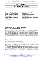
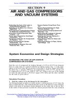
FIGURE 1 Shaft and 6-spoked bearing system hav-
ing three rotor masses. (Product Engineering.)
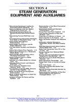
SECTION 22
BEARING DESIGN AND
SELECTION
Determining Stresses, Loading, Bending
Moments, and Spring Rate in Spoked
Bearing Supports 22.1
Hydrodynamic Equations for Bearing
Design Calculations 22.6
Graphic Computation of Bearing Loads
on Geared Shafts 22.13
Shaft Bearing Load Analysis Using Polar
Diagrams 22.17
Journal Bearing Frictional Horsepower
Loss During Operation 22.21
Journal Bearing Operation Analysis
22.22
Bearing Type Selection of a Known
Load 22.23
Shaft Bearing Length and Heat
Generation 22.28
Roller-Bearing Operating-Life Analysis
22.31
Roller-Bearing Capacity Requirements
22.32
Radial Load Rating for Rolling Bearings
22.32
Roller-Bearing Capacity and Reliability
22.34

Porous-Metal Bearing Capacity and
Friction 22.35
Hydrostatic Thrust Bearing Analysis
22.37
Hydrostatic Journal Bearing Analysis
22.39
Hydrostatic Multidirection Bearing
Analysis 22.42
Load Capacity of Gas Bearings 22.46
DETERMINING STRESSES, LOADING, BENDING
MOMENTS, AND SPRING RATE IN SPOKED
BEARING SUPPORTS
Spoked bearing supports are used in gas turbines, large air-cooling fans, electric-
motor casings slotted for air circulation, and a variety of other applications. For the
shaft and 6-spoked bearing system in Fig. 1 having three rotor masses and these
parameters and symbols,
Downloaded from Digital Engineering Library @ McGraw-Hill (www.digitalengineeringlibrary.com)
Copyright © 2006 The McGraw-Hill Companies. All rights reserved.
Any use is subject to the Terms of Use as given at the website.
Source: HANDBOOK OF MECHANICAL ENGINEERING CALCULATIONS
22.2 DESIGN ENGINEERING
SI values
P ϭ 10,000 lb (at either bearing)
4
I ϭ 25 in
S
4
I ϭ 0.3 in
R
2

A ϭ 7 in (for ring also)
6
E ϭ E ϭ 10 ϫ 10 psi
SR
L ϭ 10 in
R
ϭ 12 in
C
ϭ 0.40 in
R
(44,480 N)
(1040.6 cm
4
)
(12.5 cm
4
)
(45.2 cm
2
)
(68,900 MPa)
(25.4 cm)
(30.5 cm)
(8.9 cm)
(1.02 cm)
Symbols SI values
A ϭ spoke cross-section area, in
2
(cm
2

)
C
S
ϭ distance, neutral axis to extreme fiber (of spoke), in (cm)
C
R
ϭ distance, neutral axis to extreme fiber (of ring), in (cm)
E
R
, E
S
ϭ elasticity moduli (ring and spoke), psi (kPa)
R
R1
ϭ axial loading in inclined spokes, lb; (ϩ for upper two, Ϫ for lower
two)
(N)
F
R2
ϭ axial loading in vertical spokes, lb; (ϩ for top, Ϫ for bottom) (N)
F
T
ϭ tangential load at OD of inclined spokes, lb; (clockwise on left side,
counterclockwise on right side)
(N)
I
R
ϭ outer-ring moment of inertia about neutral axis pependicular to plane
of support, in
4

(cm
4
)
I
S
ϭ spoke moment of inertia about neutral axis perpendicular to plane of
support, in
4
(cm
4
)
k
ϭ spring rate with respect to outer shell, lb/in (N/cm)
L
ϭ spoke length, in (cm)
M
ϭ max bending moment (6-spoked support) in outer ring at OD of
vertical spokes, in-lb; (
ϩ at inner-fiber upper point and outer-fiber
lower point)
ϭ max bending moment at OD of all spokes in 4-spoked support
(Nm)
P
ϭ bearing radial-load, lb (N)
R
ϭ ring radius, in (cm)
T
ϭ axial loading in outer ring at OD of vertical spokes in 6-spoked
support; all spokes in 4-spoked support (
Ϫ at upper points, ϩ at

lower points)
lb (N)
ϩ denotes tension
Ϫ denotes compression
find (a) the maximum bending moment in the outer ring of the support, (b) the
axial loading in the outer ring, (c) the total stress in the outer ring at the top vertical
spoke, Fig. 2, (d) the total axial loading in one of the inclined spokes, (e) the
bending moment in the spoke at the hub, and (f) the spring rate of the spoked
bearing support. Use the free-body diagram, Fig. 3, to analyze this bearing support.
Calculation Procedure:
1. Find the maximum bending moment in the outer ring of the 6-spoke bearing
support
Use the relation
Downloaded from Digital Engineering Library @ McGraw-Hill (www.digitalengineeringlibrary.com)
Copyright © 2006 The McGraw-Hill Companies. All rights reserved.
Any use is subject to the Terms of Use as given at the website.
BEARING DESIGN AND SELECTION
BEARING DESIGN AND SELECTION 22.3
FIGURE 2 Typical 6-spoke bearing support having the mount
load at the top for an aircraft gas turbine; in a stationary plant, mount
load would be at the bottom of the support. (Product Engineering.)
3
IE
R
SS
ϭ abscissae parameter, Fig. 4
ͩͪͩͪͩͪ
ILE
RR
where the symbols are as shown above. Substituting, we find the parameter ϭ 144,

from:
3
25 12 1
ͩͪͩͪͩͪ
0.3 10 1
Using the M curve in Fig. 4 for a parameter value of 144 gives
100M
ϭ 1.45
PR
Solving for M,wehave
1.45 PR 1.45(10,000)(12)
M ϭϭ ϭ1740 in/lb (196.6 Nm)
100 100
2. Determine the axial loading in the outer ring at the outside diameter (OD)
Find T, the axial loading from Fig. 4 for the 144 parameter as
10T
ϭ 1.55
P
Substituting,
Downloaded from Digital Engineering Library @ McGraw-Hill (www.digitalengineeringlibrary.com)
Copyright © 2006 The McGraw-Hill Companies. All rights reserved.
Any use is subject to the Terms of Use as given at the website.
BEARING DESIGN AND SELECTION
22.4 DESIGN ENGINEERING
FIGURE 3 Free-body diagram for 6- and 4-spoke bearing
supports. (Product Engineering.)
1.55P (1.55)(10,000)
T ϭϭ ϭ1550 lb (6894 N)
10 10
3. Compute the total stress in the outer ring at the top vertical spoke

Use the relation
T (0.4) 1550
2
M(C /I ) ϩϭ1740 ϩϭ2320 ϩ 220 ϭ 2540 lb/in (17501 kPa)
RR
A (0.3) 7
4. Find the total axial loading in one of the inclined spokes
Using the F
R1
curve in Fig. 4 for the same parameter, 144,
10F 0.82 P (0.82)(10,000)
R1
ϭ 0.82 F ϭϭ ϭ820 lb (3647 N)
R1
P 10 10
Also,
10F (1.47)(P) (1.47)(10,000)
T
ϭ 1.47 F ϭϭ ϭ1470 lb (6539 N)
T
P 10 10
Downloaded from Digital Engineering Library @ McGraw-Hill (www.digitalengineeringlibrary.com)
Copyright © 2006 The McGraw-Hill Companies. All rights reserved.
Any use is subject to the Terms of Use as given at the website.
BEARING DESIGN AND SELECTION
BEARING DESIGN AND SELECTION 22.5
FIGURE 4 Six-spoke bearing-support parameter curves. (Product Engineering.)
5. Determine the bending moment in the spoke at the hub
The bending moment in the spoke at the hub is (F
T

)(L) ϭ (1470)(10) ϭ 14,700 in-
lb (1661 Nm)
ϭ M
S
.
Then, the total stress in this section is
CF
(3.5) 820
SR1
M ϩϭ(14,700) ϩ
ͩͪ
S
IA 25 7
S
2
ϭ 2060 ϩ 120 ϭ 2180 lb /in (15,020 kPa)
6. Find the spring rate of the spoked bearing support
For the 144 parameter,
3 6
kR (2850) IE (2850)(0.3)(10)(10 )
RR
ϭ 2850, whence k ϭ k ϭ
33
IE R (12)
RR
6
ϭ 4.93 ϫ 10 lb/in (8633 kN /cm)
Related Calculations. Figure 5 gives values for 4-spoke bearing supports. Use
it in the same way that Fig. 4 was used in this procedure.
With more jet aircraft being built, an increase in the use of aero-derivative gas

turbines in central-station and industrial power plants, wider use of air conditioning
throughout the world, and construction of larger and larger electric motors, the
Downloaded from Digital Engineering Library @ McGraw-Hill (www.digitalengineeringlibrary.com)
Copyright © 2006 The McGraw-Hill Companies. All rights reserved.
Any use is subject to the Terms of Use as given at the website.
BEARING DESIGN AND SELECTION
22.6 DESIGN ENGINEERING
FIGURE 5 Four-spoke bearing-support parameter curves. (Product Engineering.)
spoked bearing support is gaining greater attention. The procedure presented here
can be used for any of these applications, plus many related ones.
In calculations for spoked bearings the rings are assumed supported by sinuso-
idally varying tangential skin-shear reactions. Spokes are also assumed pinned to
the ring but rigidly attached to the hub.
This procedure is the work of Lawrence Berko, Supervising Design Engineer,
Walter Kide & Co., as reported in Product Engineering magazine. SI values were
added by the handbook editor.
HYDRODYNAMIC EQUATIONS FOR BEARING
DESIGN CALCULATIONS
Bearing design also requires a number of hydrodynamic formulas involving hy-
draulics, fluid flow, power, pressure head, torque, fluid viscosity, and fluid density.
Table 1 presents useful formulas for the hydrodynamic design of bearings in both
USCS and SI units.
Downloaded from Digital Engineering Library @ McGraw-Hill (www.digitalengineeringlibrary.com)
Copyright © 2006 The McGraw-Hill Companies. All rights reserved.
Any use is subject to the Terms of Use as given at the website.
BEARING DESIGN AND SELECTION
22.7
TABLE 1 Hydrodynamic Equations for Bearing Design
Name Unit Symbol Formula or value System
Mass Slugs M

2
lb ϫ s
ft
USCS
Kilogram mass Metric slug M
2
kg ϫ s
m
SI
Gram mass
2
dyn ϫ s
cm
M
2
dyn ϫ s
cm
SI
Gravitational constant
ft
2
s
g 32.174 (in London) USCS
m
2
s
g 9.807 (in Paris) SI
Force dyn P
1
g

981
SI
Poundal P
1
lb
32.174
USCS
Pressure head ft H For water, 1 ft equals 0.433 lb / in
2
or 62.335
lb/ft
2
USCS
Rated work hp N 550 ft ⅐ lb / s or 33,000 ft ⅐ lb / min USCS
hp N
3
ft head ϫ sp gr
ϫ or
s 8.8
USCS
gal head
ϫ sp gr
ϫ
min 3960
hp N
3
ft lb 1
ϫϫ or
2
min ft 33,000

USCS
gal lb 1
ϫϫ
2
min in 1714
Downloaded from Digital Engineering Library @ McGraw-Hill (www.digitalengineeringlibrary.com)
Copyright © 2006 The McGraw-Hill Companies. All rights reserved.
Any use is subject to the Terms of Use as given at the website.
BEARING DESIGN AND SELECTION
22.8
TABLE 1 (Continued )
Name Unit Symbol Formula or value System
Torque lb ⅐ ft T
hp
ϫ 33,000 5250
ϭ
rpm ϫ 2
␲
rpm
USCS
Density
Mass
Unit volume
␳
2
lb s slugs
ϫϭ
33
ft ft ft
SI

Mass
Unit volume
␳
2
gs
ϫ
3
cm cm
Absolute viscosity in USCS units
Mass
Length ϫ Time
␮
slugs lb ⅐ s
ϭ
2
ft ⅐ sft
USCS
1 unit of
ϭ 178.69 P
slugs
ft ⅐ s
␮
A
lb ⅐ min
ϭ 4,136,000 P
2
in
poundal
⅐ s
ϭ 14.88 P

2
ft
Absolute viscosity in SI units P
1 dyn
⅐ s
2
cm
SI
cP Z
1
P
100
g
⅐ s
2
cm
981 P
Downloaded from Digital Engineering Library @ McGraw-Hill (www.digitalengineeringlibrary.com)
Copyright © 2006 The McGraw-Hill Companies. All rights reserved.
Any use is subject to the Terms of Use as given at the website.
BEARING DESIGN AND SELECTION
22.9
Kinematic viscosity
Area
Time
␯
␮
absolute viscosity
␯
ϭϭ

␳
density
USCS and SI
St,
2
cm
s
1P
Density
SI
cSt
1
St
100
Saybolt universal seconds V For conversion of SUS units into centistokes SI
When SUS
Ϲ 100 cSt ϭ 0.226 SUS. Ϫ 195 /
SUS.
When SUS.
ϭ 100 cSt ϭ 0.220 SUS. Ϫ 135 /
SUS.
Specific viscosity Dimensionless Ratio of absolute viscosity of any fluid to that
of water at a temperature of 20
ЊC
Absolute value
Viscosity of water at a
temperature of 20
ЊC
cP ZZ
ϭ 1cP SI

Fluidity
Length
ϫ time
Mass
␾␾
ϭ inverse value of absolute viscosity
1
␮
SI and USCS
Reynolds number Dimensionless N
R
␳
vd vd
N ϭϭ
R
␮␯
v ϭ velocity of fluid
␳
ϭ density
d
ϭ pipe diameter
␮
ϭ absolute viscosity
␯
ϭ kinematic viscosity
Absolute value
Downloaded from Digital Engineering Library @ McGraw-Hill (www.digitalengineeringlibrary.com)
Copyright © 2006 The McGraw-Hill Companies. All rights reserved.
Any use is subject to the Terms of Use as given at the website.
BEARING DESIGN AND SELECTION

22.10
TABLE 1 (Continued )
Name Unit Symbol Formula or value System
Critical Reynolds number for
pipe flow
Dimensionless N
e
N
e
ϭ 2320 ϭ Reynolds number which
represents the separation point between
laminar and turbulent flow
Absolute value
For N
R
Ͼ 2320, turbulent flow
For N
R
Ͻ 2320 laminar flow
From N
R
ϭ 1920 to 4000, instability flow
Friction loss formula for pipe
flow
ft or m H
ƒ
H
ƒ
ϭ ƒ ϫ
2

1 v
ϫ
d 2g
SI and USCS
v ϭ velocity, ft / s or m / s
d
ϭ pipe dia., ft or m
l
ϭ pipe length, ft or m
22
g ϭ gravity constant, ft / s or m / s
ƒ
ϭ flow coefficient
Flow coefficient for laminar
(viscous) flow
Dimensionless ƒ 64
ƒ ϭ
N
R
Absolute value
Grade or roughness of pipe is immaterial
Flow coefficient for clean cast-
iron pipe—circular section
Dimensionless ƒ 0.214
ƒ ϭ turbulent flow
5
N
͙
R
64

ƒ ϭ laminar flow
N
R
Absolute value
Flow coefficient for very smooth
pipe, circular section
Dimensionless ƒ 0.316
ƒ ϭ turbulent flow
4
N
͙
R
64
ƒ ϭ laminar flow
N
R
Absolute value
Downloaded from Digital Engineering Library @ McGraw-Hill (www.digitalengineeringlibrary.com)
Copyright © 2006 The McGraw-Hill Companies. All rights reserved.
Any use is subject to the Terms of Use as given at the website.
BEARING DESIGN AND SELECTION
22.11
Flow coefficient for maximum
degree of roughness
Dimensionless ƒ 0.316
ƒ ϭ
4
N
͙
R

ϭ 0.054 turbulent flow
64
ƒ ϭ laminar flow
N
R
Absolute value
Reynolds number for water of
20
ЊC temperature
Dimensionless N
R
N ϭ 100vd
R
v ϭ velocity, cm / s
d
ϭ pipe dia., cm
Absolute value
Bearing constant (Sommerfeld
variable)
Dimensionless S
2
D
␮
n
S ϭ
ͩͪ
cp
D
ϭ bearing diameter
c

ϭ bearing clearance
ϭ bearing diameter
Ϫ shaft diameter
␮
ϭ absolute viscosity
p
ϭ unit pressure
n
ϭ revolutions per time unit
Absolute value
Downloaded from Digital Engineering Library @ McGraw-Hill (www.digitalengineeringlibrary.com)
Copyright © 2006 The McGraw-Hill Companies. All rights reserved.
Any use is subject to the Terms of Use as given at the website.
BEARING DESIGN AND SELECTION
22.12
TABLE 1 (Continued )
Name Unit Symbol Formula or value System
Example Dimensionless S
␮
n
S ϭ 1,000,000 ϫ
p
Absolute value
Find Sommerfeld variable for D/
C
ϭ 1000
1,000,000Zn
ϭ
4,136,000 ϫ 100 ϫ p
␮

ϭ absolute viscosity,
A
2
lb ⅐ min/in
n
ϭ rpm
2
p ϭ lb/in
Z
ϭ absolute viscosity, cSt
For
ϭ 36,
Zn
p
S
ϭ 0.00242 ϫ 36 ϭ 0.087
Note: Burwell’s charts show maximum
allowable pressure at s
ϭ 0.267 but
reasonably high pressure and minimum
coefficient of friction at range
S
ϭ 0.080 to S ϭ 0.50
(See ASME Transactions 1942, p. 457.)
Bearing constant Dimensionless S
z
Zn
S ϭ
z
p

Z
ϭ absolute viscosity, cP
n
ϭ rpm
2
p ϭ unit pressure, lb / in
Absolute value
Downloaded from Digital Engineering Library @ McGraw-Hill (www.digitalengineeringlibrary.com)
Copyright © 2006 The McGraw-Hill Companies. All rights reserved.
Any use is subject to the Terms of Use as given at the website.
BEARING DESIGN AND SELECTION
BEARING DESIGN AND SELECTION 22.13
FIGURE 6 Gear loads on a typical gear. (Product Engi-
neering.)
GRAPHIC COMPUTATION OF BEARING LOADS
ON GEARED SHAFTS
Geared shafts having loads and reactions as shown in Fig. 6 are arranged as shown
in Fig. 7. The physical characteristics of the gears are:
Pitch dia. of gears Moment arm
A ϭ 2 in (5.08 cm) a ϭ 1.50 in (3.81 cm)
B
ϭ 1.50 in (3.81 cm) b ϭ 3.50 in (8.89 cm)
C
ϭ 4.00 in (10.16 cm) c ϭ 5.00 in (12.7 cm)
Driver
ϭ 1.75 in (4.45 cm) d ϭ 7.00 in (17.78 cm)
Angle, deg
alpha
ϭ 55
beta

ϭ 48
tau
ϭ 45
Torque on driver
ϭ 100 lb/in (11.3 Nm)
Torque delivered by A
ϭ 40 percent of torque on center shaft
Torque delivered by B
ϭ 60 percent on center shaft
Pressure angle of all gears,
␾
ϭ 20 deg
Determine the bearing loads resulting from gear action using the total force directly.
Use a combined numerical and graphical solution.
Calculation Procedure:
1. Find the load on each gear in the set
The tangential forces, F
T
on the driver, Fig. 6, is F
T
ϭ 2T / D, where T ϭ torque
transmitted by the gear, lb /in (Nm); D
ϭ gear pitch diameter, in (cm). Substituting
Downloaded from Digital Engineering Library @ McGraw-Hill (www.digitalengineeringlibrary.com)
Copyright © 2006 The McGraw-Hill Companies. All rights reserved.
Any use is subject to the Terms of Use as given at the website.
BEARING DESIGN AND SELECTION
22.14
FIGURE 7 Typical gear set for which the bearing loads are computed. (Product Engineering.)
Downloaded from Digital Engineering Library @ McGraw-Hill (www.digitalengineeringlibrary.com)

Copyright © 2006 The McGraw-Hill Companies. All rights reserved.
Any use is subject to the Terms of Use as given at the website.
BEARING DESIGN AND SELECTION
BEARING DESIGN AND SELECTION 22.15
SI Values
1148 lb-in. (129.7 Nm)
608 lb-in. (68.7 Nm)
621 lb-in. (70.2 Nm)
145.5 lb-in. (16.4 Nm)
FIGURE 8 Couple vector diagram for the gear set in Fig. 7 (Product Engineering.)
TABLE 2
Bearing Loads on Geared Shafts
Gear or
bearing
Distance from
X, in (cm) Force lb (N)
Couple lb / inЊ
(NmЊ)
Angular
position
A Ϫ1.5 (Ϫ3.81) 97 (431.5) Ϫ145.5 (Ϫ16.4) 115
I0P
I
00
B 3.5 195 (867.4 N) 621 (70.2) 202
C 5.00 121.5 (68.7) 608 (68.7) 165
II 7.00 P
II
7 P
II

⌬
with the given torque on the driver of 100 lb / in (11.3 Nm), we have, F
T
ϭ
2(100)/ 1.75 ϭ 114 lb (508 N). Then, the torque on the center shaft ϭ D(F
T
) ϭ
2(114) ϭ 228 lb /in (25.8 Nm).
The gear loads are computed from F
A
ϭ (percent torque on shaft)(2)(torque on
center shaft, lb / in)(sec of pressure angle on the gear)/ D , where F
A
ϭ gear load, lb
(N), on gear A, Fig. 7. Substituting using the given and computed values, F
A
ϭ
0.4 (2)(228)(sec 20Њ)/2 ϭ 97 lb (431.5 N). Likewise, for gear B using a similar
relation, F
B
ϭ 0.6 (2)(228)(sec 20Њ)/1.5 ϭ 195 lb (867.4 N). Further, F
C
, for gear
C
ϭ 114 (sec 20Њ) ϭ 121.5 lb (540 N).
2. Collect the needed data to prepare the graphical solution
Assemble the data as shown in Table 2.
3. Prepare the couple diagram, Fig. 8
When all the data are collected, draw the couple diagram, Fig. 8. When drawing
this couple diagram it is important to note that: (a) Vectors representing negative

couples are drawn in the same direction but in opposite sense to the forces causing
them; (b) The direction of the closing should be such as to make the sum of all
Downloaded from Digital Engineering Library @ McGraw-Hill (www.digitalengineeringlibrary.com)
Copyright © 2006 The McGraw-Hill Companies. All rights reserved.
Any use is subject to the Terms of Use as given at the website.
BEARING DESIGN AND SELECTION
22.16 DESIGN ENGINEERING
SI Values
164 lb (729.5 N)
121 lb (538.2 N)
195 lb (867.4 N)
184 lb (818.4 N)
97 lb (431.5 N)
FIGURE 9 Force vector diagram for the gear set in Fig. 7. (Product Engineering.)
couples equal to zero. Thus, the direction of P
II
is the direction of bearing reaction.
The bearing load has the same direction but is of opposite sense.
In Fig. 8, the vector P
II
measures 1149 lb /in (129.7 Nm) to scale. Therefore,
the reaction on the bearing II is P
II
ϭ 1148/ 7 ϭ 164 lb (729.7 N) at 11.5Њ.
4. Construct the force vector diagram
The value of P
II
found in step 3 is now used to construct the force vector diagram
of forces acting at point X, Fig. 9. Drawing the closing line gives the value and
direction of the reaction on bearing I. The force vectors are drawn in the usual way

in their respective directions and sense. Then, the loading on bearing I is P
I
ϭ 184
lb (818.4 N) at 27.5
Њ.
Related Calculations. The principles used in this procedure to obtain loads on
bearings supporting the center shaft in Fig. 7 can be applied to obtain loads on
bearings carrying shafts with any number of gears. It is limited, however, to those
cases which are statistically determinate.
Bending-moment and shear diagrams can now be constructed since the magni-
tude and direction of all forces acting on the shaft are known. To calculate the
bearing loads resulting from gear action, both the magnitude and direction of the
tooth reaction must be known. This reaction is the force at the pitch circle exerted
by the tooth in the direction perpendicular to, and away from the tooth surface.
Thus, the tooth reaction of a gear is always in the same general direction as its
motion.
Most techniques for evaluating bearing loads separate the total force acting on
the gear into tangential and separating components. This tends to complicate the
solution. The method given in this procedure uses the total force directly.
Since a force can be replaced by an equal force acting at a different point, plus
a couple, the total gear force can be considered as acting at the intersection of the
shaft centerline and a line passing through the mid-face of the gear, if the appro-
Downloaded from Digital Engineering Library @ McGraw-Hill (www.digitalengineeringlibrary.com)
Copyright © 2006 The McGraw-Hill Companies. All rights reserved.
Any use is subject to the Terms of Use as given at the website.
BEARING DESIGN AND SELECTION
BEARING DESIGN AND SELECTION 22.17
SI Values
1600 lb-in. (180.8 Nm)
1.625 in. (4.128 cm

8 in. (20.3 cm)
1.00 in. (2.54 cm)
3.00 in. (7.62 cm)
4.00 in. (10.16 cm)
3.50 in. (8.89 cm)
2100 lb (9341 N)
1970 lb (8763 N)
718 (3194 N)
FIGURE 10 Sheave drive having bearing side loads. (Product Engineering.)
priate couple is included. For example, in Fig. 7, the total force on gear B is
equivalent to a force F
B
applied at point X plus the couple b ϫ F
B
. In establishing
the couples for the other gears, a sign convention must be adopted to distinguish
clockwise and counterclockwise moments.
If a vector diagram is now drawn for all couples acting on the shaft, the closing
line will be equal (to scale) to the couple resulting from the reaction at bearing II.
Knowing the distance between the two bearings, the load on bearing II can be
found, the direction being the same as that of the couple caused by it.
The load on bearing I is found in the same manner by drawing force vector
diagram for all the forces acting at X, including the load on bearing II found from
the couple diagram.
This procedure is the work of Zbigniew Jania, Project Engineer, Ford Motor
Company, as reported in Product Engineering. SI values were added by the hand-
book editor.
SHAFT BEARING LOAD ANALYSIS USING POLAR
DIAGRAMS
Determine the allowable directional side loads in the sheave drive in Fig. 10 if the

maximum permissible radial load in bearing A is 2100 lb (9341 N) and 3750 lb
(16,680 N) in bearing B when the maximum torque transmitted by the pinion is
Downloaded from Digital Engineering Library @ McGraw-Hill (www.digitalengineeringlibrary.com)
Copyright © 2006 The McGraw-Hill Companies. All rights reserved.
Any use is subject to the Terms of Use as given at the website.
BEARING DESIGN AND SELECTION
22.18 DESIGN ENGINEERING
SI Values
1575 lb (7006 N)
525 lb (2335 N)
1 in. (2.54 cm)
3 in. (7.62 cm)
2100 lb (9341 N)
FIGURE 11 Load diagram for sheave drive shaft. (Product Engineering.)
1600 lb /in (181 Nm). The tangential and separating forces at the point of tooth
contact are 1970 lb (8763 N) and 718 lb (3194 N) respectively. Use numerical and
graphical analysis methods.
Calculation Procedure:
1. Construct a vector diagram to determine the side forces on the bearings
Draw the vector diagram in Fig. 10 to combine the tangential and separating forces
of 1970 lb (8763 N) and 718 lb (3195 N) vectorially to give a resultant R of 2100
lb (9341 N). This resultant, R, can be replaced by a parallel force, R
Ј, of equal
magnitude at the shaft centerline and a moment of 1970
ϫ 4inϭ 7880 lb/in (890
Nm) in a plane normal to the shaft centerline.
Construct a load diagram, of the shaft, Fig. 11. Taking moments, we find that
the resultant loads at the bearings are: Bearing A
ϭ 1575 lb (7006 N); Bearing B
ϭ 525 lb (2335 N). Next, each bearing load condition must be treated separately.

2. Use the fictitious-force approach to find the bearing load conditions
The key to the solution is to replace R
Ј with fictitious forces in the plane of the
output sheave, Fig. 10, of such magnitudes that the bearing loads are unchanged.
Figures 12a and 12b show the procedure and the necessary forces with their
directions of application. These fictitious forces, if plotted to some convenient scale
on polar coordinate paper with the leading edge at the origin, will represent the
bearing loads resulting from gear action.
If the side load is applied in the same direction as fictitious force R
Ј
A
, it will be
limited by the allowable bearing capacity of bearing A. Since the maximum per-
missible radial load is given as 2100 lb (9341 N) by the bearing manufacturer, the
resultant radial force, R
Ј
A
, acting in the plane of the output sheave must not exceed
2400 lb (10,675 N), since from Fig. 12a: (1575
ϩ 525)4 ϭ (1800 ϩ 600)3.5. Of
this 2400 lb (10,675 N), the fictitious force of 1800 lb (8006 N) must be considered
a definite component. The actual applied load would then be limited to 600 lb
(2669 N) (
ϭ 2400 Ϫ 1800), in the direction of RЈ
A
.
Downloaded from Digital Engineering Library @ McGraw-Hill (www.digitalengineeringlibrary.com)
Copyright © 2006 The McGraw-Hill Companies. All rights reserved.
Any use is subject to the Terms of Use as given at the website.
BEARING DESIGN AND SELECTION

BEARING DESIGN AND SELECTION 22.19
SI Values
1575 lb (7006 N)
1800 lb (8006 N)
525 lb (2335 N)
280 lb (1245 N)
4 in. (10.16 cm)
3.5 in. (8.89 cm)
FIGURE 12 Load diagram for sheave dive shaft using fictitious forces. (Product Engineering.)
If applied in the opposite direction, the limiting side load becomes 4200 lb
(18,682 N) (
ϭ 2400 ϩ 1800), since it acts to nullify rather than to complement the
fictitious force in producing bearing load. Recalling the principles of polar dia-
grams, it is now apparent that a circle of 2400 lb (10,675 N) equivalent radius,
R
Ј
AL
, would result in a polar diagram, Fig. 13, of permissible side loading for the
design life of Bearing A. The validity of this solution and operation is understood
by noting that the equivalent radius is always the resultant of the fictitious force,
R
Ј
A
and the rotating vector which represents the applied side load.
3. Analyze the other bearing in the system using a similar procedure
We will repeat the same procedure for Bearing B, Fig. 10, which has a design life
(either assumed or given by the manufacturer) compatible with the 3750 lb (16,680
N) maximum rated load. When superimposed on one another, these diagrams give
a confined realm of loading (k-l-m-n), Fig. 13.
Using the chosen scale, it is now possible to conveniently measure load limi-

tations in any direction. When dividing the torque transmitted at the sheave, namely
7880 lb/in (890 Nm), Fig. 10, by any maximum indicated side load, the corre-
sponding minimum sheave diameter is obtained.
4. Analyze the shaft stresses based on desired bearing life
Now that the side-load limitations, based on desired bearing life, have been estab-
lished, the imposed shaft stresses can be analyzed. Consider the stress to be critical
under Bearing B. For safe loading limit, the maximum equivalent bending will be
taken as 7200 lb/in (814 Nm). The equation for combined bending and torsion is:
22
11
M ϭ ⁄
2
M ϩ ⁄
2
͙M ϩ T
c
Substituting known quantities,
Downloaded from Digital Engineering Library @ McGraw-Hill (www.digitalengineeringlibrary.com)
Copyright © 2006 The McGraw-Hill Companies. All rights reserved.
Any use is subject to the Terms of Use as given at the website.
BEARING DESIGN AND SELECTION
22.20 DESIGN ENGINEERING
SI Values
2400 lb (10,675 N)
280 lb (1245 N)
1800 lb (8006 N)
(2.54 cm = 5338 N)
FIGURE 13 Polar diagram of sheave drive showing side forces. (Product Engineering.)
Downloaded from Digital Engineering Library @ McGraw-Hill (www.digitalengineeringlibrary.com)
Copyright © 2006 The McGraw-Hill Companies. All rights reserved.

Any use is subject to the Terms of Use as given at the website.
BEARING DESIGN AND SELECTION
BEARING DESIGN AND SELECTION 22.21
FIGURE 14 Operating condition of a loaded journal bearing.
22
11
7,200 ϭ ⁄
2
M ϩ ⁄
2
͙M ϩ 7,880
The maximum allowable bending moment is then 5000 lb/in (565 Nm). At the
specified distance of overhang, the side load, Q, caused by chain or belt pull is
therefore limited by the shaft strength of 1430 lb (6361 N) in any direction. This
limitation is shown on the polar diagram, Fig. 13, by a circle with its center at the
origin and a radius equivalent to 1430 lb (6361 N). Study of the polar diagram,
Fig. 10, shows that Bearing B is no longer a limiting factor since it completely
encloses the now smaller region of safe loading.
Related Calculations. When applying belt and chain drives to geared power
transmitting devices, excessive side loads are a frequent source of trouble in the
bearings. Improper selection of sheaves and arrangement of connections can result
in poor bearing life and early shaft breakage. A thorough analysis of bearing loads
and shaft stresses is necessary if these troubles are to be avoided.
Use of polar diagrams provides a unique method of determining the maximum
permissible side loading and the minimum size sheaves on an overhung shaft where
gear loading is present. This type of analysis gives a graphical representation of
limiting side loads with relation to their corresponding directions of pull. In essence
it becomes a permanent data sheet for an individually designed unit to which future
reference is readily available. The approach given here is valid for geared drives in
factories, waterworks installations, marine applications, air conditioning and ven-

tilation, etc., wherever an overhung shaft is used.
This procedure is the work of Richard J. Derks, Assistant Professor of Mechan-
ical Engineering, University of Notre Dame, formerly Design Engineer, Twin Disc
Clutch Company, as reported in Product Engineering.
JOURNAL BEARING FRICTIONAL HORSEPOWER
LOSS DURING OPERATION
An 8-in (20.3-cm) diameter journal bearing is designed for 140-degree optimum
oil-film pressure distribution, Fig. 14, when the journal length is 9 in (22.9 cm),
shaft rotative speed is 1800 rpm, and the total load is 20,000 lb (9080 kg). What
is the frictional horsepower loss when this journal bearing operates under stated
conditions with oil of optimum viscosity?
Downloaded from Digital Engineering Library @ McGraw-Hill (www.digitalengineeringlibrary.com)
Copyright © 2006 The McGraw-Hill Companies. All rights reserved.
Any use is subject to the Terms of Use as given at the website.
BEARING DESIGN AND SELECTION
22.22 DESIGN ENGINEERING
Calculation Procedure:
1. Find the journal rubbing speed
The rubbing speed of a journal bearing is given by V
r
ϭ
␲
(D)(rpm), where D ϭ
journal diameter, ft (m). Substituting, V
r
ϭ 3.1416(8.12)(1800) ϭ 3770 ft /min
(1149 m / min).
2. Compute the rubbing surface area
The rubbing surface area of a journal bearing, A
r

ϭ (d/2)(
␣
)(
␲
)(L), where d ϭ
bearing diameter, in;
␣
ϭ optimum bearing angle, degrees; L ϭ bearing length, in.
Substituting, A
r
ϭ (8/ 2)(140/ 180)(
␲
)(9) ϭ 87.96 in
2
(567.5 cm
2
).
3. Calculate the bearing pressure
With a total load of 20,000 lb (9080 kg), the bearing pressure ϭ total load/ bearing
rubbing surface area, or 20,000/ 87.96
ϭ 227.4 lb /in
2
(1567 kPa).
4. Find the frictional horsepower (kW) loss
Use the relation ƒ
hl
ϭ
␮
(P)(V
r

)/ 33,000, where ƒ
hl
ϭ frictional hp (kW) loss;
␮
ϭ
coefficient of friction for the journal bearing; P ϭ total load on the bearing, lb (kg);
V
r
ϭ rubbing speed, ft /min.
Using standard engineering handbooks, the coefficient of friction can be found
to be 0.002 for a journal bearing having the computed rubbing speed and the given
bearing pressure. Substituting,
ƒ
ϭ (0.002)(20,000)(377)/33,000 ϭ 4.569 hp (3.4 kW).
hl
Related Calculations. Use this general procedure to find the frictional power
loss in journal bearings serving motors, engines, pumps, compressors, and similar
equipment. Data on the coefficient of friction is available in standard handbooks.
Figure 15 shows a typical plot of the coefficient of friction for journal bearings.
The coefficient of friction chose for a well-designed journal bearing is that for full
fluid film lubrication.
JOURNAL BEARING OPERATION ANALYSIS
A 2.5-in (6.36-cm) diameter journal bearing is subjected to a load of 1000 lb (454
kg) while the shaft it supports is rotating at 200 rpm. If the coefficient of friction
is 0.02 and L/D
ϭ 3.0, find (a) bearing projected area, (b) pressure on bearing, (c)
total work, (d) work of friction, (e) total heat generated, and (f) heat generated per
minute per unit area.
Calculation Procedure:
1. Determine the bearing dimensions and projected area

The length/ diameter ratio, L/ D
ϭ 3.0; hence L ϭ 3D ϭ 3 ϫ 2.25 ϭ 6.75 in (17.15
cm). (a) Then the projected area
ϭ L ϫ D ϭ 6.75 ϫ 2.5 ϭ 15.19 in
2
(97.99 cm
2
).
2. Find the pressure on the bearing and the total work
(b) The pressure on the bearing
ϭ total load on bearing, P lb/(projected area, in
2
)
ϭ 1000 /15.19 ϭ 65.8 lb / in
2
(453.6 kPa). (c) The total friction work transmitted
Downloaded from Digital Engineering Library @ McGraw-Hill (www.digitalengineeringlibrary.com)
Copyright © 2006 The McGraw-Hill Companies. All rights reserved.
Any use is subject to the Terms of Use as given at the website.
BEARING DESIGN AND SELECTION
BEARING DESIGN AND SELECTION 22.23
FIGURE 15 Various zones of possible lubrication for a journal bearing.
by the bearing, W ϭ friction factor (P)(
␲
)(bearing diameter, in /12 in/ft)(rpm).
Substituting, W
ϭ 0.02(1000)(
␲
)(2.25/ 12)(200) ϭ 2356 ft-lb/ min (53.2 W).
3. Compute the work of friction and total heat generated

(d) The work of friction, w
ϭ W / LD, where the symbols are as defined earlier.
Substituting, w
ϭ 2356 /15.19 ϭ 155.1 ft-lb / min (3.5 W). (e) The total heat gen-
erated
ϭ Q ϭ W /778 ϭ 155.1 /778 ϭ 3.03 Btu/ min (3.19 kJ/ min).
4. Find the heat generated per unit area
The heat generated per unit area, q
ϭ w/ 778 ϭ 155.1/ 778 ϭ 0.199 Btu/ in
2
min
(0.0325 kJ / cm
2
min).
Related Calculations. This procedure shows that the analysis of journal bear-
ings is a simple task requiring knowledge only of the physical dimensions or ratios
of the bearing, the coefficient of friction and the shaft rpm. Using these data, any
journal bearing can be designed for the mechanical requirements of the machine or
structure.
BEARING-TYPE SELECTION FOR A KNOWN
LOAD
Choose a suitable bearing for a 3-in (7.6-cm) diameter 100-r/min shaft carrying a
total radial load of 12,000 lb (53,379 N). A reasonable degree of shaft misalignment
must be allowed by the bearing. Quiet operation of the shaft is desired. Lubrication
will be intermittent.
Downloaded from Digital Engineering Library @ McGraw-Hill (www.digitalengineeringlibrary.com)
Copyright © 2006 The McGraw-Hill Companies. All rights reserved.
Any use is subject to the Terms of Use as given at the website.
BEARING DESIGN AND SELECTION
22.24 DESIGN ENGINEERING

Calculation Procedure:
1. Analyze the desired characteristics of the bearing
Two major types of bearings are available to the designer, rolling and sliding.
Rolling bearings are of two types, ball and roller. Sliding bearings are also of two
types, journal for radial loads and thrust for axial loads only or for combined axial
and radial loads. Table 3 shows the principal characteristics of rolling and sliding
bearings. Based on the data in Table 3, a sliding bearing would be suitable for this
application because it has a fair misalignment tolerance and a quiet noise level.
Both factors are key considerations in the bearing choice.
2. Choose the bearing materials
Table 4 shows that a porous-bronze bearing, suitable for intermittent lubrication,
can carry a maximum pressure load of 4000 lb/in
2
(27,580.0 kPa) at a maximum
shaft speed of 1500 ft / min (7.62 m/ s). By using the relation l
ϭ L /(Pd), where l
ϭ bearing length, in, L ϭ load, lb, d ϭ shaft diameter, in, the required length of
this sleeve bearing is l
ϭ L/(Pd) ϭ 12,000/ [(4000)(3)] ϭ 1 in (2.5 cm).
Compute the shaft surface speed V ft/min from V ϭ
␲
dR/12, where d ϭ shaft
diameter, in; R
ϭ shaft rpm. Thus, V ϭ
␲
(3)(100)/ 12 ϭ 78.4 ft /min (0.4 m /s).
With the shaft speed known, the PV, or pressure-velocity, value of the bearing
can be computed. For this bearing, with an operating pressure of 4000 lb / in
2
(27,580.0 kPa), PV ϭ 4000 ϫ 78.4 ϭ 313,600 (lb / in

2
) (ft/min) (10,984.3 kPa ⅐ m
/s). This is considerably in excess of the PV limit of 50,000 (lb/ in
2
) (ft/min)
(1751.3 kPa
⅐ m/ s) listed in Table 4. To come within the recommended PV limit,
the operating pressure of the bearing must be reduced.
Assume an operating pressure of 600 lb /in
2
(4137.0 kPa). Then l ϭ L /(Pd) ϭ
12,000/ [(600)(3)] ϭ 6.67 in (16.9 cm), say 7 in (17.8 cm). The PV value of the
bearing then is (600)(78.4) ϭ 47,000 (lb/ in
2
) (ft/min) (1646.3 kPa ⅐ m/s). This is
a satisfactory value for a porous-bronze bearing because the recommend limit is
50,000 (lb / in
2
) (ft/min) (1751.3 kPa ⅐ m / s).
3. Check the selected bearing size
The sliding bearing chosen will have a diameter somewhat in excess of 3 in (7.6
cm) and a length of 7 in (17.8 cm). If this length is too great to fit in the allowable
space, another bearing material will have to be studied, by using the same proce-
dure. Figure 16 shows the space occupied by rolling and sliding bearings of various
types.
Table 5 shows the load-carrying capacity and maximum operating temperature
for oil-film journal sliding bearings that are regularly lubricated. These bearings are
termed full film because they receive a supply of lubricant at regular intervals.
Surface speeds of 20,000 to 25,000 ft/ min (101.6 to 127.0 m/ s) are common for
industrial machines fitted with these bearings. This corresponds closely to the sur-

face speed for ball and roller bearings.
4. Evaluate oil-film bearings
Oil-film sliding bearings are chosen by the method of the next calculation proce-
dure. The bearing size is made large enough that the maximum operating temper-
ature listed in Table 5 is not exceeded. Table 6 lists typical design load limits for
oil-film bearings in various services. Figure 17 shows the typical temperature limits
for rolling and sliding bearings made of various materials.
Downloaded from Digital Engineering Library @ McGraw-Hill (www.digitalengineeringlibrary.com)
Copyright © 2006 The McGraw-Hill Companies. All rights reserved.
Any use is subject to the Terms of Use as given at the website.
BEARING DESIGN AND SELECTION
BEARING DESIGN AND SELECTION 22.25
TABLE 3 Key Characteristics of Rolling and Sliding Bearings*
5. Evaluate rolling bearings
Rolling bearings have lower starting friction (coefficient of friction ƒ
ϭ 0.002 to
0.005) than sliding bearings (ƒ
ϭ 0.15 to 0.30). Thus, the rolling bearings is pre-
ferred for applications requiring low staring torque [integral-horsepower electric
motors up to 500 hp (372.9 kW), jet engines, etc.]. By pumping oil into a sliding
bearing, its starting coefficient of friction can be reduced to nearly zero. This ar-
rangement is used in large electric generators and certain mill machines.
Downloaded from Digital Engineering Library @ McGraw-Hill (www.digitalengineeringlibrary.com)
Copyright © 2006 The McGraw-Hill Companies. All rights reserved.
Any use is subject to the Terms of Use as given at the website.
BEARING DESIGN AND SELECTION