Handbook of Mechanical Engineering Calculations ar Episode 2 Part 4 docx

24.1
SECTION 24
MECHANICAL AND ELECTRICAL
BRAKES
Brake Selection for a Known Load 24.1
Mechanical Brake Surface Area and
Cooling Time 24.3
Band Brake Heat Generation,
Temperature Rise, and Required
Area 24.6
Designing a Brake and Its Associated
Mechanisms 24.8
Internal Shoe Brake Forces and Torque
Capacity 24.15
Analyzing Failsafe Brakes for
Machinery 24.17
BRAKE SELECTION FOR A KNOWN LOAD
Choose a suitable brake to stop a 50-hp (37.3-kW) motor automatically when power
is cut off. The motor must be brought to rest within 40 s after power is shut off.
The load inertia, including the brake rotating member, will be about 200 lb
⅐ ft
2
(82.7 N ⅐ m
2
); the shaft being braked turns at 1800 r/min. How many revolutions
will the shaft turn before stopping? How much heat must the brake dissipate? The
brake operates once per minute.
Calculation Procedure:
1. Choose the type of brake to use
Table 1 shows that a shoe-type electric brake is probably the best choice for stop-
ping a load when the braking force must be applied automatically. The only other

possible choice—the eddy-current brake—is generally used for larger loads than
this brake will handle.
2. Compute the average brake torque required to stop the load
Use the relation T
a
ϭ Wk
2
n/(308t), where T
a
ϭ average torque required to stop the
load, lb
⅐ ft; Wk
2
ϭ load inertia, including brake rotating member, lb ⅐ ft
2
, n ϭ shaft
speed prior to braking, r / min; t
ϭ required or desired stopping time, s. For this
brake, T
a
ϭ (200)(1800)/[308(40)] ϭ 29.2 lb ⅐ ft, or 351 lb ⅐ in (39.7 N ⅐ m).
3. Apply a service factor to the average torque
A service factor varying from 1.0 to 4.0 is usually applied to the average torque
to ensure that the brake is of sufficient size for the load. Applying a service factor
of 1.5 for this brake yields the required capacity
ϭ 1.5(351) ϭ 526 in ⅐ lb (59.4
N
⅐ m).
Downloaded from Digital Engineering Library @ McGraw-Hill (www.digitalengineeringlibrary.com)
Copyright © 2006 The McGraw-Hill Companies. All rights reserved.

Any use is subject to the Terms of Use as given at the website.
Source: HANDBOOK OF MECHANICAL ENGINEERING CALCULATIONS
24.2 DESIGN ENGINEERING
TABLE 1 Mechanical and Electrical Brake Characteristics
4. Choose the brake size
Use an engineering data sheet from the selected manufacturer to choose the brake
size. Thus, one manufacturer’s data show that a 16-in (40.6-cm) diameter brake
will adequately handle the load.
5. Compute the revolutions prior to stopping
Use the relation R
s
ϭ tn/120, where R ϭ number of revolutions prior to stopping;
other symbols as before. Thus, R
s
ϭ (40)(1800)/120 ϭ 600 r.
6. Compute the heat the brake must dissipate
Use the relation H
ϭ 1.7FWk
2
(n/100)
2
, where H ϭ heat generated at friction sur-
faces, ft
⅐ lb/min; F ϭ number of duty cycles per minute; other symbols as before.
Thus, H
ϭ 1.7(1)(200)(1800/100)
2
ϭ 110,200 ft ⅐ lb/ min (2490.2 N ⅐ m/ s).
7. Determine whether the brake temperature will rise
From the manufacturer’s data sheet, find the heat dissipation capacity of the brake

while operating and while at rest. For a 16-in (40.6-cm) shoe-type brake, one man-
ufacturer gives an operating heat dissipation H
o
ϭ 150,000 ft ⅐ lb/ min (3389 5 N ⅐
m/s) and an at-rest heat dissipation of H
v
ϭ 35,000 ft ⅐ lb/ min (790.9 N ⅐ m/ s).
Apply the cycle time for the event; i.e., the brake operates for 400 s, or 40/60
of the time, and is at rest for 20 s, or 20 / 60 of the time. Hence, the heat dissipation
of the brake is (150,000)(40/60)
ϩ (35,000)(20 / 60) ϭ 111,680 ft ⅐ lb/min (2523.6
N
⅐ m/s). Since the heat dissipation, 111,680 ft ⅐ lb/min (2523.6 N ⅐ m/s), exceeds
the heat generated. 110,200 ft
⅐ lb/min (2490.2 N ⅐ m/s), the temperature of the
Downloaded from Digital Engineering Library @ McGraw-Hill (www.digitalengineeringlibrary.com)
Copyright © 2006 The McGraw-Hill Companies. All rights reserved.
Any use is subject to the Terms of Use as given at the website.
MECHANICAL AND ELECTRICAL BRAKES
MECHANICAL AND ELECTRICAL BRAKES 24.3
brake will remain constant. If the heat generated exceeded the heat dissipated, the
brake temperature would rise constantly during the operation.
Brake temperatures high than 250
ЊF (121.1ЊC) can reduce brake life. In the 250
to 300
ЊF (121.1 to 148.9ЊC) range, periodic replacement of the brake friction sur-
faces may be necessary. Above 300
ЊF (148.9ЊC), forced-air cooling of the brake is
usually necessary.
Related Calculations. Because electric brakes are finding wider industrial use,

Tables 2 and 3, summarizing their performance characteristics and ratings, are pre-
sented here for easy reference.
The coefficient of friction for brakes must be carefully chosen; otherwise, the
brake may ‘‘grab,’’ i.e., attempt to stop the load instantly instead of slowly. Usual
values for the coefficient of friction range between 0.08 and 0.50.
The methods given above can be used to analyze brakes applied to hoists, ele-
vators, vehicles, etc. Where Wk
2
is not given, estimate it, using the moving parts
of the brake and load as a guide to the relative magnitude of load inertia. The
method presented is the work of Joseph F. Peck, reported in Product Engineering.
MECHANICAL BRAKE SURFACE AREA AND
COOLING TIME
How much radiating surface must a brake drum have if it absorbs 20 hp (14.9 kW),
operates for half the use cycle, and cannot have a temperature rise greater than
300
ЊF (166.7ЊC)? How long will it take this brake to cool to a room temperature
of 75
ЊF (23.9ЊC) if the brake drum is made of cast iron and weighs 100 lb (45.4
kg)?
Calculation Procedure:
1. Compute the required radiating area of the brake
Use the relation A
ϭ 42.4hpF/K, where A ϭ required brake radiating area, in
2
;
hp
ϭ power absorbed by the brakes; F ϭ brake load factor ϭ operating portion of
use cycle; K
ϭ constant ϭ Ct

r
, where C ϭ radiating factor from Table 4, t
r
ϭ brake
temperature rise,
ЊF. For this brake, assuming a full 300ЊF (166.7ЊC) temperature
rise and using data from Table 4, we get A
ϭ 42.4(20)(0.5)/[(0.00083)(300)] ϭ
1702 in
2
(10,980.6 cm
2
).
2. Compute the brake cooling time
Use the relation t
ϭ (cW ln t
r
)/(K
c
A), where t ϭ brake cooling time, min; c ϭ
specific heat of brake-drum material, Btu/(lb ⅐ ЊF); W ϭ weight of brake drum, lb;
t
r
ϭ drum temperature rise, ЊF; ln ϭ log to base e ϭ 2.71828; K
c
ϭ a constant
varying from 0.4 to 0.8; other symbols as before. Using K
c
ϭ 0.4, c ϭ 0.13, t ϭ
(0.13 ϫ 100 ln 300)/[(0.4)(1702)] ϭ 0.1088 min.

Related Calculations. Use this procedure for friction brakes used to stop loads
that are lifted or lowered, as in cranes, moving vehicles, rotating cylinders, and
similar loads.
Downloaded from Digital Engineering Library @ McGraw-Hill (www.digitalengineeringlibrary.com)
Copyright © 2006 The McGraw-Hill Companies. All rights reserved.
Any use is subject to the Terms of Use as given at the website.
MECHANICAL AND ELECTRICAL BRAKES
24.4
TABLE 2 Performance Characteristics of Electric Brakes
Downloaded from Digital Engineering Library @ McGraw-Hill (www.digitalengineeringlibrary.com)
Copyright © 2006 The McGraw-Hill Companies. All rights reserved.
Any use is subject to the Terms of Use as given at the website.
MECHANICAL AND ELECTRICAL BRAKES
24.5
TABLE 3 Representative Range of Ratings and Dimensions for Electric Brakes
Downloaded from Digital Engineering Library @ McGraw-Hill (www.digitalengineeringlibrary.com)
Copyright © 2006 The McGraw-Hill Companies. All rights reserved.
Any use is subject to the Terms of Use as given at the website.
MECHANICAL AND ELECTRICAL BRAKES
24.6 DESIGN ENGINEERING
TABLE 4 Brake Radiating Factors
Temperature
rise of brake
ЊF ЊC Radiating factor C
100
200
300
400
55.6
111.1

166.7
222.2
0.00060
0.00075
0.00083
0.00090
BAND BRAKE HEAT GENERATION,
TEMPERATURE RISE, AND REQUIRED AREA
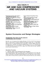
A construction-industry hoisting engine is to be designed to lower a maximum load
of 6000 lb (2724 kg) using a band brake, Fig. 1, having a 48-in (121.9-cm) drum
diameter and a drum width of 8-in (20.3-cm). The brake band width is 6-in (15.2-
cm) with an arc of contact of 300
Њ. Maximum distance for lowering a load is 200
ft (61 m). The cycle of the engine is 1.5 min hoisting and 0.75 min lowering, with
0.3 min for loading and unloading. If a temperature rise of 300
ЊF (166.5ЊC) is
permitted, determine the heat generated, radiating surface required, and the actual
temperature rise of the drum if the brake is made of cast iron and weighs 600 lb
(272.4 kg).
Calculation Procedure:
1. Determine the heat generated, equivalent to the power developed
Use the relation, H
g
ϭ (wd / T
L
)(33,000), where H
g
ϭ heat generated during low-
ering of the load of w, lb (kg), hp (kW); d
ϭ distance the load is lowered, ft (m);

T
L
ϭ time for lowering, minutes. Substituting for this hoisting engine, we have,
H
g
ϭ (6000)(200)/(0.75)(33,000) ϭ 48.48 hp (36.2 kW).
2. Find the load factor for the brake
The load factor, q, for a brake
ϭ T
L
/(T
H
ϩ T
L
ϩ T
LU
), where T
H
ϭ hoisting time,
minutes; T
LU
ϭ time to load and unload, minutes; other symbols as before. Sub-
stituting, q
ϭ (0.75)/(1.5 ϩ 0.75 ϩ 0.3) ϭ 0.294.
3. Compute the required radiating area for the brake
Use the relation, A
R
ϭ 42.4(q)(H
g
)/Ct

r
), where A
R
ϭ required radiating area, in
2
(cm
2
); Ct
r
ϭ brake radiating factor from Table 4. Assuming a temperature rise of
300
ЊF (166.7ЊC), and substituting, A
R
ϭ (42.4)(0.294)(48.5) / 0.25 ϭ 2418.3 in
2
(15,601.9 cm
2
).
It is necessary to assume a temperature rise when analyzing a brake because the
rise is a factor in the computation. Without such an assumption the required radi-
ating area cannot be determined.
Using the given dimensions for this brake, we can find the area of the drum
from A
d
ϭ 2(
␲
)(48 ϫ 8) Ϫ (
␲
)(48 ϫ 6)(300Њ/360Њ) ϭ 1657.9 in
2

(10,696.1 cm
2
).
Since the required radiating area is 2418 in
2
., as computed above, the excess area
required will be 2418
Ϫ 1658 ϭ 760 in
2
(4903.2 cm
2
). This area can be provided
Downloaded from Digital Engineering Library @ McGraw-Hill (www.digitalengineeringlibrary.com)
Copyright © 2006 The McGraw-Hill Companies. All rights reserved.
Any use is subject to the Terms of Use as given at the website.
MECHANICAL AND ELECTRICAL BRAKES
MECHANICAL AND ELECTRICAL BRAKES 24.7
FIGURE 1 (a) Self-locking band brake. (b) Pressure var-
iation along the surface of a band brake.
by the brake flanges and web. To be certain that sufficient area is available for heat
radiation, check the physical dimensions of the brake flanges and webs to see if
the needed surface is present.
4. Find the temperature rise during brake operation
The actual temperature of the brake drum will vary slightly above and below the
assumed 300
ЊF (166.7ЊC) temperature rise during operation. The reason for this is
because heat is radiated during the whole cycle of operation but is generated only
during the lowering cycle, which is 29.4 percent of the total cycle.
The temperature change of the drum during the braking operation will be T
r

ϭ
[1/(778)(W
r
)(c)][Wh Ϫ Ct
r
A
r
m(778)], where c ϭ specific heat of the drum
material
ϭ 0.13 for cast iron; m ϭ lowering time in minutes; other symbols
as given earlier. Substituting, T
r
ϭ [1/(778)(600)(0.13)][(6000 ϫ 200) Ϫ
(0.25)(2418)(0.75)(778)] ϭ 14ЊF (7.78ЊC). Thus, the drum temperature can range
Downloaded from Digital Engineering Library @ McGraw-Hill (www.digitalengineeringlibrary.com)
Copyright © 2006 The McGraw-Hill Companies. All rights reserved.
Any use is subject to the Terms of Use as given at the website.
MECHANICAL AND ELECTRICAL BRAKES
24.8 DESIGN ENGINEERING
about 14Њ, or about 7Њ above and 7Њ below the average operating temperature of
300
ЊF (148.9ЊC).
Related Calculations. The actual temperature attained by a brake drum, and
the time required for it to cool, cannot be accurately calculated. But the method
given here is suitable for preliminary calculations. In the final design of a new
brake, heating should be checked by a proportional comparison with a brake already
known to give good performance in actual service.
An approximation of the time required for a brake to cool can be made using
the relation given in step 2 of the previous procedure. Note that the value of K
selected in that relation will directly influence brake cooling time. Thus, a lower

value chosen for K will increase the estimated cooling time while a higher value
will decrease the time. For safety reasons, engineers will often select lower K values
so the brake will be given more time to cool, or will be provided with a larger
capacity cooling mechanism.
This procedure is the work of Alex Vallance, Chief Designer, Reed Roller Bit
Co. and Venton L. Doughtie, Professor of Mechanical Engineering, University of
Texas.
DESIGNING A BRAKE AND ITS ASSOCIATED
MECHANISMS
Design a hoist for the building industry to lift a cubic yard (0.76 m
3
) of concrete
at the rate of 200 ft/min (61 m / min). A cubic yard of concrete weighs approxi-
mately 400 lb (1816 kg) and the bucket weighs 1250 lb (568 kg). Since the hoist
may be used for other construction purposes, the design capacity will be 6000 lb
(2725 kg). There will be no counterweights in this hoist and the cable drum will
be connected to a 1750-r/min electric motor through a reduction gear train. Low-
ering will be controlled by manual operation of a brake. This brake must automat-
ically hold the load at any position when the motor is not driving the hoist. Figure
2 shows the proposed arrangement of parts and the limiting dimensions of this hoist
control. It has been proposed that a spring-loaded band brake be used that will be
manually released by the operator during lowering of the load. An overrunning
clutch is to be provided to disengage the brake automatically when the torque from
the motor through the gear train is sufficient to raise the load. Determine (a) the
dimensions q and n, Fig. 2, for maximum self-energization without self-locking if
the coefficient of friction,
␮
, varies between 0.20 and 0.50—the wide range is
selected to cover possible changes in service due to unavoidable entrance of small
amounts of water, oil, or dirt into the brake; (b) the spring force required to ensure

that the brake will not slip when
␮
is between 0.20 and 0.50; (c) the force exerted
by the operator when the rated load first starts to lower under normal conditions;
i.e., when
␮
ϭ 0.35; (d) the minimum width of brake lining; and (e) the maximum
lowering speed for a reasonable wear life.
Calculation Procedure:
1. Determine the actuating arm dimensions
The force F
1
and F
2
must act as shown, Fig. 2, for the braking torque to oppose
the load torque. This brake will be self-energizing when the F
1
moment tends to
Downloaded from Digital Engineering Library @ McGraw-Hill (www.digitalengineeringlibrary.com)
Copyright © 2006 The McGraw-Hill Companies. All rights reserved.
Any use is subject to the Terms of Use as given at the website.
MECHANICAL AND ELECTRICAL BRAKES
MECHANICAL AND ELECTRICAL BRAKES 24.9
SI Values
12 in. 30.5 cm
48 in. 121.9 cm
24 in. 60.9 cm
6000 lb 2724 kg
FIGURE 2 Band brake used in hoisting application.
apply the brake, that is q is less than n, and becomes self-locking when F

1
q Ն F
2
n.
The appropriate equation is
F
1
␮␪
ϭ e
F
2
and the critical design condition will be when F
1
/F
2
is a maximum,
␮
ϭ 0.50.
Thus,
Fn
1
␮␪
0.50
ϫ
(3 / 2)
␲
ϭϭe ϭ e ϭ 10.55
Fq
2
This unit will be most compact when q is as small as possible. The strengths of

the pin and the lever will be the major factors in determining the minimum dimen-
sion for q. However, if q is estimated to be 1.5 in (3.8 cm), it can be seen that
there is not enough space in which to place the lever, as shown, when n
ϭ 10.55q.
Therefore, under the specified conditions, it is not practical to use self-energization,
Downloaded from Digital Engineering Library @ McGraw-Hill (www.digitalengineeringlibrary.com)
Copyright © 2006 The McGraw-Hill Companies. All rights reserved.
Any use is subject to the Terms of Use as given at the website.
MECHANICAL AND ELECTRICAL BRAKES
24.10 DESIGN ENGINEERING
SI Values
48 in. 121.9 cm
12 in. 30.5 cm
2 in. 5.1 cm
FIGURE 3 Lever for band
brake actuation.
and the proposed design will be modified to make q ϭ 0, as shown in Fig. 3.
Choose the dimension n as 2.0 in (5.08 cm).
2. Find the required spring force
Maximum spring force will be required when the coefficient of friction is a mini-
mum, that is when
␮
ϭ 0.20. For this case,
F
1
␮␪
0.20
ϫ
(3 / 2)
␲

ϭ e ϭ e ϭ 2.57
F
2
and
F
ϭ 2.57F
12
D
T ϭ (F Ϫ F )
12
2
and
Downloaded from Digital Engineering Library @ McGraw-Hill (www.digitalengineeringlibrary.com)
Copyright © 2006 The McGraw-Hill Companies. All rights reserved.
Any use is subject to the Terms of Use as given at the website.
MECHANICAL AND ELECTRICAL BRAKES
MECHANICAL AND ELECTRICAL BRAKES 24.11
D
cable drum
T ϭ F ϭ 6000 ϫ 24/2 ϭ 72,000 lb ⅐ in. (8136 N ⅐ m)
cable
2
D
ϭ 30/2 ϭ 15 in (38.1 cm)
2
Solving for F
1
, we find
F
ϭ F ϩ 4800 lb

12
Solving the two equations above simultaneously, we find
F
ϭ 3060 lb (13,611 N)
2
and
F
ϭ 7860 lb (34,961 N)
1
͚M ϭ 0
O
F ϫ 12 Ϫ F ϫ 2 ϭ F ϫ 12 Ϫ 3060 ϫ 2 ϭ 0
s 2 s
Solving for the spring force we find it to be 510 lb (2268 N).
3. Compute the operating force for rated load under normal conditions
The operator must push the lever to the right to lower the load. When
␮
ϭ 0.35,
F
1
␮␪
0.35
ϫ
(3 / 2)
␲
ϭ e ϭ e ϭ 5.20
F
2
and
F

ϭ 5.20F
12
Solving the equations for force simultaneously, we find
F
ϭ 5940 lb (26421 N) F ϭ 1140 lb (5071 N)
12
Then,
͚M ϭ 0
O
ϪP ϫ 48 ϩ F ϫ 12 Ϫ F ϫ 2 ϭ 0
s 2
ϪP ϫ 48 ϩ 510 ϫ 12 Ϫ 1140 ϫ 2 ϭ 0
Solving for P,wefindP
ϭ 80 lb (356 N). This force is too large for an operator
to exert and the situation becomes even worse when the hoist is lightly loaded.
For example, if the load is considered to be negligible, the force required to
release the brake will be 510/4
ϭ 127.5 lb (567 N). A reasonable design solution
would be to use a compound lever, Fig. 4, in place of the single lever we have
been analyzing. A force of 30 lb (133 N) will be satisfactory for releasing the brake
when the load is negligible.
Based on the analysis above, we shall consider 2 in (5.08 cm) as the value for
the distance from the point of spring attachment to the pin B on lever 2, Fig. 4. It
Downloaded from Digital Engineering Library @ McGraw-Hill (www.digitalengineeringlibrary.com)
Copyright © 2006 The McGraw-Hill Companies. All rights reserved.
Any use is subject to the Terms of Use as given at the website.
MECHANICAL AND ELECTRICAL BRAKES
24.12 DESIGN ENGINEERING
SI Values
48 in. 121.9 cm

34 in. 86.4 cm
2 in. 5.1 cm
12 in. 30.5 cm
FIGURE 4 Compound lever for band
brake.
should be noted that the operator must now pull the lever to the left to release the
brake. Taking moments we have:
͚M ϭ 0
O
2
ϪF ϫ 14 ϩ F ϫ 12 ϭϪF ϫ 14 ϩ 510 ϫ 12 ϭ 0
Bs B
F ϭ 437 lbfrom which
B
͚M ϭ 0
O
3
Pb Ϫ Faϭ 30 ϫ (34 Ϫ a) Ϫ 437a ϭ 0
B
a ϭ 2.18 infrom which
b
ϭ 34 Ϫ 2.18 ϭ 31.82 inand
Downloaded from Digital Engineering Library @ McGraw-Hill (www.digitalengineeringlibrary.com)
Copyright © 2006 The McGraw-Hill Companies. All rights reserved.
Any use is subject to the Terms of Use as given at the website.
MECHANICAL AND ELECTRICAL BRAKES
MECHANICAL AND ELECTRICAL BRAKES 24.13
TABLE 5 Coefficients of Friction and Allowable Pressures
Material
␮

p, lb/in
2
kPa
Asbestos in rubber compound, on metal
Asbestos in resin binder, on metal:
Dry
In oil
Sintered metal on cast iron:
Dry
In oil
0.3–0.4
0.3–0.4
0.10
0.20–0.40
0.05–0.08
75–100
75–100
600
400
516.8–689.0
516.8–689.0
4134.0
2756.0
pV Ϲ 30,000 for continuous application of load and poor dissipation of heat.
pV
Ϲ 60,000 for intermittent application of load, comparatively long periods of rest, and poor dissipation
of heat.
pV
Ϲ 84,000 for continuous application of load and good dissipation of heat, as in an oil bath.
The operating force for rated load with the compound lever under normal con-

ditions is:
͚M ϭ 0
O
2
ϪF ϫ 14 ϩ F ϫ 12 Ϫ F ϫ 2 ϭϪF ϫ 14 ϩ 510 ϫ 12 Ϫ 1,140 ϫ 2 ϭ 0
Bs2 B
F ϭ 274 lb
B
͚M ϭ 0
O
3
P ϫ 31.82 Ϫ F ϫ 2.18 ϭ P ϫ 31.82 Ϫ 274 ϫ 2.18 ϭ 0
B
from which
Solving for P, we find it to be 18.8 lb (83.6 N), which is satisfactory.
4. Determine the required width of the brake lining
Design data specifically applicable to band brakes are not available. Hence, we
must use the information available for shoe brakes given in Table 5. The main
difficulty is that the pressure distribution for band brakes is much less uniform than
for shoe brakes. Hence, data based on projected area must be used with caution. A
conservative procedure will be to calculate the band width by limiting the maximum
value of the pressure, p, and the product of the pressure and the velocity, pV,to
those given for shoe brakes, based on the projected area of the brake. The maximum
pressure will be limited to 100 lb/in
2
(689 kPa).
The basic relation for band width, b,is
FF
b ϭϭ
pR pD/2

When the hoist is used to raise concrete, the lowering load will be essentially
the weight of the bucket and adhering concrete. But, since the hoist will be sold
for general use, the brake should have a reasonable wear life with the rated load
of 6000 lb (2724 kg) under normal conditions, i.e., with
␮
ϭ 0.35. The maximum
pressure will be at the F
1
end of the lining, Fig. 2. Since F
1
was determined for
these conditions, in the calculations for operating force, to be 5940 lb (26,421 N),
Downloaded from Digital Engineering Library @ McGraw-Hill (www.digitalengineeringlibrary.com)
Copyright © 2006 The McGraw-Hill Companies. All rights reserved.
Any use is subject to the Terms of Use as given at the website.
MECHANICAL AND ELECTRICAL BRAKES
24.14 DESIGN ENGINEERING
5940
b ϭϭ3.96 or 4 in (10.2 cm)
30
100 ϫ ⁄2
5. Compute lowering velocity of the brake
The brake will be in almost continuous use for relatively long periods of time;
therefore, pV will be limited to 30,000. Thus
pV
30,000
V ϭϭ ϭ300 ft / min (91.4 m / min)
p 100
The load velocity corresponding to the brake sliding velocity of 300 ft/min (91.4
m/min) will be

24
V ϭ 300 ϫ ⁄30 ϭ 240 ft/min (73.2 m / min)
load
Summarizing this design we have the following: Brake lever—compound lever,
tight side of band to pivot—see Fig. 4; Spring force
ϭ 510 lb (2268 N); release
force
ϭ 18.8 lb (80.1 N) with rated load of 6000 lb (2724 kg) and
␮
ϭ 0.35; lining
width
ϭ 4 in (10.2 cm); lowering velocity ϭ 240 ft / min (91.4 m/min) with rated
load of 6000 lb (2724 kg).
Related Calculations. The primary function of a brake is to slow, and stop,
the rotation of a shaft. No matter where a brake is used, it will have the stopping
of the rotation of a shaft as its primary function.
Thus, brakes used in hoists, such as this one, elevators, motor vehicles, aircraft
landing gears, etc., all stop, or slow, a rotating shaft. Energy absorbed by the brake
during its stopping or slowing action is dissipated as heat. In some applications,
such as motor vehicles and aircraft, the brake is usually outdoors where there is an
infinite heat sink to absorb the dissipated heat. But in other applications, such as
passenger elevators, the brake may be indoors where heat dissipation is not as
certain because the heat sink may be restricted by enclosures, heating systems, etc.
Hence, careful analysis of the brake operating temperature is necessary.
Three factors governing brake performance are (1) the pressure between the
brake shoe and drum; (2) the coefficient of friction of the brake-shoe lining material;
(3) the heat dissipating capacity of the brake. Each of these must be checked care-
fully before accepting a final brake design.
Brakes may also be used to position a part at rest or prevent an unwanted reversal
of the direction of rotation of a shaft. With the greater attention to environmental

aspects of machine design today, asbestos brake linings are receiving intense study
because of the nature of this material. Asbestos is used in several brakes types
—shoe, band, and disk—it is not used in hydrodynamic brakes. The major dis-
advantage of the hydrodynamic brake is that it cannot stop motion entirely and a
shoe or band brake is required to stop the motion and hold the member in position.
A hydrodynamic brake is essentially a fluid coupling with the output rotor stationary
so the coupling operates with 100 percent slip at all times. Water is generally used
as the fluid.
Disk brakes are becoming more popular every year. They are used on automo-
biles, airplanes, bicycles, trains, and trucks. Almost all the newer designs have the
anti-locking feature which prevents accidents from locked brakes. Advantages cited
for disk brakes are increased braking surface and better heat dissipation.
This procedure is the work of Richard M. Phelan, Associate Professor of Me-
chanical Engineering, Cornell University.
Downloaded from Digital Engineering Library @ McGraw-Hill (www.digitalengineeringlibrary.com)
Copyright © 2006 The McGraw-Hill Companies. All rights reserved.
Any use is subject to the Terms of Use as given at the website.
MECHANICAL AND ELECTRICAL BRAKES
MECHANICAL AND ELECTRICAL BRAKES 24.15
(a)(b)
(c)
FIGURE 5 (a) Internal shoe brake with single actuating cylinder. (b) Dual actuating cylinders.
(c) Mathematical relations for an internal shoe brake.
INTERNAL SHOE BRAKE FORCES AND TORQUE
CAPACITY
An internal shoe brake of the type shown in Fig. 5 has a diameter of 12 in (30.5
cm). The actuating forces F are equal and the shoes have a face width of 1.5 in
Downloaded from Digital Engineering Library @ McGraw-Hill (www.digitalengineeringlibrary.com)
Copyright © 2006 The McGraw-Hill Companies. All rights reserved.
Any use is subject to the Terms of Use as given at the website.

MECHANICAL AND ELECTRICAL BRAKES
24.16 DESIGN ENGINEERING
(3.8 cm). For a coefficient of friction of 0.3 and a maximum permissible pressure
of 150 lb/in
2
(1033.5 kPa), with
␪
1
ϭ 0,
␪
2
ϭ 130Њ,
␪
m
ϭ 90Њ, a ϭ 5 in (12.7 cm),
and c
ϭ 9 in (22.9 cm), determine the value of the actuating forces F and the brake
torque capacity.
Calculation Procedure:
1. Find the moment of the frictional forces about the brake-shoe pivot
The moment of the frictional forces, M
ƒ
, about the right-hand pivot of the brake is
given by
␪
2
ƒpwr ƒpwr
1
mm
2

M ϭ ͵ (sin
␪
)(r Ϫ a cos
␪
) d
␪
ϭ r Ϫ r cos
␪
Ϫ a sin
␪
ͫͬ
ƒ 22
0
sin
␪
sin
␪
2
mm
2
ϭ 3400 in ⅐ lb (384.2 N ⅐ m)(0.03)(150)(1.5)(6)[6 ϩ 6(0.643) Ϫ 2.5(0.766) ]
where ƒ
ϭ coefficient of friction; p
m
ϭ maximum permissible pressure on the shoe,
lb/in
2
(kPa); w ϭ band width, in (cm); r ϭ brake radius, in (cm); other symbols as
given in Fig. 5c.
2. Compute the moment of the normal forces about the brake-shoe pivot

The moment, M
n
, of the normal forces about the right-hand pivot is given by
␪
2
pwra pwra
11
mm
2
M ϭ ͵ sin
␪
d
␪
ϭ
␪
Ϫ sin 2
␪
ͫͬ
n 22
0
sin
␪
sin
␪
24
mm
ϭ 9300 in ⅐ lb (1050.9 N ⅐ m)
F
ϭ (M Ϫ M )/c ϭ (9300 Ϫ 3400)/9 ϭ 656 lb (2917.9 N)
n ƒ

where the symbols are as given earlier and in the procedure statement.
3. Determine the brake torque capacity
The brake torque capacity of the right shoe is
cos
␪
Ϫ cos
␪
12
2
T ϭ ƒpwr ϭ 4000 lb (17,792 N)
ͩͪ
m
sin
␪
m
For the left shoe, T ϭ 1860 in ⅐ lb (210.2 N ⅐ m) based on ϭ 69.7 lb / in
2
pЈ
m
(480.2 kPa) from
Fcp
m
pЈ ϭ
m
M ϩ M
n ƒ
4. Find the brake torque capacity
The total torque, or brake torque, capacity
ϭ 4000 ϩ 180 ϭ 5860 in ⅐ lb (662.2
N

⅐ m).
Related Calculations. Internal brake shoes are popular in a variety of appli-
cations including vehicles of various types, hoisting machinery, etc. Figures 5a and
5b show vehicle application with hydraulic cylinders for actuation of the internal
shoes. Disk brakes are more popular today in automobile applications because they
have a number of advantages over internal shoe brakes.
Downloaded from Digital Engineering Library @ McGraw-Hill (www.digitalengineeringlibrary.com)
Copyright © 2006 The McGraw-Hill Companies. All rights reserved.
Any use is subject to the Terms of Use as given at the website.
MECHANICAL AND ELECTRICAL BRAKES
MECHANICAL AND ELECTRICAL BRAKES 24.17
This procedure is the work of Allen S. Hall, Jr., Professor of Mechanical En-
gineering, Purdue University; Alfred R. Holowenko, Professor of Mechanical
Engineering, Purdue University; and Herman G. Laughlin, Associate Professor of
Mechanical Engineering, Purdue University.
ANALYZING FAILSAFE BRAKES FOR MACHINERY
Determine the torque that a brake must handle when the power to be dissipated by
the brake is 5 hp (3.7 kW) at 3600 r/min. The duty cycle (number of times the
brake is used) is frequent. Show how to compute the brake torque, energy absorbed
per stop, heat produced by the brake, temperature rise from brake-generated heat,
average brake-disk temperature, peak temperature of the brake, and the service life
of the brake.
Calculation Procedure:
1. Find the torque the brake must handle
The torque a brake must handle is given by T
ϭ 5250PK/s, where T ϭ torque
brake handles, lb
⅐ ft (N ⅐ m); P ϭ hp absorbed (kW); K ϭ a safety factor which
varies between 1.5 and 5 as the duty cycle of the brake increases; s
ϭ brake rotation

speed, rpm. Substituting for this brake using a value of K
ϭ 5 because this brake
is used frequently, T
ϭ 5250(5)(5)/3600 ϭ 36.46 lb ⅐ ft (49.4 N ⅐ m).
This equation may be the only means available for brake selection, especially
if the actual load torques are difficult to calculate and the inertia of the system
cannot be determined.
Torque can also be computed from T
ϭ WR
2
⌬s/308t, where W ϭ weight of
body stopped, lb (kg); R
ϭ radius of gyration, ft (m); ⌬s ϭ change in speed of the
brake, rpm. Note that this expression takes into account the torque necessary to
overcome the inertia of the system. However, it is important to note that frictional
torque is not considered in this relationship.
2. Show how to compute the energy absorbed per brake stop
In general, the major factor influencing brake service life is the energy absorbed
per stop and the resulting heat produced in the friction material. For a caliper brake,
the energy absorbed by the brake per stop is: E
s
ϭ WR
2
N
2
/5872, where E
s
ϭ energy
absorbed per stop, ft
⅐ lb (N ⅐ m); R ϭ radius of gyration, ft (m); N ϭ number of

turns to stop. This expression, as the second one in step 1, uses the inertia of the
system. Hence, the designer faces the necessity of either determining, by compu-
tation, the inertia of the system, or having it supplied by the machine builder.
3. Find the heat produced in the brake
The heat produced in the brake by the energy absorbed is found from H
ϭ E
s
/
778.3, where H
ϭ heat absorbed per stop, Btu (kJ).
4. Compute the temperature rise of the brake
The temperature rise resulting from the heat produced in the brake is T
r
ϭ
H/0.12W, where T
r
ϭ temperature rise per stop, ЊF(ЊC).
Downloaded from Digital Engineering Library @ McGraw-Hill (www.digitalengineeringlibrary.com)
Copyright © 2006 The McGraw-Hill Companies. All rights reserved.
Any use is subject to the Terms of Use as given at the website.
MECHANICAL AND ELECTRICAL BRAKES
24.18 DESIGN ENGINEERING
Open caliper disc
External drum and shoe
Internal drum and shoe
Enclosed multiple disc
Enclosed single disc
Brake Types
Torque Capability
Torque Capacity

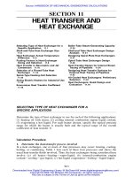
FIGURE 6 Comparison of the operating characteristics of five
different types of failsafe brakes. (Machine Design.)
5. Calculate the average disk temperature per stop
Use the relation T
d
ϭ HT
a
/2.25A, T
d
ϭ disk temperature per stop, ЊF(ЊC); T
a
ϭ
average disk temperature, ЊF(ЊC); A ϭ disk surface area, ft
2
(m
2
). In this expression
the factor 2.25 is the cooling index used when the disk is stationary during
cooling—the usual condition following an emergency stop. However, if the disk
rotates during cooling, a factor of 4.5 should be used instead.
6. Compute the peak temperature of the brake
The peak temperature of the brake is T
p
ϭ T
d
ϩ 0.5T
r
, where all the temperatures
are either in
ЊFor(ЊC).

7. Find the brake service life
To find the service life, L, in number of stops for a brake, use the relation, L
ϭ
(1.98 ϫ 10
6
)ZY/E
s
, where the service factor, Z, is found from standard curves
available from brake manufacturers and friction-material suppliers; Y
ϭ total friction
material volume, in
3
(cm
3
).
Related Calculations. Failsafe brakes are ‘‘opposite-mode’’ devices that acti-
vate when a machine is off and disengage when the machine is on. These brakes
store energy that is released to apply the brake when the machine’s power supply
is either turned off intentionally or lost through an equipment malfunction. In this
manner failsafe brakes provide a reliable method for automatically stopping a po-
tentially dangerous machine. Figure 6 compares brake characteristics for five dif-
ferent types of failsafe brakes.
Downloaded from Digital Engineering Library @ McGraw-Hill (www.digitalengineeringlibrary.com)
Copyright © 2006 The McGraw-Hill Companies. All rights reserved.
Any use is subject to the Terms of Use as given at the website.
MECHANICAL AND ELECTRICAL BRAKES
MECHANICAL AND ELECTRICAL BRAKES 24.19
Failsafe brake characteristics are difficult to compare quantitatively because they
depend on many operating variables such as load, weight, speed, and environment.
The dimensionless curves in Fig. 6 are useful, however, in positioning the various

failsafe brakes available. These curves indicate general trends for important oper-
ating characteristics, engagement, and disengagement methods.
High torque capability is generally associated with a proportionately low energy
capacity for each brake. These torque and energy limits are primarily due to the
rate at which the brake dissipates heat and the ability of the brake material to
withstand high temperatures.
The most common type of failsafe brake is the energy-absorbing or dynamic
brake that decelerates a rotating shaft or other machine part until it comes safely
to rest. A second type, called a parking or static brake, holds the position of a
moving part after it has been stopped. Both types apply braking force in the absence
of normal equipment power.
Failsafe brakes are used in almost any type of equipment that contains moving
parts. Applications include shears, punch presses, machine tools, and other manu-
facturing equipment. Public conveyances using these brakes include trains and el-
evators. Large pieces of farm and construction machinery use failsafe brakes along
with missile launchers, antenna drives, and other aerospace equipment.
The brakes used in these heavy-duty applications typically are large devices
capable of dissipating high levels of kinetic energy to stop machines quickly. How-
ever, not all failsafe brakes are used on large equipment. Because of OSHA restric-
tions, failsafe brakes are being used increasingly on consumer-operated power
equipment such as garden tractors, lawn mowers, and golf carts. Failsafe brakes are
also being used on the mechanical portions of electronic equipment, such as com-
puters and medical equipment.
In any failsafe brake, the release element that overcomes the force of brake
engagement may consist of a hydraulic, pneumatic, or electrical system. Friction
surfaces are molded phenolics, copper, brass, ceramics in a sintered matrix, sintered
iron, or sintered brass. Maple blocks have also been used.
Electric, hydraulic, and pneumatic release systems have high torque capability
and response speed. Pneumatic release systems are often used because they are
relatively inexpensive, safe, clean, and simple to install and maintain. Mechanical

release systems provide the lowest torque and speed capabilities and are used only
in a few limited applications.
The equations and data in this procedure are the work of Herbert S. Peterson,
President, Simplatrol Products; Jack W. Moss, Chief Engineer, Wichita Clutch; and
Roger W. Eisbrener, Marketing Manager, Formsprag-Gerbing, as reported in Ma-
chine Design magazine. SI values were added by the handbook editor.
Downloaded from Digital Engineering Library @ McGraw-Hill (www.digitalengineeringlibrary.com)
Copyright © 2006 The McGraw-Hill Companies. All rights reserved.
Any use is subject to the Terms of Use as given at the website.
MECHANICAL AND ELECTRICAL BRAKES
Downloaded from Digital Engineering Library @ McGraw-Hill (www.digitalengineeringlibrary.com)
Copyright © 2006 The McGraw-Hill Companies. All rights reserved.
Any use is subject to the Terms of Use as given at the website.
MECHANICAL AND ELECTRICAL BRAKES