Encyclopedic Dictionary of International Finance and Banking Phần 8 docx

228 POLITICAL RISK

EXHIBIT 89
Euromoney Magazine’
s Country Risk Ratings, September 2000 (continued)


Total
Score
Political
Risk
Economic
Performance
Debt
Indicators
Debt in
Default or
Rescheduled
Credit
Ratings
Sep-00 Mar-00
Weighting: 100 25
25
10
10
10

79 85 Bolivia
42.52 8.54 7.10
8.08 10.00 2.81

80 84 Bulgaria
42.51 10.46 6.69
8.23 10.00 1.88
81 88 Kazakhstan
42.46 9.28 6.65
9.21 10.00 2.29
82 86 Paraguay
41.31 9.74 7.01
9.45 10.00 1.88
83 80 Iran
40.64 8.99 7.09
9.25 10.00 1.25
84 82 Belize
40.61 10.81 5.30
8.82 10.00 3.13
85 79 Sri Lanka

39.81 9.37 5.82
9.08 10.00 0.00
86 91 Seychelles
39.71 9.14 6.32
9.14 10.00 0.00
87 94 Macau
39.59 14.15 12.75
0.00
0.00 5.63
88 125 Maldives
39.22 9.64 8.23
9.03 10.00 0.00
89 92 Peru

39.12 10.63 7.50
9.15
1.25 3.33
90 93 Syria
38.95 9.67 6.62
7.96 10.00 0.00
91 116 Honduras
38.77 8.00 7.12
8.13 10.00 1.25
92 136 Dominica
38.60 7.39 9.98
9.08 10.00 0.00
93 115 Indonesia
38.48 7.98 5.96
6.65
8.65 0.63
94 87 Vietnam
38.36 9.82 6.01
8.64
9.96 1.88
95 133 Russia
37.88 8.02 6.65
8.62
8.26 0.42
96 99 Algeria
37.71 8.27 6.77
7.94
8.90 0.00
97 72 Ghana
37.64 8.57 6.61

7.92 10.00 0.00
98 89 Kenya
37.64 7.41 7.37
8.61 10.00 0.00
99 102 Gambia
37.63 7.85 7.67
9.43 10.00 0.00
100 120 Macedonia (FYR)

37.37 6.30 7.67
8.18 10.00 0.00
101 83 Papua New Guinea

37.17 8.49 5.33
8.74 10.00 2.29
102 103 Azerbaijan
36.94 8.42 6.72
9.22 10.00 0.00

SL2910_frame_CP.fm Page 228 Thursday, May 17, 2001 9:10 AM

POLITICAL RISK 229

103 107 Romania
36.62 8.17 5.32
8.89 10.00
0.83
104 100 Lesotho
36.42 8.47 6.74
8.54 10.00

0.00
105 98 St Lucia

35.91 9.98 4.57
8.69 10.00
0.00
106 118 Kyrgyz Republic

35.76 8.05 8.13
8.59 10.00
0.00
107 110 Equatorial Guinea

35.69 4.19 9.88
8.93 10.00
0.00
108 95 Bangladesh
34.96 7.73 5.48
9.24 10.00
0.00
109 96 Senegal
34.28 6.28 7.03
8.22 10.00
0.00
110 164 Uzbekistan
34.15 6.76 6.35
9.43 10.00
0.00
111 137 Yemen
33.99 7.57 5.86

8.38 9.95
0.00
112 101 Uganda
33.73 6.77 6.68
8.95 7.72
0.00
113 112 Zimbabwe
33.43 4.22 5.04
7.88 10.00
0.00
114 105 Cape Verde

33.06 6.33 4.95
8.89 10.00
0.00
115 134 Ukraine
33.06 6.05 5.68
9.26 9.61
0.00
116 97 Gabon
33.03 6.86 8.42
8.42 8.26
0.00
117 81 Swaziland
32.92 9.09 8.96
0.00 10.00
0.00
118 131 Cambodia
32.90 3.81 9.40
8.80 10.00

0.00
119 106 Nepal
32.72 6.24 5.38
8.96 10.00
0.00
120 123 Côte d’Ivoire
32.47 5.84 6.56
7.29 8.70
0.00
121 114 St Vincent & the Grenadines

32.14 7.53 4.27
7.70 10.00
0.00
122 108 Nigeria
32.09 4.88 6.20
8.48 10.00
0.00
123 129 Pakistan
31.99 6.36 4.87
8.61 10.00
0.94
124 119 Burkina Faso

31.95 6.27 4.65
8.85 10.00
0.00
125 132 Turkmenistan
31.81 5.98 5.96
7.32 10.00

0.94
126 109 Malawi
31.66 4.99 5.55
7.73 10.00
0.00
127 147 Samoa
31.28 7.75 0.87
8.52 10.00
0.00
128 130 Ethiopia
30.95 4.79 7.62
7.41 9.80
0.00
129 140 Belarus
30.74 5.77 3.24
9.82 10.00
0.00
130 139 Mongolia
30.64 6.10 3.68
8.71 10.00
1.25
131 144 Armenia
30.47 6.22 3.44
8.91 10.00
0.00
132 121 Grenada
30.41 8.09 1.46
8.71 10.00
0.00
133 155 Georgia

30.40 4.19 6.05
9.26 10.00
0.00
134 135 Solomon Islands

30.39 6.86 0.79
9.25 10.00
0.00
(

Continued

)

SL2910_frame_CP.fm Page 229 Thursday, May 17, 2001 9:10 AM

230 POLITICAL RISK

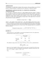
EXHIBIT 89
Euromoney Magazine’
s Country Risk Ratings, September 2000 (continued)


Total
Score
Political
Risk
Economic
Performance
Debt

Indicators
Debt in
Default or
Rescheduled
Credit
Ratings
Sep-00 Mar-00
Weighting: 100 25
25
10
10
10

135 146 Albania
30.38 5.40 4.56 9.49
10.00 0.00
136 127 Vanuatu
30.02 6.19 0.92 9.58
10.00 0.00
137 126 Cameroon
29.74 5.64 5.52
7.73
7.72 0.00
138 117 Madagascar
29.48 3.90 5.66
7.87
9.37 0.00
139 153 Ecuador
29.28 3.90 5.34
7.94 10.00 0.00

140 142 Moldova
29.24 4.90 2.42
8.37 10.00 0.94
141 113 Tanzania
28.89 4.96 6.12
6.63
8.79 0.00
142 145 Mozambique
28.63 4.60 5.48
6.31
8.84 0.00
143 111 Togo
28.63 5.46 3.61
7.69
9.19 0.00
144 157 Bhutan
28.53 6.19 0.71
9.22 10.00 0.00
145 141 Benin
28.51 4.00 3.69
8.64 10.00 0.00
146 152 Guyana
28.27 6.69 3.79
6.10 10.00 0.00
147 104 Mali
28.15 4.66 3.52
8.02
9.99 0.00
148 150 Chad
27.79 3.04 3.51

8.73
9.82 0.00
149 149 Mauritania
27.19 3.52 5.33
5.66 10.00 0.00
150 138 Zambia
27.04 3.86 6.35
6.57
9.32 0.00
151 122 Guinea
26.77 5.02 3.19
8.04
9.62 0.00
152 171 Myanmar
26.35 5.03 3.24
7.19 10.00 0.00
153 158 Nicaragua
26.34 4.71 5.76
4.29
8.72 1.25
154 154 Sudan
25.45 2.41 3.33
8.82 10.00 0.00
155 124 Niger
25.43 2.67 3.17
8.26
9.89 0.00
156
—
Micronesia (Fed. States)

25.24 13.06 0.93 0.00 10.00
0.00
157 156 Central African Republic
25.13 2.86 4.27 8.11
9.00 0.00
158 168 Djibouti
24.63 3.30 0.91
9.17 10.00 0.00
159 148 Haiti
24.32 2.71 0.69
9.40 10.00 0.00

SL2910_frame_CP.fm Page 230 Thursday, May 17, 2001 9:10 AM

POLITICAL RISK 231

160 128 Tonga
24.01 8.64 1.06
0.00 10.00
0.00
161 163 Laos
23.99 6.06 0.00
7.04 10.00
0.00
162 143 Namibia
23.65 10.29 7.58
0.00 0.00
0.00
163 176 Suriname
23.11 7.36 3.22

0.00 10.00
1.25
164 162 Sierra Leone

23.06 2.62 2.96
6.62 9.97
0.00
165 161 Dem. Rep. of the Congo (Zaire)

22.87 2.35 2.61
7.01 10.00
0.00
166
—
Eritrea
22.18 1.33 0.64
9.31 10.00
0.00
167 159 Congo
22.03 3.66 3.44
5.75 9.19
0.00
168 151 Rwanda
21.13 1.52 0.77
9.55 8.40
0.00
169 167 Angola
20.97 3.30 3.29
4.44 8.42
0.00

170
—
Burundi
20.81 2.29 0.62
7.01 10.00
0.00
171 166 Guinea-Bissau
20.04 4.19 2.56
2.47 9.93
0.00
172 165 New Caledonia

19.96 12.86 3.67
0.00 0.00
0.00
173
—
Marshall Islands

19.44 12.19 1.00
0.00 0.00
0.00
174 174 Antigua & Barbuda

19.43 4.61 2.87
0.00 10.00
0.00
175 169 Libya
19.30 9.20 8.19
0.00 0.00

0.00
176 172 Tajikistan
17.76 3.09 4.42
8.99 0.00
0.00
177 160 Sao Tome & Principe

16.67 2.41 0.65
0.00 10.00
0.00
178
—
Bosnia-Herzegovina
15.82 3.38 3.25
8.16 0.00
0.00
179 173 Liberia
15.30 3.91 0.85
0.00 10.00
0.00
180 175 Yugoslavia (Fed. Republic)

14.81 1.99 1.73
0.00 10.00
0.00
181 170 Somalia
14.76 2.29 0.74
0.00 10.00
0.00
182 177 Cuba

10.67 3.80 5.81
0.00 0.00
0.00
183 178 Iraq
9.04 2.36 5.80
0.00 0.00
0.00
184 179 Korea North

4.72 2.98 0.85
0.00 0.00
0.00
185 180 Afghanistan
2.81 0.00 1.56
0.00 0.00
0.00

Source

:



www.euromoney.com.

SL2910_frame_CP.fm Page 231 Thursday, May 17, 2001 9:10 AM

232

A. Methods for Dealing with Political Risk

To the extent that forecasting political risks is a formidable task, what can an MNC do
to cope with them? There are several methods suggested.
•

Avoidance

—Try to avoid political risk by minimizing activities in or with
countries that are considered to be of high risk and by using a higher discount
rate for projects in riskier countries.
•

Adaptation

—Try to reduce such risk by adapting the activities (for example, by
using hedging techniques).
•

Diversification

—Diversity across national borders, so that problems in one country
do not risk the company.
•

Risk transfer

—Buy insurance policies for political risks. Most developed nations
offer insurance for political risk to their exporters. Examples include: in the U.S.,
the

Eximbank

offers policies to exporters that cover such political risks as war,
currency inconvertibility, and civil unrest. Furthermore, the

Overseas Private
Investment Corporation



(OPIC)

offers policies to U.S. foreign investors to cover
such risks as currency inconvertibility, civil or foreign war damages, or expropri-
ation. In the U.K., similar policies are offered by the

Export Credit Guarantee
Department



(ECGD)

; in Canada, by the

Export Development Council



(EDC)

; and
in Germany, by an agency called

Hermes

.

PORTFOLIO-BALANCE APPROACH

See ASSET MARKET MODEL.

PORTFOLIO DIVERSIFICATION

The rationale behind portfolio diversification is the reduction of risk. The main method of
reducing the risk of a portfolio is the combining of assets which are not perfectly positively
correlated in their returns.

EXAMPLE 99

Consider the following two-asset portfolio:
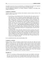
By changing the correlation coefficient, the benefits of risk reduction can be clearly observed,
as shown in Exhibits 90 and 91.

Stock Return Risk Correlation

Wal-mart (US) 18.60% 22.80% 0.20
Smith-Kline (UK) 16.00% 24.00%

EXHIBIT 90

Portfolio Analysis

Weight of
Wal-mart in
Portfolio
Weight of
Smith-Kline
in Portfolio
Expected
Return
(percent)
Expected Risk
(percent)

1.00 0.00 18.60% 22.80%
0.95 0.05 18.47% 21.93%
0.90 0.10 18.34% 21.13%
0.85 0.15 18.21% 20.41%
0.80 0.20 18.08% 19.77%
0.75 0.25 17.95% 19.22%
0.70 0.30 17.82% 18.78%

PORTFOLIO-BALANCE APPROACH

SL2910_frame_CP.fm Page 232 Thursday, May 17, 2001 9:10 AM

233

See also DIVERSIFICATION; EFFICIENT PORTFOLIO; INTERNATIONAL DIVERSIFI-
CATION; PORTFOLIO INVESTMENTS; PORTFOLIO THEORY.

PORTFOLIO INVESTMENTS

1. Investing in a variety of assets to reduce risk by diversification. An example of a portfolio
is a mutual fund that consists of a mix of assets which are professionally managed and
that seeks to reduce risk by diversification. Investors can own a variety of securities with
a minimal capital investment. Since mutual funds are professionally managed, they tend
to involve less risk. To reduce risk, securities in a portfolio should have negative or no
correlations to each other.

0.65 0.35 17.69% 18.44%
0.60 0.40 17.56% 18.22%
0.55 0.45 17.43% 18.11%
0.50 0.50 17.30% 18.13%
0.45 0.55 17.17% 18.27%
0.40 0.60 17.04% 18.52%
0.35 0.65 16.91% 18.89%
0.30 0.70 16.78% 19.36%
0.20 0.80 16.52% 20.60%
0.25 0.75 16.65% 19.94%
0.20 0.80 16.52% 20.60%
0.15 0.85 16.39% 21.35%
0.10 0.90 16.26% 22.17%
0.05 0.95 16.13% 23.06%
0.00 1.00 16.00% 24.00%

EXHBIT 91
Portfolio Analysis: Risk and Return Two Asset Portfolio

15.0
15.5
16.0
16.5
17.0
17.5
18.0
18.5
19.0
19.5
20.0
Return (%)
15.0 16.0 17.0 18.0 19.0 20.0 21.0 22.0 23.0 24.0 25.0
Risk (standard deviation, %)

PORTFOLIO INVESTMENTS

SL2910_frame_CP.fm Page 233 Thursday, May 17, 2001 9:10 AM

234

See also DIVERSIFICATION; EFFICIENT PORTFOLIO; INTERNATIONAL DIVERSIFI-
CATION; PORTFOLIO THEORY.
2. Investments that are undertaken for the sake of obtaining investment income or capital
gains rather than entrepreneurial income which is the case

with

foreign direct investments
(FDI )

. This typically involves the ownership of stocks and/or bonds issued by public or
private agencies of a foreign country. The investors are not interested in assuming control
of the firm.

PORTFOLIO THEORY

Theory advanced by H. Markowitz in attempting a well-diversified portfolio. The central
theme of the theory is that rational investors behave in a way that reflects their aversion to
taking increased risk without being compensated by an adequate increase in expected return.
Also, for any given expected return, most investors will prefer a lower risk, and for any given
level of risk, they will prefer a higher return to a lower return. Markowitz showed how
quadratic programming could be used to calculate a set of “efficient” portfolios. An investor
then will choose among a set of efficient portfolios the best that is consistent with the risk
profile of the investor.
Most financial assets are not held in isolation but rather as part of a portfolio. Therefore,
the risk–return analysis should not be confined to single assets only. What is important is the
expected return on the portfolio (not just the return on one asset) and the portfolio’s risk.
Most financial assets are not held in isolation; rather, they are held as parts of portfolios.
Therefore, risk–return analysis should not be confined to single assets only. It is important
to look at portfolios and the gains from diversification. What is important is the return on
the portfolio (not just the return on one asset) and the portfolio’s risk.

A. Portfolio Return

The expected return on a portfolio (

r

p

) is simply the weighted average return of the individual
sets in the portfolio, the weights being the fraction of the total funds invested in each asset:
where

r

j

= expected return on each individual asset

w

j

= fraction for each respective asset investment

n

= number of assets in the portfolio
= 1.0

EXAMPLE 100

A portfolio consists of assets A and B. Asset A makes up one-third of the portfolio and has an
expected return of 18%. Asset B makes up the other two-thirds of the portfolio and is expected
to earn 9%. The expected return on the portfolio is:

Asset Return (

r

j

) Fraction (

w

j

)

w

j

r

j

A 18% 1/3 1/3

×

18%

=

6%
B 9% 2/3 2/3

×

9%

=

6%

r

p



=

12%
r
p
w
1
r
1
w
2
r
2

…
w
n
r
n
+++ w
j
r
j
j =1
n
∑
==
w
j
j =1
n
∑
PORTFOLIO THEORY
SL2910_frame_CP.fm Page 234 Thursday, May 17, 2001 9:10 AM
235
B. Portfolio Risk
Unlike returns, the risk of a portfolio (
σ
p
) is not simply the weighted average of the standard
deviations of the individual assets in the contribution, for a portfolio’s risk is also dependent
on the correlation coefficients of its assets. The correlation coefficient (
ρ
) is a measure of the

degree to which two variables “move” together. It has a numerical value that ranges from
–1.0 to 1.0. In a two-asset (A and B) portfolio, the portfolio risk is defined as:
where
σ
A
and
σ
B
= standard deviations of assets A and B
w
A
and w
B
= weights, or fractions, of total funds invested in assets A and B
ρ
AB
= the correlation coefficient between assets A and B.
Incidentally, the correlation coefficient is the measurement of joint movement between two
securities.
C. Diversification
As can be seen in the above formula, the portfolio risk, measured in terms of
σ
is not the
weighted average of the individual asset risks in the portfolio. We have in the formula a third
term (
ρ
), which makes a significant contribution to the overall portfolio risk. What the formula
basically shows is that portfolio risk can be minimized or completely eliminated by diversi-
fication. The degree of reduction in portfolio risk depends upon the correlation between the
assets being combined. Generally speaking, by combining two perfectly negatively correlated

assets (
ρ
= −1.0), we are able to eliminate the risk completely. In the real world, however,
most securities are negatively, but not perfectly correlated. In fact, most assets are positively
correlated. We could still reduce the portfolio risk by combining even positively correlated
assets. An example of the latter might be ownership of two automobile stocks or two housing
stocks.
EXAMPLE 101
Assume the following:
The portfolio risk then is:
(a) Now assume that the correlation coefficient between A and B is +1 (a perfectly positive cor-
relation). This means that when the value of asset A increases in response to market conditions,
(Continued)
Asset
σσ
σσ
w
A 20% 1/3
B 10% 2/3
σ
p
w
A
2
σ
A
2
w
B
2

σ
B
2
2
ρ
AB
w
A
w
B
σ
A
σ
B
++=
σ
p
w
A
2
σ
A
2
w
B
2
σ
B
2
2

ρ
AB
w
A
w
B
σ
A
σ
B
++=
1/3()
2
0.2()
2
2/3()
2
0.1()
2
2
ρ
AB
1/3()2/3()0.2()0.1()++[]
1/2
=
0.0089 0.0089
ρ
AB
+=
PORTFOLIO THEORY

SL2910_frame_CP.fm Page 235 Thursday, May 17, 2001 9:10 AM
236
so does the value of asset B, and it does so at exactly the same rate as A. The portfolio risk when
ρ
AB
= +1 then becomes:
σ
p
= 0.0089 + 0.0089
ρ
AB
= 0.0089 + 0.0089(+1) = 0.1334 = 13.34%
(b) If
ρ
AB
= 0, the assets lack correlation and the portfolio risk is simply the risk of the expected
returns on the assets, i.e., the weighted average of the standard deviations of the individual assets
in the portfolio. Therefore, when
ρ
AB
= 0, the portfolio risk for this example is:
σ
p
= 0.0089 + 0.0089
ρ
AB
= 0.0089 + 0.0089(0) = 0.0089 = 8.9%
(c) If
ρ
AB

= −1 (a perfectly negative correlation coefficient), then as the price of A rises, the price
of B declines at the very same rate. In such a case, risk would be completely eliminated. There-
fore, when
ρ
AB
= −1, the portfolio risk is
σ
p
= 0.0089 + 0.0089
ρ
AB
= 0.0089 + 0.0089(−1) = 0.0089 − 0.0089 = 0 = 0
When we compare the results of (a), (b), and (c), we see that a positive correlation between
assets increases a portfolio’s risk above the level found at zero correlation, while a perfectly
negative correlation eliminates that risk.
EXAMPLE 102
To illustrate the point of diversification, assume data on the following three securities are as
follows:
Note here that securities X and Y have a perfectly negative correlation, and securities X and Z
have a perfectly positive correlation. Notice what happens to the portfolio risk when X and Y,
and X and Z are combined. Assume that funds are split equally between the two securities in
each portfolio.
Again, see that the two perfectly negative correlated securities (XY) result in a zero overall risk.
Year Security X (%) Security Y (%) Security Z (%)
20 × 1 10 50 10
20 × 2 20 40 20
20 × 3 30 30 30
20 × 4 40 20 40
20 × 5 50 10 50
r

j
30 30 30
σ
p
14.14 14.14 14.14
Year
Portfolio XY
(50% − 50%)
Portfolio XZ
(50% − 50%)
20 × 130 10
20 × 230 20
20 × 330 30
20 × 430 40
20 × 530 50
r
p
30 30
σ
p
0 14.14
PORTFOLIO THEORY
SL2910_frame_CP.fm Page 236 Thursday, May 17, 2001 9:10 AM
237
D. Markowitz’s Efficient Portfolio
Dr. Harry Markowitz, in the early 1950s, provided a theoretical framework for the systematic
composition of optimum portfolios. Using a technique called quadratic programming, he
attempted to select from among hundreds of individual securities, given certain basic infor-
mation supplied by portfolio managers and security analysts. He also weighted these selec-
tions in composing portfolios. The central theme of Markowitz’s work is that rational investors

behave in a way reflecting their aversion to taking increased risk without being compensated
by an adequate increase in expected return. Also, for any given expected return, most investors
will prefer a lower risk and, for any given level of risk, prefer a higher return to a lower
return. Markowitz showed how quadratic programming could be used to calculate a set of
“efficient” portfolios such as illustrated by the curve in Exhibit 92.
In Exhibit 93, an efficient set of portfolios that lie along the ABC line, called “efficient
frontier,” is noted. Along this frontier, the investor can receive a maximum return for a given
level of risk or a minimum risk for a given level of return. Specifically, comparing three
portfolios A, B, and D, portfolios A and B are clearly more efficient than D, because portfolio
A could produce the same expected return but at a lower risk level, while portfolio B would
have the same degree of risk as D but would afford a higher return.
To see how the investor tries to find the optimum portfolio, we first introduce the indifference
curve, which shows the investor’s trade-off between risk and return. Exhibit 94 shows the two
EXHIBIT 92
Efficient Frontier
Efficient Frontier
r
p
σ
p
PORTFOLIO THEORY
SL2910_frame_CP.fm Page 237 Thursday, May 17, 2001 9:10 AM
238
different indifference curves for two investors. The steeper the slope of the curve, the more
risk averse the investor is. For example, investor B’s curve has a steeper slope than investor
A’s. This means that investor B will want more incremental return for each additional unit
of risk.
EXHIBIT 93
Efficient Portfolio
EXHIBIT 94

Risk–Return Indifference Curves
A
B
C
D
Investor B
Investor A
PORTFOLIO THEORY
SL2910_frame_CP.fm Page 238 Thursday, May 17, 2001 9:10 AM
239
Exhibit 95 depicts a family of indifference curves for investor A. The objective is to
maximize his satisfaction by attaining the highest curve possible.
By matching the indifference curve showing the risk–return trade-off with the best invest-
ments available in the market as represented by points on the efficient frontier, investors are
able to find an optimum portfolio. According to Markowitz, investor A will achieve the highest
possible curve at point B along the efficient frontier. Point B is thus the optimum portfolio
for this investor.
E. Portfolio Selection as a Quadratic Programming Problem
A portfolio selection problem was formulated by Markowitz as a quadratic programming
model as follows:
Minimize E(r
p
) −
λ
V(r
p
)
subject to
Σx
i

= 1, (i = 1, 2, … n)
x
i
≥ 0
where
E(r
p
) = the expected return
V(r
p
) = the variance or covariance of any given portfolio
x
i
= proportion of the investor’s total investment in security i
EXHIBIT 95
Matching the Efficient Frontier and Indifference Curve
A
B
PORTFOLIO THEORY
SL2910_frame_CP.fm Page 239 Thursday, May 17, 2001 9:10 AM
240
n = number of securities
λ
(Lamda) = coefficient of risk aversion.
λ
represents the rate at which a particular investor is just willing to exchange expected
rate of return for risk.
λ
= 0 indicates the investor is a risk lover, while
λ

= 1 means he is a
risk averter. The resulting solution to the problem would identify a portfolio that lies on the
efficient portfolio. If one knows the coefficient of risk aversion,
λ
, for a particular investor,
the model will be able to find the optimal portfolio for that investor.
F. The Market Index Model
For even a moderately sized portfolio, the formulas for portfolio return and risk require
estimation of a large number of input data. Concern for the computational burden in deriving
these estimates led to the development of the following market index model:
r
j
= a + br
m
where
r
j
= return on security j
r
m
= return on the market portfolio
b = the beta or systematic risk of a security.
What this model attempts to do is measure the systematic or uncontrollable risk of a security.
The beta is measured as follows:
where
Cov(r
j
, r
m
) = the covariance of the returns of the security with the market return.

= the variance (standard deviation squared) of the market return, which is
the return on the Standard & Poor’s 500 or Dow Jones 30 Industrials.
An easier way to compute beta is to determine the slope of the least-squares linear
regression line (r
j
− r
f
), where the excess return of the security (r
j
− r
f
) is regressed against
the excess return of the market portfolio (r
m
− r
f
). The formula for beta is:
where M = (r
m
− r
f
), K = (r
j
− r
f
), n = the number of periods, = the average of M, and
= the average of K.
The market index model was initially proposed to reduce the number of inputs required
in portfolio analysis. It can also be justified in the context of the capital asset pricing model.
G. The Capital Asset Pricing Model (CAPM)

The capital asset pricing model (CAPM) takes off where the efficient frontier concluded with
an assumption that there exists a risk-free security with a single rate at which investors can
borrow and lend. By combining the risk-free asset and the efficient frontier, we create a whole
new set of investment opportunities which will allow us to reach higher indifference curves
than would be possible simply along the efficient frontier. The r
f
mx line in Exhibit 96 shows
this possibility. This line is called the capital market line (CML) and the formula for this line is:
r
p
= r
f
+ [(r
m
− r
f
)/(
σ
m
− 0)]
σ
p
b Cov r
j
, r
m
()/
σ
m
2

=
σ
m
2
b
MK
∑
nMK–


/
M
2
∑
nM
2
–


=
M
K
PORTFOLIO THEORY
SL2910_frame_CP.fm Page 240 Thursday, May 17, 2001 9:10 AM
241
which indicates the expected return on any portfolio (r
p
) is equal to the risk-free return (r
f
)

plus the slope of the line times a value along the horizontal axis (
σ
p
) indicating the amount
of risk undertaken.
H. The Security Market Line
We can establish the trade-off between risk and return for an individual security through the
security market line (SML) in Exhibit 97. SML is a general relationship to show the risk–return
trade-off for an individual security, whereas CML achieves the same objective for a portfolio.
The formula for SML is:
r
j
= r
f
+ b(r
m
− r
f
)
where
r
j
= the expected (or required ) return on security j
r
f
= the risk-free security (such as a T-bill)
r
m
= the expected return on the market portfolio (such as Standard & Poor’s 500 Stock
Composite Index or Dow Jones 30 Industrials)

b = beta, an index of nondiversifiable (noncontrollable, systematic) risk
This formula is called the Capital Asset Pricing Model (CAPM). The model shows that
investors in individual securities are only assumed to be rewarded for systematic, uncontrol-
lable, market-related risk, known as the beta (b) risk. All other risk is assumed to be diversified
away and thus is not rewarded.
The key component in the CAPM, beta (b), is a measure of the security’s volatility relative
to that of an average security. For example, b = 0.5 means the security is only half as volatile,
or risky, as the average security; b = 1.0 means the security is of average risk; and b = 2.0 means
the security is twice as risky as the average risk. The whole term b(r
m
− r
f
) represents the risk
premium, the additional return required to compensate investors for assuming a given level of risk.
Thus, in words, the CAPM (or SML) equation shows that the required (expected) rate of
return on a given security (r
j
) is equal to the return required for securities that have no risk
EXHIBIT 96
Graph of CAPM
m
x
r
f
PORTFOLIO THEORY
SL2910_frame_CP.fm Page 241 Thursday, May 17, 2001 9:10 AM
242
(r
f
) plus a risk premium required by investors for assuming a given level of risk. The higher

the degree of systematic risk (b), the higher the return on a given security demanded by
investors. Exhibit 97 shows the graph of the equation, known as the security market line
(SML).
EXAMPLE 103
Assuming that the risk-free rate (r
f
) is 8%, and the expected return for the market (r
m
) is 12%,
then if
See also BETA; DIVERSIFICATION; EFFICIENT PORTFOLIO; INTERNATIONAL
DIVERSIFICATION; PORTFOLIO INVESTMENTS.
POUND
Monetary unit of Great Britain, Cyprus, Egypt, Gibraltar, Republic of Ireland, Lebanon,
Malta, Sudan, and Syria.
PREMIUM
1. The price agreed upon between the purchaser and seller for the purchase or sale of an
option—purchasers pay the premium and sellers (writers) receive the premium.
2. The excess of one futures contract price over that of another, or over the cash market price.
PRIVATE EXPORT FUNDING CORPORATION
Private Export Funding Corporation (PEFCO) is a private U.S. corporation, established with
government support, which helps finance U.S. exports of big-ticket items from private sources.
PEFCO purchases at fixed interest rates the medium- to long-term debt obligations of importers
EXHIBIT 97
The Security Market Line (SML)
b = 0 (risk-free security) r
j
= 8% + 0(12% − 8%) = 8%
b = 0.5 r
j

= 8% + 0.5(12% − 8%) = 10%
b = 1.0 (market portfolio) r
j
= 8% + 1.0(12% − 8%) = 12%
b = 2.0 r
j
= 8% + 2.0(12% − 8%) = 16%
SML
r
m
r
f
POUND
SL2910_frame_CP.fm Page 242 Thursday, May 17, 2001 9:10 AM
243
of U.S. products. Foreign importer loans are financed through the sale of PEFCO’s own
securities. Guarantees of repayment on all of PEFCO’s foreign obligations are provided by
the Eximbank.
PROJECT FINANCE LOAN PROGRAM
See EXPORT-IMPORT BANK.
PUNT
Ireland’s currency.
PURCHASING POWER PARITY (PPP)
Purchasing Power Parity (PPP) states that spot currency rates among countries will change
to the differential in inflation rates between countries. There are two versions of this theory.
Absolute PPP: The price of internationally traded commodities should be the same in
every country, that is, one unit of home currency should have the same purchasing power
worldwide. The absolute version, popularly called the law of one price, is written as
where S = spot exchange rate in direct quotes (i.e., the number of units of home currency
that can be purchased for one unit of foreign currency), P

h
= the price of the good in the
home country, and P
f
= the price of the good in the foreign country.
EXAMPLE 104
Suppose that a shoe is selling for 30 pounds in the U.K. and $50 in the U.S. (home). If the
exchange rate (direct quotes) is $1.667 per pound, then
or
P
h
= SP
f
= ($1.667/£)(£30) = $50
Thus, the price of the shoe in the U.K. is the same as the U.S. price once we use the exchange
rate to the convert the dollar into pounds and compare prices in a common currency.
Relative PPP: The relative version of purchasing power parity says that the exchange rate
of one currency against another will adjust to reflect changes in the price levels of the two
countries.
Purchasing power parity can be summarized as follows:
Expected spot rate = current spot rate × expected difference in inflation rate
Mathematically,
(Equation 1)
S
P
h
P
f

or P

h
SP
f
==
S
P
h
P
f
=
1.667/£
P
h
£30
=
S
2
S
1

1 I
h
+
1 I
f
+
=
PURCHASING POWER PARTY (PPP)
SL2910_frame_CP.fm Page 243 Thursday, May 17, 2001 9:10 AM
244

where S
1
and S
2
= the spot exchange rate (direct quote) at the beginning of the period and
the end of the period, I
f
= foreign inflation rate, measured by price indexes, and I
h
= home
(domestic) inflation rate.
EXAMPLE 105
If the home currency experiences a 5% rate of inflation, and the foreign currency experiences a
2% rate of inflation, then the foreign currency will adjust by 2.94% (1.05/1.02 = 1.0294). In fact,
the foreign currency is expected to appreciate by 2.94% in response to the higher rate of inflation
of the home country relative to the foreign country.
If purchasing power parity is expected to hold, then the best prediction for the one-period
spot rate, called the purchasing power parity (PPP) rate, should be:
(Equation 2)
A more simplified but less precise relationship of purchasing power parity is shown as:
(Equation 3)
Note: Dividing both sides of Equation 2 by S
1
and then subtracting 1 from both sides yields
Equation 3 follows if I
h
is relatively small.
Equation 3 indicates that the exchange rate change during a period should equal the inflation
differential for that same time period. In effect, PPP says that currencies with high rates of
inflation should devalue relative to currencies with lower rates of inflation.

EXAMPLE 106
If the home currency experiences a 5% rate of inflation, and the foreign currency experiences a
2% rate of inflation, the foreign currency should adjust by about 3% (5% − 2% = 3%).
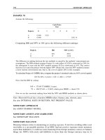
Equation 3 is illustrated in Exhibit 98. The vertical axis shows the percentage appreciation
of the foreign currency relative to the home currency, and the horizontal axis measures the
percentage higher or lower rate of inflation in the foreign country relative to the home country.
Equilibrium is reached on the parity line, which contains all those points at which these two
differentials are equal. At point A, for example, the 3% inflation differential is exactly offset by
the 3% appreciation of the foreign currency relative to the home currency. Point B, on the other
hand, portrays a situation of disparity, where the inflation differential of 3% is greater than the
appreciation of 1% in the home currency value of the foreign currency.
S
2
S
1
1 I
h
+
1 I
f
+

=
S
2
S
1
–
S
1

% change in the foreign currency I
h
I
f
–==
S
2
S
1
–
S
1

I
h
I
f
–
1 I+
h
=
Expected difference in
inflation rates
I
h
I
f
–
1 I+
h

equals
Expected change in spot
rates
S
2
S
1
–
S
1

PURCHASING POWER PARITY (PPP)
SL2910_frame_CP.fm Page 244 Thursday, May 17, 2001 9:10 AM
245
Note: (1) If absolute PPP holds, then relative PPP will also hold. But if absolute PPP does
not hold, relative PPP still may. This is because the level of S may not equal I
f
/I
h
, but the
change in S could still equal the inflation differential. (2) Empirical evidence has indicated
that purchasing power parity holds up well over the long run, but not so well over shorter
time periods.
PURCHASING POWER RISK
Also called inflation risk.
1. The failure of assets (financial and real) to earn a return to keep up with increasing price
levels. Bonds are exposed to this risk because the issuer will be paying back in cheaper
dollars in inflationary times.
2. The domestic counterpart to exchange risk. It involves uncertain changes in the exchange

rate between domestic currency and domestic goods and services.
PUT
1. A right (not the obligation) to sell a specific security at a specified price within a
designated period for which the option buyer pays the seller (writer) a premium or option
price. Contracts on listed puts (and calls) have been standardized at date of issue for
periods of three, six, and nine months, although as these contracts approach expiration,
they may be purchased with a much shorter life.
2. Bondholder’s right to redeem a bond prior to maturity.
PUT OPTION
See PUT.
EXHIBIT 98
Purchasing Power Parity
5
4
3
2
1
-1
-2
-3
-4
-5
1-1-2-3-4-5 2 3 4 5
A
B
Parity line
Inflation differential,
home country relative
to foreign country
Percentage change

in home currency
value of foreign
currency
PUT OPTION
SL2910_frame_CP.fm Page 245 Thursday, May 17, 2001 9:10 AM

246

q

QUANTO

An option in which the foreign exchange risk in the underlying asset has been removed.

QUOTATION

Also

called, quote

.
1. The highest bid to buy and the lowest offer (ask) to sell a security in a particular market
at a given time. For example, a quotation on a stock, say “40 1/4 to 40 3/4,” means that
$40.25 was the highest price any buyer wished to pay (bid) at the time the quotation
was given on the exchange and that $40.75 was the lowest price at which any holder of
the stock offered (asked) to sell.
2. In foreign exchange trading, the pair of prices (bid and ask) at which the dealer is willing
to buy or sell foreign exchange.
See also CURRENCY QUOTATIONS.

SL2910_frame_CQ.fm Page 246 Thursday, May 17, 2001 9:11 AM

247

R

RAND

Monetary unit of Lesotho, South Africa, and South West Africa.

REAL COST OF HEDGING

The real cost of

hedging

is the extra cost of hedging as opposed to not hedging. A

negative

real cost would signify that hedging was more favorable than not hedging.

REAL EXCHANGE RATE

In contrast to

nominal exchange rate

, the rate adjusted for inflation is roughly nominal exchange
rate minus inflation rate.

REGISTERED BOND

A bond registered in the owner’s name and listed on the records of the issuer as well as with
the registrar. Transfer, as at the time of sale or if the bond is being possessed as collateral
for a loan in default, requires power of attorney and the return of the physical bond to a
transfer agent. The transfer agent replaces the old bond with a new one registered to the new
owner. A

bearer bond

is an example of an unregistered bond.

REGRESSION ANALYSIS

Regression analysis is a statistical procedure for estimating mathematically the average
relationship between the dependent variable and the independent variable(

s

).

Simple regres-
sion

involves one independent factor, such as inflation or interest rate differentials, in fore-
casting currency rate, whereas

multiple regression

involves two or more explanatory variables,
e.g., inflation, interest rate differentials, and economic growth together. An example of simple
regression is: A global fund’s return is a function of the return on a world market portfolio,
i.e.,

r

j



=



a



+



br

m

, where

b

=

beta, a measure of uncontrollable risk.

EXAMPLE 107

To explain how beta can be computed, using regression analysis, the data presented in Exhibit 99
is used for an illustrative purpose.

EXHIBIT 99
ABC Global Fund Returns versus EAFE Index Returns

ABC
EAFE Index Returns (%) Global Fund Returns (%)

915
19 20
11 14
14 16
23 25
(

Continued

)

SL2910_frame_CR.fm Page 247 Thursday, May 17, 2001 9:12 AM

248

Exhibit 100 shows MSExcel output for regression analysis.



From the Excel’s regression output, we see:

r

j



=

10.5836

+

0.5632

r

m

which indicates the beta for the particular global fund is 0.5632. It appears that ABC Global
Fund is less risky than the world market, measured by the

EAFE



Index

.

See also FUNDAMENTAL FORECASTING.

REINVOICING CENTER

A central financial facility designated by an MNC to centralize all payments and invoicing
charges subsidiaries fees for its function. This way, it attempts to reduce

transaction exposure

by having all home country exports billed in the home currency and then reinvoiced to each
operating affiliate in that affiliate’s local currency. The reinvoicing center determines which
currencies should be used and where, how, and when. This reinvoicing activity can effectively
shift profits to subsidiaries where tax rates are low.

12 20
12 20
22 23
714
13 22
15 18
17 18

EXHIBIT 100

Summary Output

Regression Statistics

Multiple R 0.7800
R Square 0.6084
Adjusted R Square 0.5692
Standard Error 2.3436
Observations 12.0000

Anova

df SS MS F Significance F

Regression 1 85.3243 85.3243 15.5345 0.0028
Residual 10 54.9257 5.4926
Total 11 140.25

Coefficients
Standard
Error t Stat P-value Lower 95% Upper 95%

Intercept 10.5836 2.1796 4.8558 0.0007 5.7272 15.4401
EAFE Index
Returns
0.5632 0.1429 3.9414 0.0028 0.2448 0.8816

REINVOICING CENTER

SL2910_frame_CR.fm Page 248 Thursday, May 17, 2001 9:12 AM

249

RELATIVE PURCHASING POWER PARITY

See PURCHASING POWER PARITY.

REMBRANDT BONDS

Dutch guilder-denominated bonds issued within the Netherlands by a foreign issuer (bor-
rower).

REPATRIATION

Repatriation is the process of sending cash flows from a foreign subsidiary to the parent
company. Broadly, foreign affiliates make the following payments to the parent company:
(1) dividends, (2) interest and repayment of parent company loans, (3) royalties for use of
trade names and services, (4) management fees for central services, and (5) payments for
goods supplied by the parent. A foreign government may restrict the amount of the cash that
may be repatriated to the parent company. For example, the restriction may be in terms of a
ceiling stated as a percentage of the company’s net worth. Such restrictions are intended to
force multinational companies to reinvest earnings in the foreign country or/and to prevent
large currency outflows, which might disrupt the exchange rate.

REPORTING CURRENCY

The parent company’s currency used in preparing and translating its own financial statements
(e.g., U.S. dollars for a U.S. firm).

REPRESENTATIVE OFFICES

Representative nonbanking offices are established in a foreign country primarily to assist the
parent bank’s customers in that country. Representative offices cannot accept deposits, make
loans, transfer funds, accept drafts, transact in the international money market, or commit
the parent bank to loans. In fact, they cannot cash a traveler’s check drawn on the parent
bank. What they may do, however, is provide information and assist the parent bank’s clients
in their banking and business contacts in the foreign country. For example, a representative
office may introduce business people to local bankers or it may act as an intermediary between
U.S. firms and firms located in the country of the representative office. Of course, while
acting as an intermediary, it provides information about the parent bank’s services. A repre-
sentative’s office is also a primary vehicle by which an initial presence is established in a
country before setting up formal banking operations.

RETURN RELATIVE

It is often necessary to measure returns on a slightly different basis than

total returns (TRs)

.
This is particularly true when calculating a

compound

(or

geometric

)

average return

, because
negative returns cannot be used in the calculation. The return relative (RR) solves this problem
by adding 1.0 to the total return. Although return relatives may be less than 1.0, they will be
greater than zero, thereby eliminating negative numbers.
This can be reduced simply to the following formula (by using the price at the end of the
holding period in the numerator, rather than the

change



in

price):
RR
CP
1
P
0
–()+
P
0
1+=
RR
CP
1

+
P
0
=

RETURN RELATIVE

SL2910_frame_CR.fm Page 249 Thursday, May 17, 2001 9:12 AM

250

EXAMPLE 108

A TR of 0.10 for some holding period is equivalent to a return relative of 1.10, and a TR of

−

0.15 is equivalent to a return relative of 0.85.

See also ARITHEMATIC AVERAGE RETURN VS. COMPOUND (GEOMETRIC) AVER-
AGE RETURN; TOTAL RETURN.

REVALUATION

See CURRENCY REVALUATION.

REVOCABLE LETTER OF CREDIT

A

letter of credit

that the opening bank may revoke at any time without the approval of the
beneficiary. Neither the issuing bank nor the advising and paying bank guarantees payment.

REVOLVING LETTER OF CREDIT

A

letter of credit

which contains a provision for reinstating its face value after being drawn
within a stated period of time facilitates the financing of ongoing regular purchases.

RHO

See CURRENCY OPTION PRICING SENSITIVITY.

RINGGIT

Malaysia’s currency.

RISK

Risk refers to the variation in earnings. It includes the chance of losing money on an
investment. As a measure of risk, we use the standard deviation, which is a statistical measure
of dispersion of the probability distribution of possible returns of an investment. The smaller
the deviation, the tighter the distribution, and thus, the lower the riskiness of the investment.
Mathematically,
To calculate

σ

, we proceed as follows:

Step 1

. First compute the expected rate of return ( )

Step 2

. Subtract each possible return from to obtain a set of deviations

Step 3

. Square each deviation, multiply the squared deviation by the probability of
occurrence for its respective return, and sum these products to obtain the
variance (

σ

)

2

:

Step 4.

Finally, take the square root of the variance to obtain the standard deviation (

σ

).
σ
r
i
r–()
2
p
i
∑
=
r
r r
i
r–()
σ
2
r
1
r–()
2
p
i
∑
=

REVALUATION

SL2910_frame_CR.fm Page 250 Thursday, May 17, 2001 9:12 AM

251

EXAMPLE 109

To follow this step-by-step approach, it is convenient to set up a table, as follows:

Exhibit 103 shows average return rates and standard deviations for selected types of
investments.
The financial manager must be careful in using the standard deviation to compare risk, as
it is only an absolute measure of dispersion (risk). In other words, it does not consider the
risk in relationship to an expected return. In comparisons of securities with differing expected
returns, we commonly use the

coefficient of variation

. The coefficient of variation is computed
simply by dividing the standard deviation for a security by its expected value, i.e.,
The higher the coefficient, the more risky the security.

Return (

r

i

) Probability(

p

i

)
(step 1)

r

i

p

i


(step 2)
(

r

i



−

)
(step 3)
(

r

i



−

)

2

(step 4)
(

r

i



−

)

2

p

i

Stock A

−

5% .2

−

1%

−

24% 576 115.2
20 .6 12 1 1 .6
40 .2

21 441


=

19%

σ

2

=

204


σ



=




=

14.18%

Stock B

10% .2 2%

−

5% 25 5
15 .6 9 0 0 0
20 .2 5 25


=

15%

σ

2



=

10


σ

2



=




σ



=

3.16%

EXHIBIT 103
Risk and Return 1926–1995
Geometric Arithmetic Standard
Series Average Average Deviation
Common stocks 8.81% 10.20% 16.89%
Long-term corporate bonds 5.03 5.58 11.26
Long-term government bonds 4.70 5.11 9.70
U.S. Treasury bills 6.25 6.29 3.10
Source: Ibbotson, R. and Rex A. Sinquefield, Stocks, Bonds, Bills and Inflation: 1996 Year-
book (Chicago: Dow Jones–Irwin, 1996) (www.ibbotson.com/).
r r r
8
88.2
r
204
4
5
r
10
σ
r
⁄
RISK
SL2910_frame_CR.fm Page 251 Thursday, May 17, 2001 9:12 AM
252
EXAMPLE 110
Based on the following data, we can compute the coefficient of variation for each stock as follows:

The coefficient of variation is computed as follows:
For stock A,
For stock B,
Although stock A produces a considerably higher return than stock B, stock A is overall more
risky than stock B, based on the computed coefficient of variation. Note, however, that if
investments have the same expected returns there is no need for the calculation of the coefficient
of determination.
A. Sources of Risk
Different sources of risk are involved in investment and financial decisions. Investors and
decision makers must take into account the type of risk underlying an asset.
1. Financial risk. This is a type of investment risk associated with excessive debt.
2. Industry risk. This risk concerns the uncertainty of the inherent nature of the
industry such as high-technology, product liability, and accidents.
3. International and political risks. These risks stem from foreign operations in polit-
ically unstable foreign countries. An example is a U.S. company having a location
and operations in a hostile country.
4. Economic risk. This is the negative impact of a company from economic slow-
downs. For example, airlines have lower business volume in recession.
5. Currency exchange risk. This risk arises from the fluctuation in foreign exchange rates.
6. Social risk. This is caused by problems facing the company due to ethnic boycott,
discrimination cases, and environmental concerns.
7. Business risk. This is caused by fluctuations of earnings before interest and taxes
(operating income). Business risk depends on variability in demand, sales price,
input prices, and amount of operating leverage.
8. Liquidity risk. It represents the possibility that an asset may not be sold on short
notice for its market value. If an investment must be sold at a high discount, then
it is said to have a substantial amount of liquidity risk.
9. Default risk. It is the risk that a borrower will be unable to make interest payments
or principal repayments on a debt. For example, there is a great amount of default
risk inherent in the bonds of a company experiencing financial difficulty.

10. Market risk. Prices of all stocks are correlated to some degree with broad swings
in the stock market. Market risk refers to changes in a stock’s price that result from
changes in the stock market as a whole, regardless of the fundamental change in
a firm’s earning power.
Stock A Stock B
19% 15%
σ
14.28% 3.16%
r
σ
r⁄ 14.18 19⁄ .75==
σ
r⁄ 3.16 15⁄ .21==
RISK
SL2910_frame_CR.fm Page 252 Thursday, May 17, 2001 9:12 AM