International Macroeconomics and Finance: Theory and Empirical Methods Phần 5 docx
Bạn đang xem bản rút gọn của tài liệu. Xem và tải ngay bản đầy đủ của tài liệu tại đây (498.86 KB, 38 trang )
5.1. CALIBRATING THE ONE-SECTOR GROWTH MODEL 145
where a
0
= U
c
g
1
+ βU
c
g
2
=0,
a
1
= βU
cc
g
1
g
2
,
a
2
= U
cc
g
2
1
+ βU
cc
g
2
2
+ βU
c
g
22
,
a
3
= U
cc
g
1
g
2
,
a
4
= βU
c
g
32
+ βU
cc
g
2
g
3
,
a
5
= U
cc
g
1
g
3
.
The derivatives are evaluated at steady state values.
A second but equivalent option is to take a second—order Taylor
approximation to the objective function around the steady state and to
solve the resulting quadratic optimi zation problem. The second o ption
is equivalent to the Þrst because it yields linear Þrst—order conditions
around the steady state. To pursue the second option, recall that λ
t
=
(k
t+1
,k
t
,A
t
)
0
. Write the period utility function in the unconstrained
optimization problem as
R(λ
t
)=U[g(λ
t
)]. (5.20)
Let R
j
= ∂R(λ
t
)/∂λ
jt
be the partial derivative of R(λ
t
) with respect
to the j−th element of λ
t
and R
ij
= ∂
2
R(λ
t
)/(∂λ
it
∂λ
jt
) be the second
cross-partial derivative. Since R
ij
= R
ji
the relevant derivatives are,
R
1
= U
c
g
1
,
R
2
= U
c
g
2
,
R
3
= U
c
g
3
,
R
11
= U
cc
g
2
1
,
R
22
= U
cc
g
2
2
, +U
c
g
22
R
33
= U
cc
g
2
3
,
R
12
= U
cc
g
1
g
2
,
R
13
= U
cc
g
1
g
3
,
R
23
= U
cc
g
2
g
3
+ U
c
g
23
.
The second-order Taylor expansion of the period utility function is
R(λ
t
)=R(λ)+R
1
(k
t+1
− k)+R
2
(k
t
− k)+R
3
(A
t
− A)+
1
2
R
11
(k
t+1
− k)
2
146 CHAPTER 5. INTERNATIONAL REAL BUSINESS CYCLES
+
1
2
R
22
(k
t
− k)
2
+
1
2
R
33
(A
t
− A)
2
+ R
12
(k
t+1
− k)(k
t
− k)
+R
13
(k
t+1
− k)(A
t
− A)+R
23
(k
t
− k)(A
t
− A).
Suppose we let q =(R
1
,R
2
,R
3
)
0
be the 3 × 1 row vector of partial
derivatives (the gradient) of R,andQ be the 3 × 3matrixofsecond
partial derivatives (the Hessian) multiplied by 1/2whereQ
ij
= R
ij
/2.
Then the approximate period utility function can be compactly written
in matrix form as
R(λ
t
)=R(λ)+[q +(λ
t
− λ)
0
Q](λ
t
− λ). (5.21)
The problem is now to maximize
E
t
∞
X
j=0
β
j
R(λ
t+j
). (5.22)
The Þrst order conditions are for all t
0=(βR
2
+ R
1
)+βR
12
(k
t+2
− k)+(R
11
+ βR
22
)(k
t+1
− k)+R
12
(k
t
− k)
+βR
23
(A
t+1
− 1) + R
13
(A
t
− 1). (5.23)
If you compare (5.23) to (5.19), you’ll see that a
0
= βR
2
+ R
1
,
a
1
= βR
12
,a
2
= R
11
+ βR
22
,a
3
= R
12
,a
4
= βR
23
,a
5
= R
13
.This
veriÞes that the two approaches are indeed equivalent.
Now to solve the linearized Þrst-order conditions, work with (5.19).
Since the data that we want to explain are in logarithms, you can con-
vert the Þrst-order cond itions into near logarithmic form. Let
˜a
i
= ka
i
for i =1, 2, 3, and let a “hat” denote the approximate log
difference from the steady state so that
ˆ
k
t
=(k
t
− k)/k ' ln(k
t
/k)
and
ˆ
A
t
= A
t
− 1 (since the steady state value of A =1). Nowlet
b
1
= −˜a
2
/˜a
1
, b
2
= −˜a
3
/˜a
1
, b
3
= −a
4
/˜a
1
, and b
4
= −a
4
/˜a
1
.
The second—order stochastic difference equation (5.19) can be writ-
ten as
(1 − b
1
L − b
2
L
2
)
ˆ
k
t+1
= W
t
, (5.24)
where
W
t
= b
3
ˆ
A
t+1
+ b
4
ˆ
A
t
.
5.1. CALIBRATING THE ONE-SECTOR GROWTH MODEL 147
The roots of the polynomial (1 − b
1
z − b
2
z
2
)=(1− ω
1
L)(1 − ω
2
L)
satisf y b
1
= ω
1
+ ω
2
and b
2
= −ω
1
ω
2
. Using the quadratic formula
and evaluating at the parameter values that we used to calibrate the
model, the roots are, z
1
=(1/ω
1
)=[−b
1
−
q
b
2
1
+4b
2
]/(2b
2
) ' 1.23, and
z
2
=(1/ω
2
)=[−b
1
+
q
b
2
1
+4b
2
]/(2b
2
) ' 0.81. There is a stable root,
|z
1
| > 1 which lies outside the unit circle, and an unstable root, |z
2
| < 1
which lies inside the unit circle. The presence of an unstable root means
that the solution is a saddle path. If you try to simulate (5.24) directly,
the capital stock will diverge.
To solve the difference equation, exploit the certainty equivalence
property of quadratic optimization problems. That is, you Þrst get
the perfect foresight solution to the problem by solving the stable root
backwards and the unstable root forwards. Then, replace future ran-
dom variables with their expected values conditional upon the time-t
information set. Begin by rewriting (5.24) as
W
t
=(1− ω
1
L)(1 − ω
2
L)
ˆ
k
t+1
=(−ω
2
L)(−ω
−1
2
L
−1
)(1 − ω
2
L)(1 − ω
1
L)
ˆ
k
t+1
=(−ω
2
L)(1 − ω
−1
2
L
−1
)(1 − ω
1
L)
ˆ
k
t+1
,
and rearrange to get
(1 − ω
1
L)
ˆ
k
t+1
=
−ω
−1
2
L
−1
1 − ω
−1
2
L
−1
W
t
= −
µ
1
ω
2
L
−1
∞
X
j=0
µ
1
ω
2
j
W
t+j
= −
∞
X
j=1
µ
1
ω
2
j
W
t+j
. (5.25)
The autoregressive speciÞcation (5.18) implies the prediction formulae
E
t
W
t+j
= b
3
E
t
ˆ
A
t+j+1
+ b
4
E
t
ˆ
A
t+j
=[b
3
ρ + b
4
]ρ
j
ˆ
A
t
.
Use this forecasting rule in (5.25) to get
∞
X
j=1
µ
1
ω
2
j
E
t
W
t+j
=[b
3
ρ + b
4
]
ˆ
A
t
∞
X
j=1
µ
ρ
ω
2
j
=
"
ρ
ω
2
− ρ
#
(b
3
ρ + b
4
)
ˆ
A
t
.
148 CHAPTER 5. INTERNATIONAL REAL BUSINESS CYCLES
It follows that the solution for the capital stock is
ˆ
k
t+1
= ω
1
ˆ
k
t
−
"
ρ
ω
2
− ρ
#
[b
3
ρ + b
4
]
ˆ
A
t
. (5.26)
To recover ˆy
t
, note that the Þrst-order expansion of the produc-
tion function gives y
t
= f(A, k)+f
A
ˆ
A
t
+ f
k
k
ˆ
k
t
,wheref
A
=1, and
f
k
=(αy)/k. Rearrangement gives ˆy
t
=
ˆ
A
t
+
ˆ
k
t
.Torecover
ˆ
i
t
, subtract
the steady state value γk = i +(1−δ)k from (5.8) and rearrange to get
ˆ
i
t
=(k/i)[γ
ˆ
k
t+1
−(1−δ)
ˆ
k
t
]. Finally, get ˆc
t
=ˆy
t
−
ˆ
i
t
from the adding-up
constraint (5.9). The log levels of the variables can be recovered by
ln(Y
t
)=ˆy
t
+ln(X
t
)+ln(y),
ln(C
t
)=ˆc
t
+ln(X
t
)+ln(c),
ln(I
t
)=
ˆ
i
t
+ln(X
t
)+ln(i),
ln(X
t
)=ln(X
0
)+t ln(γ).
Sim u lating the Model
We’ll use the calibrated model to generate 96 time-series observations
corresponding to the n umber of observations in the data. From these
pseudo-observations, recover the implied log-levels and pass them through
the Hodrick-Prescott Þlter. The steady state values are
y =1.717,k=5.147,c=1.201,i/k=0.10.
Plots of the Þltered log income, consumption, and investmen t o bserva-
tions are given in Figure 5.3 and the associated descriptive statistics are
given in Table 5.2. The autoregressive coefficien t and the error variance
of the technology shock were selected to match the volatility of output
exactly. From the Þgure, you can see that both consumption and in-
vestment exhibit high co-movemen ts w ith output, and all three series
display persistence. However from Table 5.2 the implied inv estment
series is seen to be more volatile than output but is less v olatile than
that found in the data. Consumption implied by the model is more
volatile than output, which is counterfactual.
5.2. CALIBRATING A TWO-COUNTRY MODEL 149
-0.2
-0.15
-0.1
-0.05
0
0.05
73 75 77 79 81 83 85 87 89 91 93 95
Investment
GDP (broken)
Consumption
Figure 5.3: Hodrick-Presco tt Þltered cyclical observations from the
model. Investment has been shifted down b y 0.10 for visual clarity.
This coarse overview of the one sector real business cycle model
shows that there are some aspects of the data that the model does not
explain. This is not surprising. Perhaps it is more surprising is how
well it actually does in generating ‘realistic’ time series dynamics of the
data. In any event, this perfect markets—no nominal rigidities Arrow-
Debreu model serves as a useful benchmark against which reÞnements
can be judged.
5.2 Calibrating a Two-Country Model
We now add a second country. This two-country model is a special
case of Backus et. al. [5]. Each county produces the same good so we
will not be able to study terms of trade or real exchange rate issues.
The presence of country-speciÞc idiosyncratic shocks give an incentive
to individuals in the two countries to trade as a means to insure each
150 CHAPTER 5. INTERNATIONAL REAL BUSINESS CYCLES
Table 5.2: Calibrated Closed-Economy Model
Std. Autocorrelations
Dev. 1 2 3 4 6
y
t
0.022 0.90 0.79 0.67 0.53 0.23
c
t
0.023 0.97 0.89 0.77 0.63 0.31
i
t
0.034 0.70 0.50 0.36 0.19 -0.04
Cross correlation with y
t−k
at k
6 4 1 0 -1 -4 -6
c
t
0.49 0.77 0.96 0.90 0.79 0.33 0.04
i
t
0.29 0.11 0.41 0.74 0.73 0.61 0.44
other against a bad relative technology shock so we can examine the
behavior of the current account.
Measurement
We will call the Þrst c ountry the ‘US,’ and second country ‘Europe.’
The data for European output, government spending, investment, and
consumption are the aggregate of observations for the U K, France, Ger-
many, and Italy. The aggregate of their current account balances suf-
fer from double counting and does not make sense because of intra-
European trade. Therefore, we examine only the US current account,
which is measured as a fraction of real GDP.
Table 5.3 displays the features of the data that we will attempt to
explain–their volatility, persistence (characterized by their autocorre-
lations) and their co-movements (characterized by cross correlations).
Notice that US and European consumption correlation is lower than
the their output correlation.
The Two-Country Model
Both countries experience identical rates of depreciation of phy sical
capital, long-run technological growth X
t+1
/X
t
= X
∗
t+1
/X
∗
t
= γ,have
5.2. CALIBRATING A TWO-COUNTRY MODEL 151
Table 5.3: Open-Economy Measurements
Std. Autocorrelations
Dev. 1 2 3 4 6
ex
t
0.01 0.61 0.50 0.40 0.40 0.12
y
∗
t
0.014 0.84 0.62 0.36 0.15 -0.15
c
∗
t
0.010 0.68 0.47 0.30 0.04 -0.15
i
∗
t
0.030 0.89 0.75 0.57 0.40 0.07
Cross correlations at lag k
6 4 1 0 -1 -4 6
y
t
ex
t−k
0.43 0.42 0.41 0.41 0.37 0.03 0.32
y
t
y
∗
t−k
0.28 0.22 0.21 0.36 0.43 0.36 0.22
c
t
c
∗
t−k
0.26 0.39 0.28 0.25 0.05 0.15 0.26
Notes: ex
t
is US net exports divided by GDP. Foreign country aggregates data from
France, Germany, Italy, and the UK. All variables are real per capita from 1973.1
to 1996.4 and have been passed through the Hodrick—Prescott Þlter with λ = 1600.
the same capital shares and Cobb-Douglas form of the production func-
tion, and identical utility. Let the social planner attach a weight of ω to
the domestic agent and a weight of 1−ω to the foreign agent. In terms
of efficiency units, the social planner’s problem is now to maximize
E
t
∞
X
j=0
β
j
[ωU(c
t+j
)+(1− ω)U(c
∗
t+j
)], (5.27)
subject to,
y
t
= f(A
t
,k
t
)=A
t
k
α
t
, (5.28)
y
∗
t
= f(A
∗
t
,k
∗
t
)=A
∗
t
k
∗α
t
, (5.29)
γk
t+1
= i
t
+(1− δ)k
t
, (5.30)
γk
∗
t+1
= i
∗
t
+(1− δ)k
∗
t
, (5.31)
y
t
+ y
∗
t
= c
t
+ c
∗
t
+(i
t
+ i
∗
t
). (5.32)
In the market economy interpretation, we can view ω to indicate the
size of the home country in the world economy. (5.28) and (5.29) are the
152 CHAPTER 5. INTERNATIONAL REAL BUSINESS CYCLES
Cobb—Douglas production functions for the home and foreign counties,
with normalized labor input N = N
∗
= 1. (5.30) and (5.31) are the
domestic and foreign capital accumulation equations, and (5.31) is the
new form of the resource constraint. Both countries have the same
technology but are subject to heterogeneous transient shocks to total
productivity according to
"
A
t
A
∗
t
#
=
"
1 − ρ − δ
1 − ρ − δ
#
+
"
ρδ
δρ
#"
A
t−1
A
∗
t−1
#
+
"
²
t
²
∗
t
#
, (5.33)
where (²
t
,²
∗
t
)
0
iid
∼ N(0, Σ). We set ρ =0.906, δ =0.088, Σ
11
= Σ
22
=
2.40e−4, and Σ
12
= Σ
21
=6.17e−5. The contemporaneous correlation
of the innovations is 0.26.
Apart from the objective function, the main difference between the
two-county and one-country models is the resource constraint (5.32).
World output can either be consumed or sav ed but a country’s net sav-
ing, which is t he current account balance, can be non—zero
(y
t
− c
t
− i
t
= −(y
∗
t
− c
∗
t
− i
∗
t
) 6=0).
Let λ
t
=(k
t+1
,k
∗
t+1
,k
t
,k
∗
t
,A
t
,A
∗
t
,c
∗
t
) be the state vector, and i ndi-
cate the dependence of consumption on the state by c
t
= g(λ
t
), and
c
∗
t
= h(λ
t
)(whichequalsc
∗
t
trivially). Substitute (5.28)—(5.31) into
(5.32) and re-arrange to get
c
t
= g(λ
t
)=f(A
t
,k
t
)+f(A
∗
t
,k
∗
t
) − γ(k
t+1
+ k
∗
t+1
),
+(1 − δ)(k
t
+ k
∗
t
) − c
∗
t
(5.34)
c
∗
t
= h(λ
t
)=c
∗
t
. (5.35)
For future referen ce, the derivatives of g and h are,
g
1
= g
2
= −γ,
g
3
= f
k
(A, k)+(1− δ),
g
4
= f
k
(A
∗
,k
∗
)+(1− δ),
g
5
= f(A, k)/A,
g
6
= f(A
∗
,k
∗
)/A
∗
,
g
7
= −1,
h
1
= h
2
= ···= h
6
=0,
h
7
=1.
5.2. CALIBRATING A TWO-COUNTRY MODEL 153
Next, transform the constrained optimization problem into an un-
constrained problem by substituting (5.34) and (5.35) into (5.27). The
problem is now to maximize
ωE
t
³
u[g(λ
t
)] + βU[g(λ
t+1
)] + β
2
U[g (λ
t+2
)] + ···
´
(5.36)
+(1 −ω)E
t
³
u[h(λ
t
)] + βU[h(λ
t+1
)] + β
2
U[h(λ
t+2
)] + ···
´
.
At date t, the choice variables available to the planner are k
t+1
,k
∗
t+1
,
and c
∗
t
.Differentiating (5.36) with respect to these variables and re-
arranging results in the Euler equations
γU
c
(c
t
)=βE
t
U
c
(c
t+1
)[g
3
(λ
t+1
)], (5.37)
γU
c
(c
t
)=βE
t
U
c
(c
t+1
)[g
4
(λ
t+1
)], (5.38)
U
c
(c
t
)=[(1− ω)/ω]U
c
(c
∗
t
). (5.39)
(5.39) is the Pareto—Optimal risk sharing rule which sets home marginal
utility proportional to foreign marginal utility. Under log utility, home
and foreign per capita consumption are perfectly correlated,
c
t
=[ω/(1 − ω)]c
∗
t
.
The Two-Country Steady State
From (5.37) and (5.38) we obtain y/k = y
∗
/k
∗
=(γ/β+δ−1)/α.We’ve
already determined that c =[ω/(1 − ω)]c
∗
= ωc
w
where c
w
= c + c
∗
is world consumption. From the production functions (5.28)—(5.29) we
get k =(y/k)
1/(α−1)
and k
∗
=(y
∗
/k
∗
)
1/(α−1)
. From (5.30)—(5.31) we
get i = i
∗
=(γ + δ −1)k. It follows that c = ωc
w
= ω[y + y
∗
−(i + i
∗
)]
=2ω [y − i].
Thus y − c − i =(1− 2ω)(y − i) and unless ω =1/2, the current
account will not be balanced in the steady state. If ω > 1/2thehome
country spends in excess of GDP and runs a current account deÞcit.
How can this be? In the market (competitive equilibrium) interpreta-
tion, the excess absorption is Þnanced by interest income earned on past
lending to the foreign country. Foreigners need to produce in excess of
their consumption and investment to service the debt. In a sense, they
ha ve ‘o ver-invested’ in ph ysical capital.
In the planning problem, the social planner simply takes away some
of the foreign output and gives it to domestic agents. Due to the
154 CHAPTER 5. INTERNATIONAL REAL BUSINESS CYCLES
concavity of the production function, optimality requires that the world
capital stock be split up between the two countries so as to equate the
marginal product of capital at home and abroad. Since technology is
identical in the 2 countries, this implies e qualization of national capital
stocks, k = k
∗
, and income levels y = y
∗
, even if consumption differs,
c 6= c
∗
.
Quadratic Approximation
You can solve the model by taking the quadratic approximation of the
unconstrained objective function about the steady state. Let R be the
period weighted average of home and foreign utility
R(λ
t
)=ωU[g(λ
t
)] + (1 − ω)U[h(λ
t
)].
Let R
j
= ωU
c
(c)g
j
+(1− ω)U
c
(c
∗
)h
j
, j =1, ,7betheÞrst partial
derivative of R with respect to the j−the e lement of λ
t
.Denotethe
second partial derivative of R by
R
jk
=
∂R(λ)
∂λ
j
∂λ
k
= ω[U
c
(c)g
jk
+U
cc
g
j
g
k
]+(1−ω)[U
c
(c
∗
)h
jk
+U
cc
(c
∗
)h
j
h
k
].
(5.40)
Let q =(R
1
, ,R
7
)
0
be the gradient vector, Q be the Hessian matrix
of second partial derivatives whose j, k−th element is Q
jk
=(1/2)R
j,k
.
Then the second-order Taylor approximation to the period utility func-
tion is
R(λ
t
)=[q +(λ
t
− λ)
0
Q](λ
t
− λ),
and you can rewrite (5.36) as
max E
t
∞
X
j=0
β
j
[q +(λ
t+j
− λ)
0
Q](λ
t+j
− λ). (5.41)
Let Q
j•
be the j−th row of the matrix Q.TheÞrst-order conditions
are
(k
t+1
): 0=R
1
+ βR
3
+ Q
1•
(λ
t
− λ)+βQ
3•
(λ
t+1
− λ), (5.42)
(k
∗
t+1
): 0=R
2
+ βR
4
+ Q
2•
(λ
t
− λ)+βQ
4•
(λ
t+1
λ), (5.43)
(c
∗
t
): 0=R
7
+ Q
7•
(λ
t
− λ). (5.44)
5.2. CALIBRATING A TWO-COUNTRY MODEL 155
Now let a ‘tilde’ denote the deviation of a variable from its steady state
value so that
˜
k
t
= k
t
− k and write these equations out as
0=a
1
˜
k
t+2
+ a
2
˜
k
∗
t+2
+ a
3
˜
k
t+1
+ a
4
˜
k
∗
t+1
+ a
5
˜
k
t
+ a
6
˜
k
∗
t
+ a
7
˜
A
t+1
+a
8
˜
A
∗
t+1
+ a
9
˜
A
t
+ a
10
˜
A
∗
t
+ a
11
˜c
∗
t+1
+ a
12
˜c
∗
t
+ a
13
, (5.45)
0=b
1
˜
k
t+2
+ b
2
˜
k
∗
t+2
+ b
3
˜
k
t+1
+ b
4
˜
k
∗
t+1
+ b
5
˜
k
t
+ b
6
˜
k
∗
t
+ b
7
˜
A
t+1
+b
8
˜
A
∗
t+1
+ b
9
˜
A
t
+ b
10
˜
A
∗
t
+ b
11
˜c
∗
t+1
+ b
12
˜c
∗
t
+ b
13
, (5.46)
0=d
3
˜
k
t+1
+ d
4
˜
k
∗
t+1
+ d
5
˜
k
t
+ d
6
˜
k
∗
t
+ d
9
˜
A
t
+ d
10
˜
A
∗
t
+d
12
˜c
∗
t
+ d
13
, (5.47)
where the coefficients are given by
j a
j
b
j
d
j
1 βQ
31
βQ
41
0
2 βQ
32
βQ
42
0
3 βQ
33
+ Q
11
βQ
43
+ Q
21
Q
71
4 βQ
34
+ Q
12
βQ
44
+ Q
22
Q
72
5 Q
13
Q
23
Q
73
6 Q
14
Q
24
Q
74
7 βQ
35
βQ
45
0
8 βQ
36
βQ
46
0
9 Q
15
Q
25
Q
75
10 Q
16
Q
26
Q
76
11 Q
37
Q
47
0
12 Q
17
Q
27
Q
77
13 R
1
+ βR
3
R
2
+ βR
4
R
7
Mimicking the algorithm developed for the one-country model and
using (5.47) to substitute out c
∗
t
and c
∗
t+1
in (5.45) and (5.46) gives
0=˜a
1
˜
k
t+2
+˜a
2
˜
k
∗
t+2
+˜a
3
˜
k
t+1
+˜a
4
˜
k
∗
t+1
+˜a
5
˜
k
t
+˜a
6
˜
k
∗
t
+˜a
7
˜
A
t+1
+˜a
8
˜
A
∗
t+1
+˜a
9
˜
A
t
+˜a
10
˜
A
∗
t
+˜a
11
, (5.48)
0=
˜
b
1
˜
k
t+2
+
˜
b
2
˜
k
∗
t+2
+
˜
b
3
˜
k
t+1
+
˜
b
4
˜
k
∗
t+1
+
˜
b
5
˜
k
t
+
˜
b
6
˜
k
∗
t
+
˜
b
7
˜
A
t+1
+
˜
b
8
˜
A
∗
t+1
+
˜
b
9
˜
A
t
+
˜
b
10
˜
A
∗
t
+
˜
b
11
. (5.49)
156 CHAPTER 5. INTERNATIONAL REAL BUSINESS CYCLES
At this point, the marginal beneÞt from looking at analytic expressions
for the coefficients is probably nega tive. For the speci Þc calibration of
the model the numerical va lues of the coefficients are,
˜a
1
=0.105,
˜
b
1
=0.105,
˜a
2
=0.105,
˜
b
2
=0.105,
˜a
3
= −0.218,
˜
b
3
= −0.212,
˜a
4
= −0.212,
˜
b
4
= −0.218,
˜a
5
=0.107,
˜
b
5
=0.107,
˜a
6
=0.107,
˜
b
6
=0.107,
˜a
7
= −0.128,
˜
b
7
= −0.161,
˜a
8
= −0.159,
˜
b
8
= −0.130,
˜a
9
=0.158,
˜
b
9
=0.158,
˜a
10
=0.158,
˜
b
10
=0.158,
˜a
11
=0.007,
˜
b
11
=0.007.
You can see that ˜a
3
+˜a
4
=
˜
b
3
+
˜
b
4
and ˜a
7
+
˜
b
7
=˜a
8
+
˜
b
8
which means
that there is a singularity in this system. To deal with this singularity,
let
˜
A
w
t
=
˜
A
t
+
˜
A
∗
t
denote the ‘world’ technology shock and add (5.48)
to (5.49) to get
˜a
1
˜
k
w
t+2
+
˜a
3
+˜a
4
2
˜
k
w
t+1
+˜a
5
˜
k
w
t
+
˜a
7
+
˜
b
7
2
˜
A
w
t+1
+˜a
9
˜
A
w
t
+
˜a
11
+
˜
b
11
2
=0. (5.50)
(5.50) is a second—order stochastic difference equation in
˜
k
w
t
=
˜
k
t
+
˜
k
∗
t
,
which can be rewritten compactly as
4
˜
k
w
t+2
− m
1
˜
k
w
t+1
− m
2
˜
k
w
t
= W
w
t+1
, (5.51)
where W
w
t+1
= m
3
˜
A
w
t+1
+ m
4
˜
A
w
t
,and
m
1
= −(˜a
3
+˜a
4
)/(2˜a
1
),
m
2
= −˜a
5
/˜a
1
,
m
3
= −(˜a
7
+
˜
b
7
)/(2˜a
1
),
m
4
= −˜a
9
/˜a
1
,
m
5
= −
˜a
11
+
˜
b
11
2˜a
11
.
4
Unlike the one-country model, we don’t want to write the model in logs because
we have to be able to recover
˜
k and
˜
k
∗
separately.
5.2. CALIBRATING A TWO-COUNTRY MODEL 157
You can write second—order stochastic difference equation (5.51) as
(1 − m
1
L − m
2
L
2
)
ˆ
k
w
t+1
= W
w
t
. The roots of the polynomial
(1 −m
1
z −m
2
z
2
)=(1−ω
1
L)(1 −ω
2
L) satisfy m
1
= ω
1
+ ω
2
and m
2
=
−ω
1
ω
2
. Under the parameter values used to calibrate the model and us-
ing the quadratic formula, the roots are, z
1
=(1/ω
1
)=
[−m
1
−
q
m
2
1
+4m
2
]/(2m
2
) ' 1.17, and z
2
=(1/ω
2
)=
[−m
1
+
q
m
2
1
+4m
2
]/(2m
2
) ' 0.84. The stable root |z
1
| > 1 lies outside
the unit circle, and t he unstable roo t |z
2
| < 1 lies i nside the unit circle.
From the law of motion governing the technology shocks (5.33), you
hav e
˜
A
w
t+1
=(ρ + δ)
˜
A
w
t
+ ²
w
t
, (5.52)
where ²
w
t
= ²
t
+ ²
∗
t
.NowE
t
W
t+k
= m
3
˜
A
w
t+1
+ m
4
˜
A
w
t
+ m
5
=
[m
3
(ρ + δ)+m
4
](ρ + δ)
k
˜
A
w
t
+ m
5
. As in the one-country model, use
these forecasting formulae to solve the unstable root forwards and the
stable root backwards. The solution for the world capital stock is
˜
k
w
t+1
= ω
1
˜
k
w
t
−
(ρ + δ)
ω
2
− (ρ + δ)
³
[m
3
(ρ + δ)+m
4
]
˜
A
w
t
+ m
5
´
. (5.53)
Now you need to recover the domestic and foreign components of
the world capital stock. Subtract (5.49) from (5.48) to get
˜
k
t+1
−
˜
k
∗
t+1
=
Ã
˜
b
7
− ˜a
7
˜a
3
− ˜a
4
!
˜
A
t+1
+
Ã
˜
b
8
− ˜a
8
˜a
3
− ˜a
4
!
˜
A
∗
t+1
. (5.54)
Add (5.53) to (5.54) to get
˜
k
t+1
=
1
2
[
˜
k
w
t+1
+(
˜
k
t+1
−
˜
k
∗
t+1
)]. (5.55)
The d ate t +1 world capital stock is predetermined at date t.Howthat
capital is allocated between the home and foreign country depends on
the realization of the idiosyncratic shocks
˜
A
t+1
and
˜
A
∗
t+1
.
Given
˜
k
t
,and
˜
k
∗
t
, it follows from the production functions that the
outputs are
˜y
t
= f
A
˜
A
t
+ f
k
˜
k
t
= y
˜
A
t
+ α
y
k
˜
k
t
, (5.56)
˜y
∗
t
= f
∗
A
˜
A
∗
t
+ f
∗
k
˜
k
∗
t
= y
∗
˜
A
∗
t
+ α
y
∗
k
∗
˜
k
∗
t
, (5.57)
158 CHAPTER 5. INTERNATIONAL REAL BUSINESS CYCLES
and investment rates are
˜
i
t
= γ
˜
k
t+1
− (1 − δ)
˜
k
t
, (5.58)
˜
i
∗
t
= γ
˜
k
∗
t+1
− (1 − δ)
˜
k
∗
t
. (5.59)
Let world consumption be ˜c
w
t
=˜c
t
+˜c
∗
t
=˜y
t
+˜y
∗
t
− (
˜
i
t
+
˜
i
∗
t
). By the
optimal risk-sharing rule (5.39) ˜c
∗
t
=[(1− ω)/ω]˜c
t
,whichcanbeused
to determine
˜c
t
= ω˜c
w
t
. (5.60)
It follows that ˜c
∗
t
=˜c
w
t
− ˜c
t
. The log-level of consumption is recovered
by
ln(C
t
)=ln(X
t
)+ln(˜c
t
+ c).
Log levels of the other variables can be obtained in an analogous man-
ner.
Simulating the Two-Country Model
The steady state values are
y = y
∗
=1.53,k= k
∗
=3.66,i= i
∗
=0.42,c= c
∗
=1.11.
The model is used to generate 96 time-series observations. Descriptive
statistics calculated using the Hodrick—Prescott Þltered cyclic al parts of
the log-levels of the simulated observations and are displayed in Table
5.4 and Figure 5.4 sho ws the simulated current account balance.
The simple model of this chapter makes many realistic predictions.
It produce s time-series that are persistent and that display coarse co-
movements that a re broadly consistent with the data. But there are
also several features of the model that are inconsistent with the data.
First, consumption in the two-country model is smoother than output.
Second, domestic and foreign consumption are perfectly correlated due
to the perfect risk-sharing whereas the correlation in the data is much
lower than 1. A related point is that home and foreign output are
predicted to display a lower degree of co-mo vement than home and
foreign consumption which also is not borne out in the data.
5.2. CALIBRATING A TWO-COUNTRY MODEL 159
-0.1
-0.08
-0.06
-0.04
-0.02
0
0.02
0.04
0.06
0.08
0.1
73 75 77 79 81 83 85 87 89 91 93 95 97
Figure 5.4: Simulated current account to GDP ratio.
Table 5.4: Calibrated Open-Economy Model
Std. Autocorrelations
Dev. 1 2 3 4 6
y
t
0.022 0.66 0.40 0.15 0.07 0.04
c
t
0.017 0.63 0.42 0.18 0.12 -0.04
i
t
0.114 0.05 -0.13 -0.09 -0.10 0.03
ex
t
0.038 0.09 -0.09 -0.09 -0.10 -0.00
y
∗
t
0.021 0.65 0.32 0.07 -0.15 -0.27
c
∗
t
0.017 0.63 0.42 0.18 0.12 -0.04
i
∗
t
0.116 0.03 -0.15 -0.07 -0.08 0.00
Cross correlations at k
6 4 1 0 -1 -4 -6
ex
t
y
t−k
0.00 0.18 0.41 0.44 0.2 1 0.15 0.15
y
∗
t
y
t−k
0.10 0.06 0.27 0.18 0.0 6 0.28 0.05
160 CHAPTER 5. INTERNATIONAL REAL BUSINESS CYCLES
In ternational R eal Business Cycles Summary
1. The workhorse of real business cycle research is the dynamic
stochastic general equilibrium model. These can be viewed as
Arrow-Debreu models and solved by exploiting the social plan-
ner’s problem. They feature perfect markets and completely
fully ßexible prices . The models are fully articulated and are
have solidly grounded micro foundations.
2. Real business cycle researchers employ the calibration method to
quantitatively evaluate their models. Typically, the researcher
takes a set of moments such as correlations between actual time
series, and asks if the theory is capable of replicating these co-
movements. The calibration style of research stands in contrast
with econometric methodology as articulated in the Cowles com-
mission tradition. In standard econometric practice one begins
by achieving model identiÞcation, progressing to estimation of
the structural parameters, and Þnally by conducting hypothesis
tests of the model’s overidentifying restrictions but how one de-
termines whether the model is successful or not in the calibration
tradition is not entirely clear.
Chapter 6
Foreign Exchange Market
Efficiency
In his second review article on efficient capital markets, Fama [49]
writes,
“I take the market efficiency hypothesis to be the sim-
ple statement that security prices fully reßect all available
information.”
He goes on to say,
“. . . , market efficiency per se i s not testable. I t must
be tested jointly with some model of equilibrium, an asset-
pricing mo del.”
Market efficiency does not mean that asset returns are serially un-
correlated,nordoesitmeanthattheÞnancial markets present zero
expected proÞts. The crux of market efficiency is that there are no
unexploited excess proÞt opportunities. What is considered to be ex-
cessive depend s on the model of market equilibrium.
This chapter is an introduction to the economics of foreign exchange
market efficiency. We begin with an evaluation of the simplest model of
international currency and money-market eq uilibrium–uncovered in-
terest parity. Econometric analyses show that it is strongly rejected by
161
162CHAPTER 6. FOREIGN EXCHANGE MARKET EFFICIENCY
the data. The ensuing challenge is then to understand why uncovered
interest parity fails.
We cove r three possible explanations. The Þrst is that the for-
ward foreign exchange rate contains a risk premium. This argument
is developed using the Lucas model of chapter 4. The second explana-
tion is that the true underlying structure of the economy is subject to
change o ccasionally but economic agents only learn about these struc-
tural changes over time. During this transitional learning period in
which market participants have an incomplete understanding of the
economy and make systematic prediction errors even though they are
behaving rationally. This is called the ‘peso-problem’ approach. The
third explanation is that some market participants are actually irra-
tional in the sense that they believe that the value of an asset depends
on extraneous information in addition to the economic fundamentals.
The individuals who take actions based on these pseudo signals are
called ‘noise’ traders.
The notational convention followed in this chapter is to let upper
case letters denote variables in levels and lower case letters denote their
logarithms, with the exception of interest rates, which are alway s de-
noted in lower case. As usual, stars are used to denote foreign country
variables.
6.1 Deviations From UIP
Let s be the log spot exchange rate, f be the log one-period forward
rate, i be the one-period nominal interest rate on a domestic currency
(dollar) asset and i
∗
is the nominal interest rate on the foreign currency
(euro) asset. If uncovered in terest parity holds, i
t
− i
∗
t
=E
t
(s
t+1
) − s
t
,
but by covered interest parit y, i
t
−i
∗
t
= f
t
−s
t
. Therefore, unbiasedness
of the forward exchange rate as a predictor of the future spot rate
f
t
=E
t
(s
t+1
) is equivalent to uncovered interest parity.
We begin by covering the basic econome tric analyses used to detect
these deviations.
6.1. DEVIATIONS FROM UIP 163
Hansen and Hodrick ’s Tests of UIP
Hansen and Hodrick [71] use generalized method of moments (GMM)
to test uncovered interest parity. The GMM method is covered in
chapter 2.2. The Hansen—Hodrick problem is that a moving-average se-
rial correlation is induced into the regression error when the prediction
horizon exceeds the sampling interval of the data.
The Hansen—Ho drick Problem
Toseehowtheproblemarises,letf
t,3
be the log 3-month forward ex-
change rate at time t, s
t
be the log spot rate, I
t
be the time t information ⇐(102)
setavailabletomarketparticipants,andJ
t
be the time t information
set available to you, the econometrician. Even though you are working
with 3-month forward rates, you will sample the data monthly. You
want to test the hypothesis
H
0
:E(s
t+3
|I
t
)=f
t,3
.
In setting up the test, you note that I
t
is not observable but since J
t
is
asubsetofI
t
and since f
t,3
is contained in J
t
, you can use the law of
iterated expectations to test
H
0
0
:E(s
t+3
|J
t
)=f
t,3
,
which is implied by H
0
. You do this by taking a vector of economic
variables z
t−3
in J
t−3
, running the regression
s
t
− f
t−3,3
= z
0
t−3
β + ²
t,3
,
and doing a joint test that the slope coefficients are zero.
Under the null hypothesis, the forward rate is the market’s forecast
of the spot rate 3 months ahead f
t−3,3
=E(s
t
|J
t−3
). The observations,
how ever, are collected every mon th. Let J
t
=(²
t
,²
t−1
, ,z
t
,z
t−1
, ).
The regression error formed a t time t − 3is²
t
= s
t
− E(s|J
t−3
). At
t − 3, E(²
t
|J
t−3
)=E(s
t
− E(s
t
|J
t−3
)) = 0 so the error term is un- ⇐(103)
predictable at time t − 3 when it is formed. But at t ime t − 2and
t − 1 you get new information and you cannot say that E(²
t
|J
t−1
)=
E(s
t
|J
t−1
)−E[E(s
t
|J
t−3
)|J
t−1
] is zero. Using the law of iterated expecta-
tions, the Þrst autocovariance of the error E(²
t
²
t−1
)=E(²
t−1
E(²
t
|J
t−1
))
164CHAPTER 6. FOREIGN EXCHANGE MARKET EFFICIENCY
need not be zero. You can’t sa y that E(²
t
²
t−2
)iszeroeither.Youcan,
however, say that E(²
t
²
t−k
) = 0 for k ≥ 3. When the forecast horizon
of the forward exchange rate is 3 sampling periods, the error term is
potentially correlated with 2 lags of itself and follows an MA(2) pro-
cess. If you work with a k −period forward rate, you must be prepared
for the error term to follow an MA(k-1) process.
Generalized least squares procedures, such as Cochrane-Orcutt or
Hildreth-Lu, covered in elementary econometrics texts cannot be used
to handle these serially correlated errors because these estimators are
inconsistent if the regressors are not econometrically exogenous. Re-
searchers usually follow Hansen and Hodrick by estimating the coeffi-
cient vector by least squares and then calculating the asymptotic co-
variance matrix assuming that the regression error follows a moving
average process. Least squares is consistent because the regression er-
ror ²
t
, being a rational expectations forecast error under the null, is
uncorrelated with the regressors, z
t−3
.
1
Hansen-Hodrick Regression Tests of UIP
Hansen and Hodrick ran two sets of regressions. In the Þrst set, the
independent variables were the lagged forward exchange rate forecast
errors (s
t−3
−f
t−6,3
) of the own currency plus those of cross rates. In the
second set, the independent variables w ere the own forward premium
and those of cross rates (s
t−3
−f
t−3,3
). They rejected the null hypothesis
at very small signiÞcance levels.
Let’s run their second set of regressions using the dollar, pound,
1
To compute the asymptotic covariance matrix of the least-squares vector,
follow the GMM interpretation of least squares developed in chapter 2.2. As-
sume that ²
t
is c onditionally homoskedastic, and let w
t
= z
t−3
²
t
.Wehave
E(w
t
w
0
t
)=E(²
2
t
z
t−3
z
0
t−3
)=E(E[²
2
t
z
t−3
z
0
t−3
|z
t−3
]) = γ
0
E(z
t−3
z
0
t−3
)=γ
0
Q
0
,where
γ
0
=E(²
2
t
)andQ =E(z
t−3
z
0
t−3
). Now, E(w
t
w
0
t−1
)=E(²
t
²
t−1
z
t−3
z
0
t−4
)=
E(E[²
t
²
t−1
z
t−3
z
0
t−4
|z
t−3
,z
t−4
]) = E(z
t−3
z
0
t−4
E[²
t
²
t−1
|z
t−3
,z
t−4
]) = γ
1
Q
1
,where
γ
1
=E(²
t
²
t−1
), and Q
1
=E(z
t−3
z
t−4
). By a n ana logous argument, E(w
t
w
0
t−2
)=
γ
2
Q
2
,andE(w
t
w
0
t−k
)=0,fork ≥ 3. Now, D =E(∂(z
t
²
t
)/∂β
0
)=Q
0
so the
asymptotic cova riance matrix for the lea s t squar es estim ator is, (Q
0
0
W
−1
Q
0
)
−1
where W = γ
0
Q
0
+
P
2
j=1
γ
j
(Q
j
+ Q
0
j
). Actually, Hansen and Hodrick used weekly
observations with the 3-month forward rate which leads the regression error to
follow an MA(11).
6.1. DEVIATIONS FROM UIP 165
y en, and deutschemark. The dependent variable is the realized fo rward
contract proÞt, which is regressed on the own and cross forward premia.
The 350 monthly observations are formed by taking observations from
every fourth Friday. From March 1973 to December 1991, the data
are from the Harris Bank Foreign Exchange Weekly Review extending
from March 1973 to December 1991. From 1992 to 1999, the data ⇐(107)
are from Datastream. The Wald test that the slope coefficients are
jointly zero with p-values are given in Table 6.1. The Wald statistics
are asymptotically χ
2
3
under the null hypothesis. Two versions of the
asymptotic covariance matrix are estimated. Newey and West with 6
lags (denoted Wald(NW[6])), and Hansen-Hodrick with 2 lags (denoted
Wald(HH[2])). In these data, UIP is rejected at reasonable levels of
signi Þcance for every currency except for the dollar-deutschemark rate.
Table 6.1: Hansen-Hodrick tests of UIP
US-BP US-JY US-DM DM-BP DM-JY BP-JY
Wald(NW[6]) 16.23 400.47 5.701 66.77 46.35 294.31
p-value 0.001 0.000 0.127 0.000 0.000 0.000
Wald(HH[2]) 16.44 324.85 4.299 57.81 32.73 300.24
p-value 0.001 0.000 0.231 0.000 0.000 0.000
Notes: Regression s
t
−f
t−3,3
= z
0
t−3
β +²
t,3
estimated on monthly observations from
1973,3 to 1999,12. Wald is the Wald statistic for the test that β
= 0. Asymptotic
covariance matrix estimated by Newey-West with 6 lags (NW[6]) and by Hansen—
Hodrick with 2 lags (HH[2]).
The Advantage of Using Overlapping Observations
The Hansen—Hodrick correction involves some extra work. Are the ben-
eÞts obtained by using the extra observations worth the extra costs?
Afterall, you can avoid inducing the serial correlation into the regres-
sion error by using nonoverlapping quarterly observations but then you
would only have 111 data points. Using the overlapping monthly ob-
servations increases the nominal sample size by a factor of 3 but the
effective increase in sample size may be l ess than this if the additional
observations are highly dependent.
166CHAPTER 6. FOREIGN EXCHANGE MARKET EFFICIENCY
Table 6.2: Monte Carlo Distribution of OLS Slope Coefficients and
T-ratios using Overlapping and Nonoverlapping Observations.
Overlapping percentiles Relative
T Observations 2.5 50 97.5 Range
50 yes slope 0.778 0.999 1.207 0.471
t
NW
(-2.738) (-0.010) (2.716) 1.207
t
HH
[-2.998] [-0.010] [3.248] 1.383
16 no slope 0.543 0.998 1.453
t
OLS
((-2.228)) ((-0.008)) ((2.290))
100 yes slope 0.866 0.998 1.126 0.474
t
NW
(-2.286) (-0.025) (2.251) 1.098
t
HH
[-2.486] [-0.020] [2.403] 1.183
33 no slope 0.726 0.996 1.274
t
OLS
((-2.105)) ((-0.024)) ((2.026))
300 yes slope 0.929 1.001 1.074 0.509
t
NW
(-2.071) (0.021) (2.177) 1.041
t
HH
[-2.075] [-0.016] [2.065] 1.014
100 no slope 0.858 1.003 1.143
t
OLS
((-2.030)) ((0.032)) ((2.052))
Notes: True slop e = 1. t
NW
: Newey—West t-ratio. t
HH
: Hansen—Hodrick t-ratio.
t
OLS
: OLS t-ratio. Relative range is ratio of the distance between the 97.5 and
2.5 percentiles in the Monte Carlo distribution for the statistic constructed using
overlapping observations to that constructed using nonoverlapping observations.
The advantage that one gains by going to monthly data are illus-
trated in table 6.2 which shows the results of a small Monte Carlo ex-(108)⇒
periment that compares the two (overlapping versus nonoverlapping)
strategies. The data generating process is
y
t+3
= x
t
+ ²
t+3
,²
t
iid
∼ N(0, 1),
x
t
=0.8x
t−1
+ u
t
,u
t
iid
∼ N(0, 1),
where T is the number of overlapping (monthly) observations. y
t+3
is
regressed on x
t
and Newey-West t-ratios t
NW
are reported in paren-
theses. 5 lags were used for T =50, 100 and 6 lags used for T = 300.
6.1. DEVIATIONS FROM UIP 167
Hansen-Hodrick t-ratios t
HH
are given in square brackets and OLS t-
ratios t
OLS
are given in double parentheses. The relativ e range is the
2.5 to 97.5 percentile of the distribution with overlapping observations
divided by the 2.5 to 97.5 percentile of the distribution with nonover-
lapping observations.
2
The empirical distribution of each statistic is
based on 2000 replications.
You can see that there de Þnitely is an efficiency gain to using ov er-
lapping observations. The range encompassing t he 2.5 to 97.5 per-
centiles of the Monte Carlo distribution of the OLS estimator shrinks
approximately by half when going from nonoverlapping (quarterly) to
overlapping (monthly) observations. The tradeoff is that for very small
samples, the distribution of the t-ratios under overlapping observations
are more fat-tailed and look less like the standard normal distribution
than the OLS t-ratios.
Fama Decomposi t ion Regressions
Although the preceding Monte Carlo experiment suggested that you
can achieve efficiency gains by using overlapping observations, in the
in terests of simplicity, we will go back to working with the log one-
period forward rate, f
t
= f
t,1
to avoid inducing the moving average
errors.
DeÞne the expected excess nominal forward foreign exchange payoff
to be
p
t
≡ f
t
− E
t
[s
t+1
], (6.1)
where E
t
[s
t+1
]=E[s
t+1
|I
t
]. You already know from the Hansen—Hodrick
regressions that p
t
is non zero and that it evolves overtime as a random
process. Adding and subtracting s
t
from both sides of (6.1) gives
f
t
− s
t
=E
t
(s
t+1
− s
t
)+p
t
. (6.2)
Fama [48] shows how to deduce some properties of p
t
usin g the anal -
ysis of omitted variables bias in regression problems. First, consider
the regression of the ex post forward proÞt f
t
− s
t+1
on the current
period forward premium f
t
−s
t
. Second, consider the regression of the
2
Forexample,wegettherow1 relative range value 0.471 for the slop e coefficient
from (1.207-0.778)/(1.453-0.543).
168CHAPTER 6. FOREIGN EXCHANGE MARKET EFFICIENCY
one-period ahead depreciation s
t+1
− s
t
on the current period forward
premium. The regressions are
f
t
− s
t+1
= α
1
+ β
1
(f
t
− s
t
)+ε
1t+1
, (6.3)
s
t+1
− s
t
= α
2
+ β
2
(f
t
− s
t
)+ε
2t+1
. (6.4)
(6.3) and (6.4) are not independent because when you add them to-
gether you get
α
1
+ α
2
=0,
β
1
+ β
2
=1, (6.5)
ε
1t+1
+ ε
2t+1
=0. (6.6)
In addition, these regressions have no structural interpretation. So
why was Fama interested in running them? Because it allowed him to
estimate moments and functions of moments that characterize the joint
distribution of p
t
and E
t
(s
t+1
− s
t
).
The population value of the slope coefficient in the Þrst regression
(6.3) is β
1
=Cov[(f
t
− s
t+1
), (f
t
− s
t
)]/Var[f
t
− s
t
]. Using the deÞni-
tion of p
t
, it follows that the forwa rd premium can be expressed as,
f
t
− s
t
= p
t
+E(∆s
t+1
|I
t
) whose variance is Var(f
t
− s
t
)=Var(p
t
)+
Var[E(∆s
t+1
|I
t
)]+2Cov[p
t
, E(∆s
t+1
|I
t
)]. Now add and subtract E(s
t+1
|I
t
)
to the realized proÞttogetf
t
− s
t+1
= p
t
− u
t+1
where u
t+1
= s
t+1
−
E(s
t+1
|I
t
)=∆s
t+1
− E(∆s
t+1
|I
t
) is the unexpected depreciation. Now
you hav e, Cov[(f
t
−s
t+1
), (f
t
−s
t
)] = Cov[(p
t
−u
t+1
), (p
t
+E(∆s
t+1
|I
t
))]
=Var(p
t
)+Cov[p
t
, E(∆s
t+1
|I
t
))]. With the aid of these calculations,
the slope coefficien t from the Þrst regression can be expressed as
β
1
=
Var(p
t
)+Cov[p
t
, E
t
(∆s
t+1
)]
Var(p
t
)+Var[E
t
(∆s
t+1
)] + 2Cov[p
t
, E
t
(∆s
t+1
)]
. (6.7)
In the second regression (6.4), the population value of the slope coeffi-
cien t is β
2
=Cov[(∆s
t+1
), (f
t
−s
t
)]/Var(f
t
−s
t
). Making the analogous
substitutions yields
β
2
=
Var[E
t
(∆s
t+1
)] + Cov[p
t
,E
t
(∆s
t+1
)]
Var(p
t
)+Var[E
t
(∆s
t+1
)] + 2Cov[p
t
, E
t
(∆s
t+1
)]
. (6.8)
6.1. DEVIATIONS FROM UIP 169
Table 6.3: Estimates of Regression Equations (6.3) and (6.4)
US-BP US-JY US-DM DM-BP DM-JY BP-JY
ˆ
β
2
-3.481 -4.246 -0.796 -1.645 -2.731 -4.295
t(β
2
=0) (-2.413) (-3.635) (-0.542) (-1.326) (-1.797) (-2.626)
t(β
2
=1) (-3.107) (-4.491) (-1.222) (-2.132) (-2.455) (-3.237)
ˆ
β
1
4.481 5.246 1.796 2.645 3.731 5.295
Notes: Nonoverlapping quarterly observations from 1976.1 to 1999.4. t(β
2
=0)
(t(β
2
= 1)isthet-statistictotestβ
2
=0(β
2
= 1).
Let’s run the Fama regressions using non-overlapping quarterly ob-
servations from 1976.1 to 1999.4 for the British pound (BP), yen (JY),
deutschemark (DM) and dollar (US). We get the following results.
There is ample evidence that the forward premium contains useful
information for predicting the future depreciation in the (generally) sig-
niÞcant estimates of β
2
.Since
ˆ
β
2
is signiÞcantly less than 1, uncovered
interest parity is rejected. The anomalous result is not that β
2
6=1,
but that it is negative. The forward premium evidently predicts the
future depreciation but with the “wrong” sign from the UIP perspec-
tive. Recall that the calibrated Lucas model in chapter 4 also predicts
anegativeβ
2
for the dollar-deutschemark rate.
The anomaly is driven by the dynamics in p
t
. Wehaveevidence
that it is statistically signiÞcant. The next question that Fama asks is
whether p
t
is economically signiÞcant. Is it big enough to be econom-
ically interesting? To answer this question, we use the estimates and
the slope-coefficient decompositions (6.7) and (6.8) to get information
about the relative volatility of p
t
.
First note that
ˆ
β
2
< 0. From (6.8) it follow that p
t
must be nega-
tively correlated with the expected depreciation,
Cov[p
t
, E(∆s
t+1
|I
t
)] < 0. By (6.5), the negative estimate of β
2
implies
that
ˆ
β
1
> 0. By (6.7), it must be the case that Var(p
t
) is large enough
to offset the negative Cov(p
t
, E
t
(∆s
t+1
)). Since
ˆ
β
1
−
ˆ
β
2
> 0, it follows
that Var(p
t
) > Var(E(∆s
t+1
|I
t
)), which at least places a lower bound
on the size of p
t
.


![[HeadWay] Phrasal Verbs and Idioms - Oxford University phần 5 pdf](https://media.store123doc.com/images/document/2014_07/13/medium_uay1405243209.jpg)
![[HeadWay] Phrasal Verbs and Idioms - Oxford University phần 7 docx](https://media.store123doc.com/images/document/2014_07/13/medium_iws1405243209.jpg)
![[HeadWay] Phrasal Verbs and Idioms - Oxford University phần 9 docx](https://media.store123doc.com/images/document/2014_07/13/medium_rpw1405243210.jpg)