RATIONAL AND SOCIAL CHOICE Part 2 ppsx
Bạn đang xem bản rút gọn của tài liệu. Xem và tải ngay bản đầy đủ của tài liệu tại đây (374.9 KB, 60 trang )
50 simon grant and timothy van zandt
1.12.5.2 Identification of beliefs is not needed for Bayesian
decision-making
Are we concerned merely that Anna act as if she were probabilistically sophisticated
and maximized expected utility, so that we can apply the machinery of Bayesian sta-
tistics to Anna’s dynamic decision-making? Or rather, is our objective to uniquely
identify her beliefs?
The latter might be useful if we wanted to measure beliefs from empirically
observed choices in one decision problem in order to draw conclusions about how
Anna would act with respect to another decision problem. Otherwise, the former is
typically all we need, and state-dependent preferences are sufficient.
We can pick an additive representation of the form (11) with any weights .
Suppose that Anna faces a dynamic decision problem in which she can revise her
choices at various decision nodes after learning some information (represented
by a partition of the set of states). Given dynamic consistency, she will make
the same decisions whether she makes a plan that she must adhere to or instead
revises her decisions conditional on her information at each decision node. Fur-
thermore, in the latter case her preferences over continuation plans will be given
by expected utility maximization with the same state-dependent utilities and with
weights (beliefs) that are revised by Bayesian updating. This may allow the analyst
to solve her problem by backward induction (dynamic programming or recursion),
thereby decomposing a complicated optimization problem into multiple simpler
problems.
1.12.5.3 Yet state independence is a powerful restriction
The real power of state-independent utility comes from the structure and restric-
tions that this imposes on preferences, particularly in equilibrium models with
multiple decision-makers. We already discussed this in the context of an intertem-
poral model with cardinally uniform utility. Let’s revisit this point in the context of
decision-making under uncertainty.
With state-independent utility, we can separate the relative probabilities of the
states from the preferences over outcomes. For example, when the outcomes are
money, we can separate beliefs from risk preferences. This is particularly powerful
in a multi-person model, because we can then give substance to the assumption
that all decision-makers have the same beliefs. Consider a general equilibrium
model of trade in state-contingent transactions, such as insurance or financial
securities. Suppose that all traders have state-independent utility with the same
beliefs but heterogeneous utilities over money. If the traders’ utilities are strictly
concave (they are risk-averse) and if the total amount of the good that is avail-
able is state-independent (no aggregate uncertainty), then in any Pareto efficient
allocation each trader’s consumption is state-independent (each trader bears no
risk).
expected utility theory 51
1.12.5.4 State independence is without loss of generality (more or less)
It can be argued that state independence is without loss of generality: if it is violated,
one can redefine outcomes to ensure that the description of an outcome includes
everything Anna cares about—even things that are part of the description of the
state. However, when this is done, some acts are clearly hypothetical.
Perhaps the two states are “Anna’s son has a heart attack” and “Anna’s son’s heart
is just fine”. What Anna controls is whether her son has heart surgery. Clearly
her preferences for heart surgery depend on whether or not her son has a heart
attack. However, we can define an outcome so that it is specified both by whether
her son has a heart attack and by whether he undergoes surgery. In order to
maintain the assumption that the set of acts is the set of all functions from states
to outcomes, Anna must be able to contemplate and express preferences among
such hypothetical acts as the one in which her son has a heart attack and gets
heart surgery in both states, including the state in which he does not have a heart
attack!
Furthermore, when decision under uncertainty is applied to risk and risk shar-
ing, the modeler assumes that preferences over money are state-independent. This
is a strong assumption even if preferences were state-independent for some appro-
priately redefined set of outcomes.
1.13 Lotteries
1.13.1 From Subjective to Objective Uncertainty
We postpone until Section 1.14 a discussion of the axioms that capture state in-
dependence of preferences and yield a state-independent representation U( f )=
s ∈S
(s ) u( f (s)). In the meantime, we consider how state independence com-
bined with objective uncertainty allows for a reduced-form model in which choices
among state-dependent outcomes (acts) is reduced to choices among probability
measures on outcomes (lotteries). We then axiomatize expected utility for such a
model.
One implication of state-independent expected utility is that preferences de-
pend only on the probability measures over outcomes that are induced by the
acts. That is, think of an act f as a random object whose distribution is the
induced probability measure p on Z.AssumethatS and Z are finite, so that
this distribution is defined by p(z)={s ∈ S | f (s )=z}.Wecanthenrewrite
U( f )=
s ∈S
(s ) u( f (s)) as
z∈Z
p(z) u(z). In particular, Anna is indifferent
between any two acts that have the same induced distribution over outcomes.
52 simon grant and timothy van zandt
p
z
1
p
1
z
2
p
2
z
3
p
3
Fig. 1.4. A lottery.
Let us now take as our starting point that Anna’s decision problem reduces
to choosing among probability measures over outcomes—without a presump-
tion of having identified an expected utility representation in the full model.
We then state axioms within this reduced form that lead to an expected utility
representation.
For this to be an empirical exercise (i.e. in order to be able to elicit preferences or
test the theory), the probability measures over outcomes must be observable. This
means that the probabilities are generated in an objective way, such as by flipping
a coin or spinning a roulette wheel. Therefore, this model is typically referred to
as one of objective uncertainty. The other reason to think of this as a model of
objective uncertainty is that we will need data on how the decision-maker would
rank all possible distributions over Z. This is plausible only if we can generate
probabilities using randomization devices.
Thus, the set of alternatives in Anna’s choice problem is the set of probability
measures defined over the set Z of outcomes. To avoid the mathematics of measure
theory and abstract probability theory, we continue to assume that Z is finite,
letting n be the number of elements. We call each probability measure on Z a lottery.
Let P be the set of lotteries. Each lottery corresponds to a function p : → [0, 1]
such that
z∈Z
p(z) = 1. Each p ∈ P can equivalently be identified with the vector
in
R
n
of probabilities of the n outcomes. The set P is called the simplex in R
n
;itis
acompactconvexsetwithn − 1 dimensions.
We can illustrate a lottery graphically as in Figure 1.4. The leaves correspond
to the possible outcomes and the edges show the probability of each outcome.
Figure 1.4 looks similar to the illustration of an act in Figure 1.2, but the two figures
should not be confused. When Anna considers different acts, the states remain fixed
in Figure 1.2 (as do their probabilities); what change are the outcomes. When Anna
considers different lotteries, the outcomes remain fixed in Figure 1.4; what changes
are the probabilities. This reduced-form model of lotteries has a flexibility with
respecttopossibleprobabilitymeasuresoveroutcomesthatwouldnotbepossible
in the states model unless the set of states were uncountably infinite and beliefs were
non-atomic.
expected utility theory 53
By an expected utility representation of Anna’s preferences on P we mean one
of the form
U(p)=
z∈Z
p(z) u(z),
where u : Z →
R. Then U(p)istheexpectedvalueofu given the probability
measure p on Z.WecallthisaBernoulli representation because Bernoulli (1738)
posited such an expected utility as a resolution to the St. Petersburg paradox: that a
decision-maker would prefer a finite amount of money to a gamble whose expected
payoff was infinite. Bernoulli took the utility function u: Z →
R as a primitive and
expected utility maximization as a hypothesis. His innovation was to allow for an
arbitrary, even bounded, function u : Z →
R for lotteries over money rather than a
linear function, thereby avoiding the straitjacket of expected value maximization—
the state of the art in his day.
Expected utility did not receive much further attention until von Neumann and
Morgenstern (1944) first axiomatized it (for use with mixed strategies in game the-
ory). For this reason, the representation is also called a von Neumann–Morgenstern
utility function. As we do here, von Neumann and Morgenstern took preferences
over lotteries as a primitive and uncovered the expected utility representation from
several axioms on those preferences.
1.13.2 Linearity of Preferences
Recall that P is a convex set, and recall from Section 1.9 that admits a linear utility
representation if it satisfies the linearity and Archimedean axioms. We proceed as
follows.
1. We observe that a linear utility representation is the same as a Bernoulli
representation.
2. We discuss the interpretation of the linearity and Archimedean axioms.
In this setting, linearity (Axiom L) is called the independence axiom.
So suppose we have a linear utility representation
U(p)=
z∈Z
u
z
p
z
of Anna’s preferences. We can write the vector {u
z
| z ∈ Z} of coefficients as a
function u : Z →
R and use the functional form p : Z → [0, 1] of a lottery p. Then
the linear utility representation can be written as
U(p)=
z∈Z
p(z) u(z), (13)
54 simon grant and timothy van zandt
t
p
z
1
p
1
z
2
p
2
z
3
p
3
r
z
1
r
1
z
2
r
2
z
3
r
3
Fig. 1.5. A compound lottery.
that is, as a Bernoulli representation. Like any additive representation, this one is
unique up to a positive affine transformation; such a transformation of U cor-
responds to an affine transformation of u. All this is summarized in our next
theorem.
Theorem 6. If
satisfies the linearity (independence) and Archimedean axioms,
then
has a Bernoulli representation.
Proof: This is an application of Theorem 5; as such, it is due to Jensen (1967,thm 8).
Von Neumann and Morgenstern’s representation theorem used a different set of
axioms that implied but did not contain an explicit independence (linearity) axiom
like our Axiom L. The role of the independence axiom, which we interpret further
in what follows, was uncovered gradually by subsequent authors. See Fishburn and
Wakker (1995) for a history of this development.
1.13.3 Interpretation of the Axioms
The convex combinations that appear in the linearity and Archimedean axioms
have a nice interpretation in our lotteries setting. Suppose the uncertainty by which
outcomes are selected unfolds in two stages. In a first stage, there is a random draw
to determine which lottery is faced in a second stage. With probability ·, Anna faces
lottery p in the second stage; with probability 1 − · she faces lottery r . This is called
a compound lottery and is illustrated in Figure 1.5.
Consider the overall lottery t that Anna faces ex ante,beforeanyuncertainty
unfolds. The probability of outcome z
1
(for example) is t
1
= ·p
1
+(1− ·)r
1
.Asa
vector, the lottery t is the convex combination ·p +(1− ·)r of p and r .Thus,we
can interpret convex combinations of lotteries as compound lotteries.
expected utility theory 55
t
q
z
1
q
1
z
2
q
2
z
3
q
3
r
z
1
r
1
z
2
r
2
z
3
r
3
Fig. 1.6. Another compound lottery.
Consider this compound lottery and the one in Figure 1.6, recalling the discus-
sion of dynamic consistency and the sure-thing principle from Section 1.12.Suppose
Anna chooses t over t
and then, after learning that she faces lottery p in the second
stage, is allowed to change her mind and choose lottery q instead. Dynamic con-
sistency implies that she would not want to do so. Furthermore, analogous to our
normative justification of the sure-thing principle, it is also natural that her choice
between p and q at this stage would depend neither on which lottery she would
otherwise have faced along the right branch of the first stage nor on the probability
with which the left branch was reached. Together, these two observations imply
that she would choose lottery t over t
if and only if she would choose lottery p
over q. Mathematically, in terms of the preference ordering
,thisisAxiomL.It
is called the independence axiom or substitution axiom in this setting, because the
choices between t and t
are then independent of which lottery we substitute for r
in Figure 1.6.
Thus, the justification for the independence (linearity) axiom in this lotteries
model is the same as for the sure-thing principle (joint independence axiom) in
the states model, but the two axioms are mathematically distinct because the two
models define the objects of choice differently (lotteries vs. acts).
The Archimedean axiom has the following meaning. Suppose that Anna prefers
lottery p over lottery q. Now consider the compound lottery t in Figure 1.6.Lottery
r might be truly horrible. However, if the Archimedean axiom is satisfied, then,
as long as the right branch of t occurs with sufficiently low probability, Anna
still prefers lottery t over lottery q. This is illustrated by the risk of death that
we all willingly choose throughout our lives. Death is certainly something “truly
horrible”; however, every time we cross the street, we choose a lottery with small
probability of death over the lottery we would face by remaining on the other side
of the street.
56 simon grant and timothy van zandt
1.13.4 Calibration of Utilities
The objective probabilities are used in this representation to calibrate the decision-
maker’s strength of preference over the outcomes. To illustrate how this is done,
suppose Anna is considering various alternatives that lead to varying objectively
measurable probabilities of the following outcomes:
e — Anna stays in her current employment;
m — Anna gets an MBA but then does not find a better job;
M — Anna gets an MBA and then finds a much better job.
We let Z = {e, m, M} be the set of outcomes, and, since this is a reduced form,
we view her choice among her actions as boiling down to the choice among the
probabilities over Z that the actions induce. Furthermore, we suppose that she can
contemplate choices among all probability measures on Z, and not merely those
induced by one of her actions. We assume M e m, where (for example) M e
means that she prefers getting M for sure to getting e for sure.
Anna’s preference for e relative to m and M can be quantified as follows. We
first set u(M)=1andu(m)=0.Wethenletu(e) be the unique probability for
which she is indifferent between getting e for sure and the lottery that yields M with
probability u(e) and m with probability 1 − u(e)—that is, for which e ∼ u(e)M +
(1 − u(e))m. The closer e is to M than to m in
her strength of preference, the greater
this
probability u(e) would have to be and, in our representation, the greater is the
utility u(e)ofe.
The Archimedean axiom implies that such a probability u(e) exists. The in-
dependence axiom then implies that the utility function u: Z →
R thus de-
fined yields a Bernoulli representation of Anna’s preferences. The actual proof
of the representation theorem is an extension of this constructive proof to more
general Z.
1.14 Subjective Expected Utility
without Objective Probabilities
1.14.1 Over view
Let us return to the states and acts setting of Sections 1.11 and the state-
dependent expected utility representation from Section 1.12. Recall the challenge—
posed but not resolved—of finding a state-independent representation, so that
expected utility theory 57
the probabilities would be uniquely identified and could be interpreted as be-
liefs revealed by the preferences over acts. This is called subjective expected utility
(SEU).
One of the first derivations of subjective expected utility (involving the joint
derivation of subjective probabilities to represent beliefs about the likelihood
of events as well as the utility index over outcomes) appeared in a 1926 pa-
per by Frank Ramsey, the English mathematician and philosopher. This ar-
ticle was published posthumously in Ramsey (1931) at about the same time
as an independent but related derivation appeared in Italian by the statisti-
cian de Finetti (1931). The definitive axiomatization in a purely subjective un-
certainty setting appeared in Leonard Savage’s 1954 book The Foundation of
Statistics.
In Section 1.12, we showed that the sure-thing principle implied additivity of the
utility. We went on to say that SEU requires that the additive utility be cardinally
uniform across states, but we stopped before showing how to obtain such a con-
clusion. Recall, further back, Section 1.10, where we tackled cardinal uniformity in
the abstract factors setting. Axiomatizing cardinal uniformity was tricky, but we
outlined three solutions. Each of those solutions corresponds to an approach taken
in the literature on subjective expected utility.
1.Savage(1954) used an infinite and non-atomic state space as in Section 1.10.3.
We develop this further in Section 1.14.2.
2. Wakker (1989) assumed a connected (hence infinite) set of outcomes and as-
sumed cardinal coordinate independence, as we did in Section 1.10.4. Cardinal
coordinate independence involves specific statements about how the decision-
maker treats trade-offs across different states and assumes that such trade-offs
are state-independent.
3. Anscombe and Aumann (1963) mixed subjective and objective uncertainty
to obtain a linear representation, as in Section 1.10.5. We develop this in
Section 1.15.
1.14.2 Savage
We give a heuristic presentation of the representation in Savage (1954). (In what
follows, Pn refers to Savage’s numbering of his axioms.) Savage began by assuming
that preferences are transitive and complete (P1: weak order) and satisfy joint
independence (P2: sure-thing principle); this yields an additive or state-dependent
representation. The substantive axioms that capture state independence are ordi-
nal uniformity (P3: ordinal state independence) and joint ranking of factors (P4:
qualitative probability).
58 simon grant and timothy van zandt
As a normative axiom, P3 is really a statement about the ability of the modeler
to define the set of outcomes so that they encompass everything that Anna cares
about. Then, given any realization of the state, Anna’s preferences over outcomes
should be the same.
Because Savage works with an infinite state space in which any particular state is
negligible, his version of P3 is a little different from ours, and he needs an additional
related assumption. These are minor technical differences.
1.Savage’sP3 states that Anna’s preferences are the same conditional on any
nonnegligible event, rather than on any state. With finitely many states, the
two axioms are equivalent.
2. Savage adds an axiom (P7) that the preferences respect statewise dominance:
given Anna’s state-independent ordering
∗
on Z,if f and g are such that
f (s)
∗
g (s ) for all s ∈ S,then f g . With finitely many states, this condi-
tion is implied by the sure-thing principle and ordinal state independence.
Let us consider in more detail Savage’s P4, which is our joint ranking of fac-
tors. We begin by restating this axiom using the terminology and notation of the
preferences-over-acts setting.
Axiom 5 (Qualitative probability). Suppose that preferences satisfy ordinal state
independence, and let
∗
be the common-across-states ordering on Z.LetA, B ⊂
S be two events. Suppose that z
1
∗
z
2
and z
3
∗
z
4
.Let,forexample,(I
A
z
1
, I
A
c
z
2
)
be the act that equals z
1
on event A and z
2
on its complement. Then
(I
A
z
1
, I
A
c
z
2
) (I
B
z
1
, I
B
c
z
2
) ⇔ (I
A
z
3
, I
A
c
z
4
) (I
B
z
3
, I
B
c
z
4
).
This axiom takes state independence one step further: it captures the idea that the
decision-maker cares about the states only because they determine the likelihood of
the various outcomes determined by acts. If preferences are state-independent, then
the only reason why Anna would prefer (I
A
z
1
, I
A
c
z
2
)to(I
B
z
1
, I
B
c
z
2
) is because she
considers event A to be more likely than event B. In such case, she must also prefer
(I
A
z
3
, I
A
c
z
4
)to(I
B
z
3
, I
B
c
z
4
).
As explained in Section 1.10.3, ordinal state independence and qualitative prob-
ability impose enough restrictions to yield state-independent utility only if the
choice set is rich enough—with one approach being to have a non-atomic set
of factors or states. This is the substance of Savage’s axiom P6 (continuity). The
richer state space allows one to calibrate beliefs separately from payoffsoverthe
outcomes.
expected utility theory 59
1.15 Subjective Expected Utility with
Objective Probabilities
1.15.1 Horse-Race/Roulette-Wheel Lotteries
Anscombe and Aumann (1963) avoided resorting to an infinite state space or axioms
beyond joint independence and ordinal uniformity by combining (a) a lotteries
framework with objective uncertainty and (b) a states framework with subjective
uncertainty.
In their model, an act assigns to each state a lottery with objective probabilities.
These two-stage acts are also called horse-race/roulette-wheel lotteries, but we con-
tinue to refer to them merely as acts and to the second-stage objective uncertainty
as lotteries. Fix a finite set S of states and a finite set Z of outcomes. We let P be the
set of lotteries on Z. An act is a function f : S → P .LetH be the set of acts.
1.15.2 Linearity: Sure-Thing Principle and
Independence Axiom
First notice that H,whichistheproductsetP
S
, is also a convex set and that the
convex combination of two acts can be interpreted as imposing compound lotteries
in the second (objective) stage of the unfolding of uncertainty. In other words, for
any pair of acts f, g in H and any · in [0, 1], ·f +(1− ·)g corresponds to the
act h in H for which h(s )=· f (s)+(1− ·)g (s ), where ·f (s )+(1− ·)g (s )isthe
convex combination of lotteries f (s ) and g (s ).
In Section 1.9, we showed that
has a linear utility representation if satisfies
the linearity and Archimedean axioms. Let us consider the interpretation of such a
utility representation and the interpretation of these axioms.
The dimensions of H are S × Z, and a linear utility function on H canbewritten
as
s ∈S
z∈Z
u
sz
p
sz
=
s ∈S
z∈Z
u
sz
× f (s )(z). (14)
On the left side, we have represented the element of H as a vector p ∈
R
S×Z
;the
probability of outcome z in state s is p
sz
. On the right side, we have represented
the element of H as an act f : S → P ; the probability of outcome z in state s is
f (s)(z). (That is, f (s ) is the probability measure or lottery in state s and f (s )(z)
is the probability assigned to z by that measure.) We used a “×” on the right-hand
side for simple multiplication to make clear that f (s )(z) is a single scalar term. The
order of summation in equation (14) is irrelevant.
60 simon grant and timothy van zandt
For any probability measure on S we can also write the linear utility function
in the form
s ∈S
(s )
z∈Z
f (s)(z) × u
s
(z). (15)
We de rived equ ati on (15)from(14)by:
r
dividing each coefficient u
sz
by (s ) and writing the result as u
s
(z); then
r
reversing the order of multiplication so that
z∈Z
f (s)(z) × u
s
(z)isrecog-
nized as the expected utility in state s —given that f (s) is the probability
measure on Z and u
s
: Z → R is the utility function on Z in state s .
Thus, (15) can be interpreted as the subjective expected value (over states S with
subjective probability )oftheobjectiveexpectedutility(overoutcomesZ given
objective probabilities f (s)instates ). We call equation (15)astate-dependent
Anscombe–Aumann representation. We thus have, as a corollary to Theorem 5 and
this discussion, the following representation theorem.
Theorem 7. Assume that
satisfies the linearity and Archimedean axioms. Then
has a state-dependent Anscombe–Aumann representation.
The linearity axiom on
thus encompasses two independence conditions:
1.thesure-thing principle as applied to subjective uncertainty across different
states (i.e. linearity implies joint independence over factors, as shown in Sec-
tion 1.9.4);
2.theindependence axiom as applied to objective uncertainty within each state
(i.e. linearity of
implies linearity of the within-state preferences).
The normative arguments that justify these two axioms or principles, which we have
already discussed extensively, also justify the linearity axiom in this Anscombe–
Aumann framework.
1.15.3 State Independence
The probability measure is still not uniquely identified because we have state-
dependent utility. However, recall from Section 1.10.5 that the additional assump-
tion of ordinal state independence is enough to obtain state-independent linear
utility and thus to pin down the subjective beliefs. The overall representation
becomes
U( f )=
s ∈S
(s )
z∈Z
f (s)(z) × u(z). (16)
We call equation (16)anAnscombe–Aumann representation.
We summarize this as follows.
expected utility theory 61
Theorem 8. Assume that satisfies the linearity, Archimedean, and ordinal state
independence axioms. Then
has an Anscombe–Aumann representation.
Proof: This follows from Theorem 5 and the preceding discussion. It is also essen-
tially Anscombe and Aumann (1963,thm1), though their axiomatization is a bit
different.
1.15.4 Calibration of Beliefs
The simplicity of Theorem 8 and the fact that it is a mere application of linear utility
masks the way in which beliefs and utilities are disentangled. We illustrate how such
calibration happens using ideas that lurk in the proof of the theorem.
For example, consider a less reduced-form version of the story in Section 1.13.4.
Anna chooses between two actions:
leave— leaving her current employment to undertake an MBA;
stay — staying put.
The relevant outcomes are the three enumerated in Section 1.13.4:(e)noMBAand
staying in her current employment; (m) bearing the cost of an MBA without then
finding a better job; and (M) bearing the cost of an MBA and then finding a better
job.
The last element in the decision problem is the event E ,thesetofstatesin
whichAnnaobtainsthebetterjobifshegetsanMBA.Wetakethistobeastate
or elementary event in the small-worlds model; hence the set of states is {s
1
, s
2
},
where s
1
corresponds to event E and s
2
corresponds to event E
c
. Therefore the two
acts associated with the actions leave and stay are
leave (s
1
)=M, leave (s
2
)=m;
stay (s
1
)=e, stay (s
2
)=e.
Whether we have leave
stay or stay leave seems to depend on two separate
considerations: how good Anna feels the chances of obtaining a better job would
have to be in order to make it worthwhile to leave her current employment; and
how good in her opinion the chances of obtaining a better job actually are. What
Anna does when she considers the first of these is quantify her personal preference
for e relative to m and M. What she does when she considers the second is quantify
her personal judgment concerning the relative strengths of the factors that favor and
oppose certain events.
In order to calibrate these two considerations, we must assume that she can
meaningfully compare any horse-race/lottery acts, not merely the acts leave and
stay available to her in this problem. Thus, she must be able to express preferences
62 simon grant and timothy van zandt
over hypothetical acts such as the act
g (s
1
)=m, g (s
2
)=M,
(in the state s
2
where she would not findagoodjobifshegotanMBA,shegetsan
MBA and finds a good job!) and the act that yields, in both states, a lottery with
equal probability of the three outcomes.
We can first quantify the strength of Anna’s personal preference for e relative to
m and M by considering the constant acts (lotteries that are not state-dependent).
That is, we abstract from the subjective uncertainty about the states and consider
her preferences over objectively generated lotteries. This is the representation and
calibration we covered in Section 1.13.Wetherebyletu(m)=0andu(M)=1and
define u(e)tobesuchthatAnnaisindifferent between e and the lottery u(e)M +
(1 − u(e))m.
To quantify Anna’s judgment concerning the likelihood of state s
1
,welet(s
1
)
be the unique probability for which Anna is indifferent between the act leave and
the act that leads, in every state, to the lottery with probability (s
1
)onM and
probability 1 − (s
1
)onm. The idea is that, given state-independent preferences,
the state is simply a randomization device from Anna’s point of view: if Anna is
indifferent between these two acts, it is because the objective probability (s
1
)is
the same as Anna’s subjective likelihood of state s
1
.
1.16 Conclusion
Throughout this chapter we have emphasized the link between independence
axioms in standard consumer theory, in expected utility theory for decision under
objective uncertainty, and in expected utility theory for decision under subjective
uncertainty. We contend that the independence axioms have considerable norma-
tive appeal in decision under uncertainty.
However, experimental and empirical evidence shows that behavior deviates
systematically from these theories, implying that (not surprisingly) such norma-
tive theories make for only approximate descriptive models. Furthermore, many
authors have disagreed with our claim that the independence axioms are norma-
tively compelling.
There is now a vast literature that has developed generalizations, extensions,
and alternatives to expected utility. We will not provide a guide to this literature;
doing so would be beyond the scope of our chapter, whereas later chapters in this
Handbook treat it extensively. However, as a transition to those chapters and as a
further illustration of the content of the independence axioms, we outline some of
the experimental violations.
expected utility theory 63
Lottery
I
0.66
$50,000
0.66 0.34
$53,000
33/34
$0
1/34
II
$50,000
0.66
$50,000
0.34
III
$0
0.66 0.34
$53,000
33/34
$0
1/34
IV
$0
0.66
$50,000
0.34
Simple form Compound form
Prob. Prize
Prob. Prize
Prob. Prize
Prob. Prize
$50,000
0.33
$53,000
1
$50,000
0.67 $0
0.66 $0
0.33 $53,000
0.34 $50,000
0.01 $0
Fig. 1.7. Common consequence paradox (Allais paradox). The sim-
ple lotteries on the left are the reduced lotteries of the compound
lotteries on the right. Preferences II I and III IV violate the
independence axiom but are common for subjects in decision
experiments.
One of the earliest and best-known tests of expected utility is the common
consequence paradox, first proposed by Maurice Allais (1953). It is illustrated in
Figure 1.7. Allais conjectured (and found) that most people would prefer lottery II
to lottery I but would prefer lottery III to lottery IV (when presented as the simple
lotteries on the left). By writing the simple lotteries as the compound lotteries on
the right, we can see that such choices violate the independence axiom (Axiom L).
64 simon grant and timothy van zandt
Compound formSimple form
Lottery
I Prize
Prob.
Prize
Prob.
Prize
Prob.
Prize
Prob.
$0
$4000
$3000
0.2
$00.8
$0
0.75
$30000.25
1
0.8
$40000.2
$0
0.2
$4000
0.8
II
$3000
1
III
$0
0.75 0.25
$0
0.2
$4000
0.8
IV
$0
0.75 0.25
$3000
1
Fig. 1.8. Common ratio paradox. The simple lotteries on the
left are the reduced lotteries of the compound lotteries on
the right. Preferences II I and III IV violate the inde-
pendence axiom but are common for subjects in decision
experiments.
A closely related and frequently observed systematic violation of expected utility
theory is the common ratio paradox (see Kahneman and Tversky 1979). This is
illustrated in Figure 1.8. Again, the choices of II over I and III over IV are common
but violate the independence axiom.
There has been debate about whether these violations are due to bounded ra-
tionality or whether the normative model needs adjustment, but there is certainly
room for better descriptive models than the classic theory reviewed in this chapter
(even if, for many applications, the classic theory has proved to be a suitably
accurate approximation).
expected utility theory 65
Systematic violations of expected utility theory—observed in choice problems
such as these paradoxes—suggest the following: when altering a lottery by reducing
the probability of receiving a given outcome, the portion of the probability we must
place on a better outcome (with the remaining portion on a worse outcome) in
order to keep the individual indifferent is not independent of the lottery with which
we began. Yet the independence axiom implies that it is independent. Indeed, for
any three outcomes H, M, L,withH M L, the trade-off for an expected
utility maximizer is simply the constant slope of the indifference curves in the
simplex of lotteries:
u(M) − u(L )
u(H) − u(M)
.
When assessing the accumulated experimental evidence, Machina (1982)pro-
posed that one could account for these observed systematic violations of expected
utility by assuming that this trade-off is increasing the “higher up” (in preference
terms) in the simplex is the lottery with which one starts. Geometrically, this
corresponds to a “fanning out” of the indifference curves in the simplex. Many
other patterns have been observed that depend on the size and sign of the payoffs.
In response, several versions of so-called non- or generalized expected utility
have axiomatized and analyzed nonlinear representations of preferences over lot-
teries. These include, among others, rank-dependent expected utility of Quiggin
(1982) and Yaari (1987), cumulative prospect theory of Tversky and Kahneman
(1992) and Wakker and Tversky (1993), betweenness of Dekel (1986)andChew
(1989), and additive bilinear (regret) theories of Loomes and Sugden (1982) and
Fishburn (1984).
Another famous experiment, whose results are inconsistent with subjective ex-
pected utility theory, is the Ellsberg paradox. Daniel Ellsberg (1961)proposeda
number of thought-experiments to suggest that, in situations with ambiguity about
the nature of the underlying stochastic process, preferences over subjectively uncer-
tain acts would not allow for beliefs over the likelihood of events to be represented
by a well-defined probability distribution.
One such choice problem involves an urn from which a ball will be drawn. Anna
knows there are ninety balls in total, of which thirty are red. However, the only
information she has about the remaining sixty balls is that some are black and some
are white—she is not told the actual proportions. Consider two choice problems.
1. A choice between ( f )anactthatpays$100 if the ball drawn is red and nothing
if it is black or white, and (g ) an act that pays $100 if the ball drawn is black
and nothing if it is red or white.
2. A choice between ( f
)anactthatpays$100 if the ball drawn is red or white
and nothing if it is black, and (g
) an act that pays $100 if the ball drawn is
black or white and nothing if it is red.
66 simon grant and timothy van zandt
Ellsberg conjectured that many individuals would be averse to ambiguity in the
sense that they would prefer to bet on “known” rather than “unknown” odds. In
this example, they would strictly prefer the bet on red to the bet on black in the first
problem ( f g )—indicating a subjective belief that black is less likely than red—
but then prefer the bet on black or white to the bet on red or white in the second
problem (g
f
)—indicating a subjective belief that black is more likely than red.
But such a preference pattern is inconsistent with beliefs being represented by a
well-defined probability measure.
In response, models have been developed in which beliefs are represented by
multiple measures and/or non-additive capacities (which is a generalization of a
probability measure). Examples are Gilboa and Schmeidler (1989) and Schmeidler
(1989).
We have mentioned only a small sample of critiques of classic expected utility
theory and of the extensions to that theory. This theme is developed further in
other chapters of this Handbook.
References
Allais,Maurice (1953). La psychologie de l’homme rationnel devant le risque: critique des
postulats et axiomes de l’école américaine. Econometrica, 21, 503–46.
Anscombe,F.J.,andAumann,R.J.(1963). A Definition of Subjective Probability. Annals of
Mathematical Statistics, 34, 199–205.
Arrow,Kenneth J. (1959). Rational Choice Functions and Orderings. Economica, 26,
121–7.
Bernoulli,Daniel (1738). Specimen theoriae novae de mensura sortis. Commentarii Acad-
emiae Scientiarum Imperialis Petropolitanae, 5, 175–92.
Birkhoff,Garrett (1948). Lattice Theory. New York: American Mathematical Society.
Cantor,Georg (1895). Beiträge zur Begründung der trans nieten Mengenlehre I. Mathe-
matische Annalen, 46, 481–512.
Chew,Soo Hong (1989). Axiomatic Utility Theories with the Betweenness Property. Annals
of Operations Research, 19, 27
3–98.
de F
inetti,Bruno (1931). Sul significato soggettivo della probabilità. Fundamenta Mathe-
maticae, 17, 298–329.
Debreu,Gerard (1954). Representation of a Preference Ordering by a Numerical Function.
In R. M. Thrall, C. H. Coombs, and R. L. Davis (eds.), Decision Processes, 159–65.New
York: Wiley.
(1960). Topological Methods in Cardinal Utility Theory. In K. J. Arrow, S. Karlin, and
P. Suppes (eds.), Mathematical Methods in the Social Sciences, 1959, 16–26. Stanford, CA:
Stanford University Press.
(1964). Continuity Properties of Paretian Utility. International Economic Review, 5,
285–93.
expected utility theory 67
Dekel,Eddie (1986). An Axiomatic Characterization of Preferences under Uncertainty:
Weakening the Independence Axiom. Journal of Economic Theory, 40, 304–18.
Ellsberg,Daniel (1961). Risk, Ambiguity, and the Savage Axioms. Quarterly Journal of
Economics, 75, 643–69.
Fishburn,Peter (1970). Utility Theory for Decision Making.NewYork:Wiley.
(1984). Dominance in SSB Utility Theory. Journal of Economic Theory, 34,
130–48.
and Wakker,Peter (1995). The Invention of the Independence Condition for Prefer-
ences. Management Science, 41, 1130–44.
Gilboa,Itzhak,andSchmeidler,Dav id (1989). Maxmin Expected Utility with a Non-
Unique Prior. Journal of Mathematical Economics, 18, 141–53.
Hammond,Peter J. (1988). Consequentialist Foundations for Expected Utility. Theory and
Decision, 25, 25–78.
Herstein,I.N.,andMilnor,John (1953). An Axiomatic Approach to Measurable Utility.
Econometrica, 21, 291–7.
Jensen,Niels-Erik (1967). An Introduction to Bernoullian Utility Theory, I, II. Swedish
Journal of Economics, 69, 163–83, 229–47.
Kahneman,Daniel,andTversky,Amos (1979). Prospect Theory: An Analysis of Decision
under
Risk. Econome
trica, 47, 263–91.
Karni,Edi (1985). Decision Making under Uncertainty: The Case of State-Dependent Prefer-
ences. Cambridge, MA: Harvard University Press.
Krantz,David H., Luce,R.Duncan,Suppes,Patrick,andTversky,Amos (1971). Foun-
dations of Measurement,i:Additive and Polynomial Representations.NewYork:Academic
Press.
Loomes,Graham,andSugden,Robert (1982). Regret Theory: An Alternative Theory of
Rational Choice under Uncertainty. Economic Journal, 92, 805–24.
Machina,Mark J. (1982). ‘Expected Utility’ Analysis without the Independence Axiom.
Econometrica, 50, 277–323.
Quiggin,John (1982). A Theory of Anticipated Utility. Journal of Economic Behavior and
Organization, 3, 323–43.
Ramsey,Frank P. ( 1931).
Truth and Probability. In F
oundations of Mathematics and Other
Logical Essays. London: K. Paul, Trench, Trubner, Co.
Samuelson,Paul A. (1938). A Note on the Pure Theory of Consumer’s Behaviour. Econom-
ica, 5, 61–71.
Savage,Leonard J. (1954). The Foundations of Statistics.NewYork:Wiley.
Schmeidler,David (1989). Subjective Probability and Expected Utility without Additivity.
Econometrica, 57, 571–87.
Strotz,Robert H. (1959). The Utility Tree—A Correction and Further Appraisal. Econo-
metrica, 27, 482–8.
Tversky,Amos,andKahneman,Daniel (1992). Advances in Prospect Theory:
Cumulative Representation of Uncertainty. Journal of Risk and Uncertainty, 5,
297–323.
von Neumann,John,andMorgenstern,Oskar (1944). Theory of Games and Economic
Behavior. Princeton: Princeton University Press.
Wakker,Peter (1988).
The Algebraic versus the Topological Approach to Additive Repre-
sentations. J
ournal of Mathematical Psychology, 32, 421–35.
68 simon grant and timothy van zandt
Wakker,Peter (1989). Additive Representations of Preferences: A New Foundation of Deci-
sion Analysis. Dordrecht: Kluwer Academic Publishers.
and Tversky,Amos (1993). An Axiomatization of Cumulative Prospect Theory. Jour-
nal of Risk and Uncertainty, 7, 147–76.
and Zank,Horst (1999). State-Dependent Expected Utility for Savage’s State Space.
Mathematics of Operations Research, 24, 8–34.
Yaari,Menahem E. (1987). The Dual Theory of Choice under Risk. Econometrica, 55, 95–
115.
chapter 2
RANK-DEPENDENT
UTILITY
mohammed abdellaoui
2.1 Introduction
Rank-dependent utility (RDU) is among the most popular families of models
for decision under risk and uncertainty that deviate from the standard theory
of expected utility. RDU was initially introduced by Quiggin (1982) for decisions
with known probabilities (risk), and by Schmeidler (1989) for decisions with un-
known probabilities (uncertainty). Subsequently, RDU has been incorporated in
the famous original prospect theory (Kahneman and Tversky 1979)givingbirthto
cumulative prospect theory (Tversky and Kahneman 1992), descriptively the most
sophisticated version of RDU.
Under classical expected utility, risk attitude results from the combination of
mathematical expectation with the prevailing assumption of decreasing marginal
utility, leading to risk aversion. The commonly observed violations of expected
utility are handled in RDU through the introduction of non-additive decision
weights reflecting what may be called chance attitude (Tversky and Wakker 1995).
More specifically, RDU allows for coexistence of gambling and insurance, and
explanations of the certainty and common ratio effects. Capturing chance attitude
also allows individual preferences to depend not only on the degree of uncertainty,
but also on the source of uncertainty (Tversky and Wakker 1995,p.1255).
I thank Nathalie Etchart-Vincent and Peter P. Wakker for helpful comments and suggestions.
70 mohammed abdellaoui
As pointed out by Diecidue and Wakker (2001), RDU models are mathematically
sound. For instance, they do not exhibit behavioral anomalies such as implausi-
ble violations of stochastic dominance (Fishburn 1978). This is corroborated by
the existence of axiomatizations that allow RDU preference representations of
individual choice (Quiggin 1982;Gilboa1987; Schmeidler 1989; Abdellaoui and
Wakker 2005). RDU also satisfies another important requirement regarding em-
pirical performance. It has been found in a long list of empirical works that RDU
can accommodate several violations of expected utility (e.g. Harless and Camerer
1994; Tversky and Fox 1995; Birnbaum and McIntosh 1996; Gonzalez and Wu 1999;
Bleichrodt and Pinto 2000; Abdellaoui, Barrios, and Wakker 2007). Many re-
searchers also agree that RDU is intuitively plausible. Diecidue and Wakker (2001)
provide compelling and intuitive arguments in this direction.
The purpose of this chapter is to bring into focus the main violations of expected
utility that opened the way to RDU, the intuitions and preference conditions be-
hind rank dependence, and, finally, a few recent empirical results regarding these
models.
2.2 Background:Expected Utility
and its Violations
Mathematical expectation was considered by early probabilists as a good rule to
be used for the evaluation of individual decisions under risk (i.e. with known
probabilities), particularly for gambling purposes. If a prospect (lottery ticket) is
defined as a list of outcomes with corresponding probabilities, then one should
prefer the prospect with the highest expected value. This rule was, however, chal-
lenged by a chance game devised by Nicholas Bernoulli in 1713, known as the
St. Petersburg paradox. To solve his cousin’s paradox, Daniel Bernoulli (1738)pro-
posed the evaluation of monetary lotteries using a nonlinear function of mon-
etary payoffs called utility. Two centuries later, von Neumann and Morgenstern
(1944) gave an axiomatic basis to the expected utility rule with exogenously
given probabilities. This allowed for the formal incorporation of risk and un-
certainty into economic theory. Subsequently, combining the works of Ramsey
(1931) and von Neumann and Morgenstern (vNM), Savage (1954)proposeda
more sophisticated axiomatization of expected utility in which “states of the
world”, the carriers of uncertainty, replace exogenously given probabilities. Sav-
age’s approach is based on the assumption that decision-makers’ beliefs about
states of the world can be inferred from their preferences by means of subjective
probabilities.
rank-dependent utility 71
2.2.1 Expected Utility w ith Known Probabilities
Expected utility (Eu) theory with known probabilities has been axiomatized in
several ways (e.g. vNM 1944; Herstein and Milnor 1953). Below, we will follow
Fishburn (1970) and his approach based on probability measures to explain the
axioms of expected utility.
Let
X be a set of outcomes and P the set of simple probability measures, i.e.
n-outcome prospects on
X ,withn < ∞.By we denote the preference relation
“weakly preferred to” on
P, with “indifference” ∼ and “strict preference” defined
as usual. The preference relation
is a weak order if it is complete and transitive. It
satisfies first-order stochastic dominance on
P if for all P, Q ∈ P, P Q whenever
P =/ Q and for all x ∈ X, P (
{
y ∈
X :y x
}
)isatleastequaltoQ(
{
y ∈ X :y x
}
).
For · ∈
[
0, 1
]
, the convex combination ·P +(1− ·)Q of prospects P and Q
is a prospect (i.e. a probability measure). It can be interpreted as a compound
(two-stage) prospect giving P with probability · and Q with probability 1 − ·.
The preference relation
is Jensen-continuous if for all prospects P, Q, R ∈ P,
if P Q, then there exist Î, Ï ∈ [0, 1] such that ÎP +(1− Î)R Q and P
ÏR +(1− Ï)Q.
The key axiom of expected utility theory with known probabilities is called vNM-
independence. It is usually formulated as follows:
vNM-independence. For all P , Q, R ∈
P and · ∈ [0, 1]: P Q ⇔ ·P +(1− ·)
R
·Q +(1− ·)R.
This axiom says that if a decision-maker has to choose between prospects ·P +
(1 − ·)R and ·Q +(1− ·)R, her choice does not depend on the “common conse-
quence” R. A Jensen-continuous weak order satisfying vNM-independence on the
set
P is necessary and sufficient for the existence of a utility function u: X → R
such that
∀P, Q ∈
P, P Q ⇔ E (u, P ) ≥ E (u, Q), (1)
where E (u, R)=
x∈X
r (x)u(x)foranyprospectR. The utility function u is
unique up to a positive affine transformation (i.e. unique up to level and unit).
2.2.2 Expected Utility with Unknown Probabilities
According to Savage, the ingredients of a decision problem under uncertainty are
the states of the world, the carriers of uncertainty; the outcomes, the carriers of value;
and the acts, the objects of choice. The set of states (of the world), denoted
S,is
such that one and only one of them obtains (i.e. they are mutually exclusive and
exhaustive). An event is a subset of
S.Anact is a function from S to X ,theset
of outcomes. The set of acts is denoted by
A.Anactissimple if f (S)isfinite.
When an act f is chosen, f (s ) is the consequence that will result if state s obtains.
For outcome x,eventA, and acts f and g: fAg (xAg) denotes the act resulting
72 mohammed abdellaoui
from g if all outcomes g (s )onA are replaced by the corresponding outcomes f (s )
(by consequence x). The set of acts
A is provided with a complete and transitive
preference relation
(Savage’s axiom P1). Strict preference and indifference are
defined as usual. An act f is constant if for all states s, f (s )=x for some x ∈
S.
The preference relation on acts is extended to the set of consequences by the means
of constant acts. Triviality of the preference relation is avoided by assuming that
there exist outcomes x and y such that x y (Savage’s axiom P5). An event A is
said to be null if the decision-maker is indifferent between any pair of acts differing
only on A.
In the vNM setup, the straightforwardness of “preference continuity” uses the
natural richness of the interval of probabilities. In the Savagean setup, the absence
of exogenously given probabilities requires defining preference continuity using a
rich collection of events—hence Savage’s axiom P6 called small-event continuity.
It states that for any non-indifferent acts (f g ), and any outcome (x), the state
space can be (finitely) partitioned into events ({A
1
, ,A
n
}) small enough so that
changing either act to equal this outcome over one of these events keeps the initial
indifference unchanged (xA
i
f g and f xA
j
g for all i, j ∈{1, ,n}). This
structural axiom generates an infinite state space
S. In the presence of a non-
trivial weak order satisfying small-event continuity, Savage needs three additional
key axioms: the sure-thing principle, eventwise monotonicity, and likelihood
consistency.
Sure-thing principle: For all events A and acts f, g , h and h
, fAh gAh⇔
fAh
gAh
.
The sure-thing principle (axiom P2) states that if two acts f and g have a com-
monpartover(−A), then the ranking of these acts will not depend on what this
common part is. This axiom implies a key property of subjective expected utility:
namely, separability of preferences across mutually exclusive events.
Eventwise monotonicity: For all non-null events A, and outcomes x, y and acts f ,
xAf
yAf ⇔ x y.
Eventwise monotonicity (or axiom P3) states that for any act, replacing any out-
come y on a non-null event by a preferred/equivalent outcome x results in a
preferred/equivalent act.
Likelihood consistency: For all events A, B and outcomes x y and x
y
,
xAy
xBy ⇔ x
Ay
x
By
.
Likelihood consistency (axiom P4) states that the revealed likelihood binary rela-
tion
∗
(read “weakly more likely than”) defined over events by
A
∗
B if for some x y, xAy xBy (2)
rank-dependent utility 73
is independent of the specific outcomes x, y used. It is noteworthy that the likeli-
hood relation
∗
, representing beliefs, is not a primitive but is inferred from the
preference relation over acts.
Savage (1954) shows that axioms P1 to P6 are sufficient for the existence
ofauniquesubjectiveprobabilitymeasureP
∗
on 2
S
, preserving likelihood
rankings (i.e. A
∗
B if and only if P
∗
(A) ≥ P
∗
(B)), and satisfying convex-
rangeness (i.e. A ⊂
S, · ∈ [0, 1] ⇒ (P
∗
(B)=·P
∗
(A)forsomeB ⊂ A). The
existence of P
∗
allows assigning a simple prospect to each simple act in A.
More specifically, an act f such that f (
S)={x
1
, ,x
n
} induces the prospect
P
f
=(x
1
: P
∗
( f
−1
(x
1
)), ,x
n
, : P
∗
( f
−1
(x
n
))). Moreover, if acts generate the
same prospect, then they should be indifferent (P
f
= P
g
⇒ f ∼ g ).
The preference relation over simple acts is extended to the set of induced
prospects through the equivalence f
g ⇔ P
f
P
g
. Furthermore, it can be
shown that under axioms P1 to P6, vNM axioms are satisfied over the (convex)
set of induced prospects. Consequently, there exists a vNM utility function u on
X ,
unique up to level and unit, such that the decision-maker ranks simple acts f on
the basis of E (P
f
, u).
2.2.3 Violations of Expected Utility
Experimental investigations dating from the early 1950s have revealed a variety of
violations of expected utility. The most studied violations concern the indepen-
dence axiom and its analog for unknown probabilities, the sure-thing principle.
Two “paradoxes” emerge as the most popular in the experimental literature: Allais
(1953) and Ellsberg (1961). Moreover, numerous experimental studies have shown
that risk aversion, the most typical assumption underlying economic analyses, is
systematically violated.
2.2.3.1 The Allais Paradox
Allais (1953) provides the earliest example of a simple choice situation in which
subjects consistently violate the vNM-independence axiom. Table 2.1 presents the
two choice situations used in Allais’ example: choice between prospects A and B in
the first situation, and between A
and B
in the second situation.
ThemostfrequentchoicepatternisAB
. To show that these preferences violate
the independence axiom, let C and D be two prospects such that C gives $5Mwith
probability 10/11 and nothing otherwise, and D gives nothing with certainty. Con-
sequently, we have A =0.11A +0.89A, B =0.11C +0.89A, A
=0.11A +0.89D,
and B
=0.11C +0.89D. According to the independence axiom, the preference
between A(A
)andB(B
) should depend on A vs. C preference. Clearly, the
74 mohammed abdellaoui
Table 2.1. Allais paradox
Probabilities
p =0.01 p =0.10 p =0.89
A
$1m $1m $1m
B
0 $5m $1m
A’
$1m $1m 0
B’
0 $5m 0
independence axiom requires either the choice pattern AA
or the choice pattern
BB
. Following Allais, the certainty of becoming a millionaire encourages people to
choose A, while the similarity of the odds of winning in A
and B
encourages them
to opt for prospect B
.
2.2.3.2 The Ellsberg Paradox
Ta ble 2.2 describes the two choice situations proposed in Ellsberg’s example. The
subject must choose an alternative (act) in each choice situation. Uncertainty is
generated by means of the random draw of a ball from an urn containing thirty red
(R) balls as well as sixty balls that are either black (B)oryellow(Y ).
Savage’s sure-thing principle requires that a strict preference for f (g ) should
be accompanied by a strict preference for f
(g
). Nevertheless, Ellsberg claimed
that many reasonable people will exhibit the choice pattern fg
. He suggested that
preferring f to g is motivated by ambiguity aversion: the decision-maker has more
precise knowledge of the probability of the “winning event” in act f than in act g .
Similarly, in the second choice situation, the choice of act g
can be explained by
the absence of precise knowledge regarding the probability of event Y.Intermsof
likelihood relation
∗
, it can easily be shown that, under expected utility, the choice
pattern fg
implies two contradictory likelihood statements: namely, R
∗
B and
B ∪ Y
∗
R ∪ Y .
Table 2.2. Ellsberg paradox
30 balls 60 balls
Red Black Yellow
f
$1000 0 0
g
0 $1000 0
f’
$1000 0 $1000
g’
0 $1000 $1000