Physical Processes in Earth and Environmental Sciences Phần 4 pdf
Bạn đang xem bản rút gọn của tài liệu. Xem và tải ngay bản đầy đủ của tài liệu tại đây (1.05 MB, 34 trang )
shows the object deformed by homogeneous flattening
(Fig. 3.83b), the sides of the square remain perpendicular
to each other, but notice that both diagonals of the square
(a and b in Fig. 3.83) initially at 90Њ have experienced
deformation by shear strain moving to the positions aЈ and
bЈ in the deformed objects. To determine the angular
shear, the original perpendicular situation of both lines has
to be reconstructed and then the angle can be measured.
In this case the line a has suffered a negative shear with
respect to b. The line a perpendicular to bЈ has been plot-
ted and the angle between a and aЈ defines the angular
shear. The shear strain is calculated by the tangent of the
angle . The same procedure can be followed to calculate
the strain angle between both lines plotting a line normal
to aЈ. Note that in this case the shear will be positive as the
angle between b and aЈ is smaller than 90Њ. In the second
example (Fig. 3.83c) the square has been deformed by
simple shear into a rhomboid, both the sides and the diag-
onals of the square have experienced shear strain.
3.14.5 Pure shear and simple shear
Pure shear and simple shear are examples of homogeneous
strain where a distortion is produced while maintaining
the original area (2D) or volume (3D) of the object. Both
types of strain give parallelograms from original cubes.
Pure shear or homogeneous flattening is a distortion which
converts an original reference square object into a rectan-
gle when pressed from two opposite sides. The shortening
produced is compensated by a perpendicular lengthening
(Fig. 3.84a; see also Figs 3.81 and 3.83b). Any line in the
object orientated in the flattening direction or normal to it
does not suffer angular shear strain, whereas any pair of
perpendicular lines in the object inclined respect to these
directions suffer shear strain (like the diagonals or the rec-
tangle in Fig. 3.83b or the two normal to each other radii
in the circle in Fig. 3.84a).
Simple shear is another kind of distortion that trans-
forms the initial shape of a square object into a rhomboid,
so that all the displacement vectors are parallel to each
other and also to two of the mutually parallel sides of the
rhomboid. All vectors will be pointing in one direction,
known as shear direction. All discrete surfaces which slide
with respect to each other in the shear direction are named
shear planes, as will happen in a deck of cards lying on a
table when the upper card is pushed with the hand
(Fig. 3.84c). The two sides of the rhomboid normal to the
displacement vectors will suffer a rotation defining an
angular shear and will also suffer extension, whereas the
sides parallel to the shear planes will not rotate and will
remain unaltered in length as the cards do when we dis-
place them parallel to the table. Note the difference with
respect to the rectangle formed by pure shear whose sides
do not suffer shear strain. Note also that any circle repre-
sented inside the square is transformed into an ellipse in
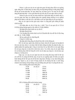
both simple and pure shear. To measure strain, fossils or
other objects of regular shape and size can be used. If the
original proportions and lengths of different parts in the
body of a particular species are known (Fig. 3.85a), it is
possible to determine linear strain for the rocks in which
they are contained. Figure 3.85 shows an example of
homogeneous deformation in trilobites (fossile arthropods)
deformed by simple shear (Fig. 3.85b) and pure shear
(Fig. 3.85c). Note how two originally perpendicular lines
in the specimen, in this case the cephalon (head) and the
bilateral symmetry axis of the body, can be used to meas-
ure the shear angle and to calculate shear strain.
88 Chapter 3
Fig. 3.83 Examples of measuring the angular shear in a square object
(a) deformed into a rectangle by pure shear (b) and a rhomboid (c)
by simple shear.
90°
90°
c
c
c
Angular shear γ
g = tan c
g = tan 30° = 0.57
g = tan c = tan –32° = –0.62
30°
–32°
(a)
(b)
(c)
a
a
b
bЈ
aЈ
(3)
LEED-Ch-03.qxd 11/27/05 4:26 Page 88
3.14.6 The strain ellipse and ellipsoid
We have seen earlier (Figs 3.80 and 3.84) that when homo-
geneous deformation occurs any circle is transformed into
a perfectly regular ellipse. This ellipse describes the change
in length for any direction in the object after strain; it is
called the strain ellipse. For instance, the major axis of the
ellipse, which is named S
1
(or e
1
), is the direction of maxi-
mum lengthening and so the circle is mostly enlarged in
this direction. Any other lines having different positions on
the strained objects which are parallel to the major axis of
the ellipse suffer the maximum stretch or extension.
Similarly the minor axis of the ellipse, which is known as S
3
(or e
3
) is the direction where the lines have been shortened
most, and so the values of the extension e and the stretch S
are minimum. The axis of the strain ellipse S
1
and S
3
are
known as the principal axis of the strain ellipse and are
mutually perpendicular. The strain ellipse records not only
the directions of maximum and minimum stretch or exten-
sion but also the magnitudes and proportions of both
parameters in any direction. To understand the values of
the axis of the strain ellipse imagine the homogeneous
deformation of a circle having a radius of magnitude 1,
which will be the value of l
0
(Fig. 3.86a). Now, if we apply
the simple equation of the stretch S (Equation 2; Fig. 3.81)
whereas for a given direction, the stretch e is the difference
in length between the radius of the ellipse and the initial
undeformed circle of radius 1 it is easy to see that the major
axis of the ellipse will have the value of S
1
and the minor
axis the value of S
3
. An important property of the strain
axes is that they are mutually perpendicular lines which
were also perpendicular before strain. Thus the directions
Forces and dynamics 89
y
y
y
x
x
x
c
Flattening direction
(a)
(c)
(b)
Fig. 3.84 Pure shear (a) and simple shear (b) are two examples of homogeneous strain. Both consist of distortions (no area or volume changes
are produced; (c) Simple shear has been classically compared to the shearing of a new card deck whose cards slide with respect to each other
when pushed (or sheared) by hand in one direction.
ψ
(a) (b) (c)
Fig. 3.85 Homogeneous deformation in fossil trilobites: (a) nondeformed specimen; (b) deformed by simple shear. Note how two originally
perpendicular lines such as the cephalon base and the bilateral symmetry axis can be used to measure the shear angle and calculate shear strain
(c) deformed by pure shear. If the original size and proportions of three species is known, linear strain can be established.
LEED-Ch-03.qxd 11/27/05 4:27 Page 89
of maximum and minimum extension or stretch corre-
spond to directions that do not experience (at that point)
shear strain (note the analogy with the stress ellipse in
which the principal stress axis are directions in which no
shear stress is produced). Shear strain can be determined in
the ellipse by two originally perpendicular lines, radii R of
the circle and the line tangent to a radius at the perimeter
(Fig. 3.87). In (a), before deformation, the tangent line to
the circle is perpendicular to the radius R. In (b), after
deformation, the lines are no longer normal to each other
and so an angular shear can be measured and the shear
strain calculated, as explained earlier.
In strain analysis two different kinds of ellipse can be
defined, (i) the instantaneous strain ellipse which defines
the homogeneous strain state of an object in a small incre-
ment of deformation and (ii) the finite strain ellipse which
represents the final deformation state or the sum of all the
phases and increments of instantaneous deformations that
the object has gone through. In 3D a regular ellipsoid will
develop with three principal axes of the strain ellipsoid,
namely S
1
, S
2
, and S
3
, being S
1
ՆS
2
ՆS
3
.
Now that we have introduced the concept of the strain
ellipse we can return to the previous examples of homoge-
neous deformation and have a look at the behavior of the
strain axes. In the example of Fig. 3.84 the familiar square
is depicted again showing an inner circle (Fig. 3.88). Two
mutually perpendicular radius of the circle have been
marked as decoration. Note that a pure shear strain has
been produced in four different steps. The circle
has become an ellipse that, as the radius of the circle has
a value of 1, will represent the strain ellipsoid, with two
principal axes S
1
and S
3
. Note that when a pure shear is
produced the orientation of the principal strain axis
remains the same through all steps in deformation and so
it is called coaxial strain (Fig. 3.88). This means that the
directions of maximum and minimum extension are pre-
served with successive stages of flattening. A very different
situation happens when simple shear occurs (Fig. 3.89):
the axes of the strain ellipsoid rotate in the shear direction
90 Chapter 3
Fig. 3.86 The stress ellipse in 2D strain analysis reflects the state of
strain of an object and represents the homogeneous deformation of
a circle of radius ϭ 1 transformed into an ellipsoid. As I
0
is 1,
S
1
ϭ I
1
/1 ϭ I
1
which represents the stretch S of the long axis.
Similarly S
3
ϭ I
1
giving the stretch S of the short axis.
S
3
S
3
r = 1
S
1
S
1
Before
deformation
Pure shear
Simple shear
(a)
(b)
(c)
Fig. 3.87 Shear strain in the strain ellipse. In (a), before deformation, the tangent line to the circle is perpendicular to the radius R. In (b), after
deformation, both lines are not normal to each other, the angular shear can be obtained and the shear strain calculated by tracing a normal line
to the tangent to the circle at the point where R’ intercepts the circle, and measuring the angle . The shear strain can be calculated as y ϭ tan .
R = 1
S
3
S
1
+c
R
R‘
(a) (b)
LEED-Ch-03.qxd 11/27/05 4:27 Page 90
After deformation, the circle has suffered strain and devel-
oped into a perfect ellipse by homogeneous flattening
(Fig. 3.90b). The original radius R of the circle, with
length l
0
, has been elongated and will correspond to the
radius RЈ of the ellipse of length l
1
. Comparing both
lengths, the extension, e (Equation 1; Fig. 3.81) or the
stretch, S (Equation 2; Fig. 3.81), can be easily calculated.
The reciprocal quadratic elongation can be directly
obtained as Јϭ(l
0
/l
1
)
2
. The angular deformation can be
measured by plotting the tangent to the ellipse at the point
p, where the radius intercepts the ellipse perimeter, then
plotting the normal to the tangent, and measuring the
angle with respect to the radius RЈ (Fig. 3.90b).
The Mohr circle strain diagram is a useful tool to graph-
ically represent and calculate strain parameters, following a
similar procedure that was used to calculate stress compo-
nents. In this case the ratio between the shear strain and the
quadratic elongation (␥/) is represented on the vertical
axis and the reciprocal quadratic elongation (Ј) on the
horizontal axis (Fig. 3.90c). The ␥/ ratio is an index of
the relative importance of the angular deformation versus
the linear elongation. When the ratio is very small, changes
in length dominate, in fact when the ratio equals zero,
there is no shear strain, which coincides with the directions
of the principal strain axis. In homogeneous strain of pure
Forces and dynamics 91
and so the strain is noncoaxial. The orientation of the axes
is not maintained, which means that the directions of max-
imum and minimum extension rotate progressively with
time.
3.14.7 The fundamental strain equations and
the Mohr circles for strain
For any strained body the shear strain and the stretch can
be calculated for any line forming an angle with respect
to the principal strain axis S
1
if the orientation and values
of S
1
and S
3
are known. As in the case of stress analysis
the approach can be taken in 2D or 3D. Although it is
important to remember that the physical meanings of
strain and stress are completely different, the equations
have the same mathematical form (Fig. 3.90) and can be
derived using a similar approach. The fundamental strain
equations allow the calculation of changes in length of
lines, defined by means of the reciprocal quadratic elonga-
tion(Јϭ1/), of any line forming an angle with
respect to the direction of maximum stretch S
1
. To illus-
trate the use and significance of the Mohr circles for strain,
an original circle of radius R can be used (as in Fig. 3.87).
Fig. 3.88 Pure shear is considered to be a coaxial strain since the orientation of the axes of the strain ellipse S
1
and S
3
remain with the same
orientation through progressively more deformed situations.
S
1
S
3
S
1
S
3
S
1
S
3
S
1
S
3
r = 1
Fig. 3.89 Simple shear can be described as a noncoaxial strain as the orientation of the principal strain axis of the strain ellipse S
1
and S
3
rotates
with progressive steps on deformation.
S
1
S
3
S
3
S
1
S
3
S
1
S
3
S
1
r = 1
LEED-Ch-03.qxd 11/27/05 4:27 Page 91
distortion, where there is no change in volume or area,
there are two directions that suffer no finite stretch, where
the value of ϭ 1. Finally two directions of maximum shear
strain are present, corresponding to the lines forming an
angle ϭ 45Њ with respect to S
1
. The Mohr circle for strain
has an obvious relation to the fundamental strain equations
(Equations 4 and 5; Fig. 3.90a) as shown in Fig. 3.90d.
To plot the circle in the coordinate axes, the reciprocal
values Ј
1
and Ј
3
of
1
and
3
are first calculated and rep-
resented along the horizontal axis. The circle will have a
diameter Ј
3
Ϫ Ј
1
and the center will have coordinates
(Ј
1
ϩ Ј
3
)/2, 0. Note that as the expressions on the x-axis
are the reciprocal quadratic elongations, the maximum
value, at the right end of the circle, corresponds to Ј
3
and
the minimum, at the left end, to Ј
1
. Once the circle is
plotted, it is possible to calculate the values of ␥/ and Ј
(Fig. 3.90d) for any line forming an angle respect to the
direction of the major principal strain axis S
1
. The line is
plotted from the center of the circle at the angle 2 sub-
tended from Ј
1
into the upper half of the circle if the
angle is positive or into the lower half if it is negative. The
coordinates of the point of intersection between the line and
the circle have the values ␥/, Ј. Through Ј the value of
and then that of S can be calculated. Knowing it is
also possible to calculate ␥ and finally the angle of shear
strain .
92 Chapter 3
Fig. 3.90 (a) The fundamental strain equations. The Mohr circles for strain display graphically the relations between the ␥/ ratio and the
reciprocal quadratic elongation Ј. The ␥/ ratio reflects the relative importance of angular deformation versus linear deformation; (b) strained
circle into an ellipse; (c) the Mohr circle strain diagram; and (d) Relation between the Mohr circle and the fundamental strain equations.
The fundamental strain equations
Considering the quadratic elongation l = (1 + e)
2
= S
2
(1)
l =
l
1
+ l
3
+
l
1
– l
3
cos 2f
22
l‘ =
lЈ
1
+ lЈ
3
–
lЈ
3
– lЈ
1
cos 2f
22
g /l =
lЈ
3
– lЈ
1
sin 2f
2
To define the strain equations, the reverse of the quadratic
elongation, or reciprocal quadratic elongation (l’) is used:
lЈ = 1/l
g/l
g/l
lЈ
lЈ
1
lЈ
lЈ
3
g/l
lЈ
lЈ
lЈ
1
lЈ
3
2
lЈ
3
–
lЈ
1
2
lЈ
3
–
lЈ
1
sin 2
u
2
2f
2f
lЈ
3
–
lЈ
1
cos 2
f
2
l
3
l
1
g =tan c
f
(b)
(d)
(c)(a)
+ c
RЈ
Equation 5 relates the ratio between the angular
strain g and the linear strain l, with the principal strain axis
and the angle f.
p
lЈ
1
+ lЈ
3
(2)
(3)
(4)
(5)
3.15 Rheology
3.15.1 Rheological models
The reaction of rock bodies and other materials to applied
stresses can only be observed and studied through laboratory
experiments: the study of strain–stress relations or how the
rocks or other materials respond to stress under certain con-
ditions is the concern of rheology. Different kinds of experi-
ments are possible, generally undertaken on centimeter-scale
LEED-Ch-03.qxd 11/27/05 4:27 Page 92
cylindrical rock samples. Both tensional (the sample is gen-
erally pulled along the long axis) and compressive (sample
is pushed down the long axis) stresses can be applied, both
in laterally confined (axial or triaxial tests) or unconfined
conditions (uniaxial texts). Experiments involving the
application of a constant load to a rock sample and observ-
ing changes in strain with time are called creep tests.
Experimental results are analyzed graphically by plotting
stress, (), against strain, (), or strain rate (d/dt), the
latter obtained by dividing the strain by time (Fig. 3.91).
Simple mathematical models can be developed for different
regimes of rheological behavior. Stress is usually repre-
sented as the differential stress (
1
Ϫ
3
). Other important
variables are lithology, temperature, confining pressure,
and the presence of fluids in the interstitial pores
causing pore fluid pressures. There are three different pure
rheological behavioral regimes: elastic, plastic, and viscous
(Fig. 3.91). Elastic and plastic are characteristic of solids
whereas viscous behavior is characteristic of fluids. Solids
under certain conditions, for example, under the effect of
permanent stresses, can behave in a viscous way. Elastic,
plastic, and viscous are end members of a more complex
suite of behaviors. Several combinations are possible, such
as visco-elastic, elastic–plastic, and so on.
3.15.2 Elastic model
Elastic deformation is characterized by a linear relationship
in stress–strain space. This means that the relation between
the applied stress and the strain produced is proportional
(Fig. 3.91a). An instantaneous applied stress is followed
instantly by a certain level of strain. The larger the stress
the larger the strain, up to a point at which the rock can be
distorted no further and it breaks. This limit is called the
elastic boundary and represents the maximum stress that
the rock can suffer before fracturing. If the stress is
released before reaching the elastic limit such that no frac-
tures are produced, elastic deformation disappears. In
other words, elastic strained bodies recover their original
shape when forces are no longer applied. The classical ana-
log model is a spring (Fig. 3.92a). The spring at repose
represents the nondeformed elastic object. When a load is
Forces and dynamics 93
Fig. 3.91 Strain/stress diagrams for different rheological behaviors.
(a) Elastic solids show linear relations. The slope of the straight line
is the Young’s modulus; (b) viscous behavior is characteristic of flu-
ids. Fluids deform continuously at a constant rate for a certain stress
value. The slope of the line is the viscosity (); (c) plastics will not
deform under a critical stress value or yield stress (
y
).
Strain (e)
Stress (s)
Elastic
(a)
(c)
(b)
E= s/e
Strain rate de/dt
Stress (t)
Viscous
h = t
de/dt
Strain (e)
Stress (s)
Plastic
s
y
Fig. 3.92 Classical analogical models for (a) elastic behavior, is
compared to a spring; (b) viscous behavior is compared to a
hydraulic piston or dashpots; and (c) plastic behavior, like moving
a load by a flat surface with an initial resistance to slide.
(a)
(b)
(c)
s
>
s
y
s
<
s
y
Object is static
Object moves
Heavy
Heavy
LEED-Ch-03.qxd 11/27/05 4:27 Page 93
added to the spring in one of the extremes (as a
dynamometer) or it is pulled by one of the edges, it will
stretch by the action of the applied force. The bigger the
load, or the more the spring is pulled on the extremes, the
longer it becomes by stretching. When the spring is
released or liberated from the load in one of the extremes
the spring returns to the original length.
Elasticity in rocks is defined by several parameters; the
most commonly used being Young’s modulus (E) and
the Poisson coefficient (). Young’s modulus is a measure of
the resistance to elastic deformation which is reflected in the
linear relation between the stress () and the strain (): E ϭ
/ (Fig. 3.93a). This linear relation, which was observed
initially by Hooke in the mid-seventeenth century by apply-
ing tensile stresses to a rod and measuring the extension, is
commonly known as Hooke’s Law. Considering that all
parameters used to measure strain (stretch, extension, or
quadratic elongation) are dimensionless, the Young’s modu-
lus is measured in stress units (N m
Ϫ2
, MPa) and has negative
values of the order of Ϫ10
4
or Ϫ10
5
. The reason why the
values are negative is because the applied stress is extensional
and hence has a negative value, and the strain produced is a
lengthening, which is conventionally considered positive.
Not all rocks follow Hooke’s Law; some deviations occur
but they are small enough so a characteristic value of E can
be defined for most rock types (Fig. 3.93a). A high absolute
value for the Young’s modulus means that the level of strain
produced is small for the amount of stress applied, whereas
low values indicate higher deformation levels for a certain
amount of stress. Rigid solids produce high Young’s modu-
lus values as they are very reluctant to change shape or vol-
ume. Rigid materials experience brittle deformation when
their mechanical resistance is exceeded by the applied stress
level at the elastic boundary.
When applying uniaxial compressional tests to rock
samples, vertical shortening may be accompanied by some
horizontal expansion. The Poisson coefficient () shows
the relation between the lateral dilation or barreling of a
rock sample and the longitudinal shortening produced by
loading: thus ϭ
lateral
/
longitudinal
and it can be seen that
Poisson’s coefficient is dimensionless (Fig. 3.93b). When
stresses are applied, if there is no volume loss, the sample
has to thicken sideways to account for the vertical shorten-
ing. Typically, the sample should develop a barrel form
(nonhomogeneous deformation) or increase its surface
area as it expands laterally. For perfect, incompressible,
isotropic, and homogeneous materials which compensate
the shortening by lateral dilation without volume loss, the
Poisson’s coefficient is 0.5; although values for natural
materials are generally smaller (Fig. 3.93b). In very rigid
rock bodies, the lateral expansion may be very limited
or not occur at all; in this case there is a volume loss and
94 Chapter 3
e (%)
s
1
− s
3
(MPa)
a
b
E = s/e (Hooke’s Law)
(a)
(b)
E
a
> E
b
Marble
Limestone
Granite
Shale
Quartzite
Diorite
–4.8
–5.3
–5.6
–6.8
–7.9
–8.4
Rock type E (ϫ10
4
MPa)
Schist, biotite
Shale, calcareous
Diorite
Granite
Aplite
Siltstone
Dolerite
0.01
0.02
0.05
0.11
0.20
0.25
0.28
Rock type n
Final state
Original
Uniaxial
compression
n = ed/ec
c
d
ec
ed
Fig. 3.93 Elastic parameters. (a) The Young’s modulus describes the slope of the stress/strain straight line, being a measure of the rock
resistance to elastic deformation. Line a has a higher value of Young’s modulus (E
a
) being more rigid than line b (Young modulus E
b
)
(i.e. it is less strained for the same stress values); (b) Poisson’s coefficient relates the proportion in which the rock deforms laterally when it is
compressed vertically. Comparing the original and final lengths before and after deformation strain can be calculated and the Poisson’s ratio
established.
LEED-Ch-03.qxd 11/27/05 4:27 Page 94
elastic stresses have to be accumulated somehow. Rock
samples will fragment at the elastic limit after experiencing
very little lateral strain when the Poisson’s ratio is very
small (close to zero). The reciprocal to the Poisson’s coef-
ficient is called the Poisson’s number m ϭ 1/. This num-
ber is also constant for any material, and so the relation
between the longitudinal and lateral strains have a linear
relation. Nonetheless, as in the case of Young’s modulus
there may be slight variations in the linear trend of
Poisson’s coefficient (Fig. 3.94). It is important to remem-
ber that experiments to establish elasticity relationships
under unconfined uniaxial stress conditions allow the rock
samples to expand laterally. In the crust, any cube of rock
that we can define is not only subject to a vertical load due
to gravity but also due to adjacent cubes of rock in every
direction and is not free to expand laterally; in such cases
complex stress/strain relations can develop.
Other elastic parameters are the rigidity modulus (G)
and the bulk modulus (K). The rigidity modulus or shear
modulus is the ratio between the shear stress () and the
shear strain (␥) in a cube of isotropic material subjected to
simple shear: G ϭ /␥ (Fig. 3.95). G is another measure of
the resistance to deformation by shear stress, in a way
equivalent to the viscosity in fluids. The bulk modulus (K)
relates the change in hydrostatic pressure (P) in a block of
isotropic material and the change in volume (V) that it
experiences consequently: K ϭ dP/dV. The reverse to the
bulk modulus is the compressibility (1/K).
3.15.3 Viscous model
Viscous deformation occurs in fluids (Sections 3.9 and 3.10);
fluids have no shear strength and will flow when shear
stresses, even infinitesimal, are applied. One of the chief
differences between an elastic solid and a viscous fluid is
that when a shear stress is applied to a piece of elastic mate-
rial it causes an increment of strain proportional to the
stress, if the same level of stress is maintained no further
deformation is achieved (Fig. 3.96a). In fluids when a
shear stress () is applied the material suffers certain
amount of strain but the fluid keeps deforming with time
even when the stress is maintained with the same value
(Fig. 3.96b). In this case a level of stress gives way to a
strain rate (d/dt), not a simple increment of strain as in
the elastic solids. Higher stress values will give way to
higher strain rates, so the fluid will deform at more speed.
As in elastic materials there is no initial resistance to
deformation even when stresses acting are very small, but
the deformations are permanent in the viscous fluid case
(Fig. 3.97a,b).
As we have seen earlier (Sections 3.9 and 3.10) the parame-
ter relating stress to strain rate is the coefficient of dynamic vis-
cosity or simply viscosity (): ϭ /(d/dt), which is
Forces and dynamics 95
Fig. 3.94 Longitudinal and lateral strain experienced by a rock
sample when an uniaxial compression is applied. The relation
between both strains may not be linear as in this case, and the
Poisson’s ratio is not constant, it varies slightly for different stress
values.
ShorteningDilation
Longitudinal
strain
Lateral
strain
e
s
E=s/e
Fig. 3.96 (a) Solid elastic bodies are strained proportionally to the
applied forces. If the intensity of the force is maintained there is not a
further increase in strain. When the force is released the object
recovers the initial shape; (b) The viscous fluid will be deformed
when a shear force is exerted, but even when the intensity of the
force is maintained, an increment in deformation will occur, defining
a strain rate. That is why strain rate is used in rheological plots
instead of strain as in solids. The fluid body will remain deformed
permanently once the force is removed.
Solid elastic body
Fluid viscous body
(a)
(b)
Fig. 3.95 Shear or rigidity modulus (G) and its relation to Young’s
modulus (E) and Poisson’s number (m).
t
c
g = tan
c
G = t/g
G =
2m + 1
mE
LEED-Ch-03.qxd 11/28/05 10:01 Page 95
measured in Pascals. Fluids that show a linear relation between
the stress and the strain rate, and so have a constant viscosity,
are called Newtonian. Fluids, whose viscosity changes with the
level of stress are called non-Newtonian (Fig. 3.98). Viscous
behavior is generally compared to a piston or a dashpot con-
taining some hydraulic fluid (Fig. 3.92b). The fluid is pressed
by the piston (creating a stress or loading) and the fluid moves
up and down a cylinder, producing permanent deformation;
the quicker the piston moves the more rapid the fluid deforms
or flows up and down. The viscosity can be described as the
resistance of the fluid to movement. High viscosity fluids are
more difficult to displace by the piston up and down the cylin-
der. For non-Newtonian fluids (Fig. 3.98) as the piston is
pushed more and more strongly in equal increments of added
stress the rate of movement or strain rate rapidly increases in a
non-linear fashion.
3.15.4 Plastic model
Plastic deformation is characteristic of materials which do
not deform immediately when a stress is applied. A certain
96 Chapter 3
Fig. 3.97 Strain of different materials with time (stages T1 to T5)
applying increasing levels of stress: (a) Elastic solids show discrete
strain increments with increasing stress levels (linear relation);
strain is reversible once the stress is removed (T 5); (b) Viscous
fluids flow faster (higher strain rates) with increasing stress; the
deformation is permanent once the stress is released; (c) Plastic
solids will not deform until a critical threshold or yield stress is
overpassed (at T4 in this case). Deformation is nonreversible
(at T5).
TIME
s < s
y
s > s
y
T1
T2 T3
T4 T5
(a) Elastic
(c) Plastic
(b) Viscous
Stress released
Final state
Increassing stress applied
level of stress is required to start deformation, as the mate-
rial has an initial resistance to deformation. This stress
value is called yield stress
y
(Fig. 3.91c). After the yield
stress is reached the body of material will be deformed a
big deal instantaneously, and the deformation will be per-
manent and without a loss of internal coherence. So, two
important differences with respect to elastic behavior are
that the strain is not directly proportional to the stress, as
there is an initial resistance, and that the strain is not
reversible as in elastic behavior (Fig. 3.97). An analogical
model for plastic deformation is that of a heavy load rest-
ing on the floor (Fig. 3.92c). If the force used to slide the
load along a surface is not big enough, the load will not
budge. This would depend on the frictional resistance
exerted by the surface. Once the frictional resistance, and
so the yield stress, is exceeded, the load will slide easily and
the movement can be maintained indefinitely as long as
the force is sustained at the same level over the critical
threshold or yield stress. The load will not go back on its
own! So the deformation is not reversible (Fig. 3.92c).
3.15.5 Combined rheological models
Elastic, viscous, and plastic models correspond to simple
mathematical relationships which apply to materials under
Fig. 3.98 Viscosity is the resistance of a fluid to deform or flow: it is
the slope of the curve stress/strain rate. Fluids showing linear
relations (constant viscosity) are Newtonian. Fluids with nonlinear
relation ( variable) are non-Newtonian. The table shows the values
of viscosity () for some viscous materials.
Strain rate de/dt
Stress (t)
h =
t
de/dt
Newtonian
non-Newtonian
Water (30º)
Oil
Basalt lava
Rhyolite lava
Salt
Asthenosphere
0.8 и 10
–3
0.08
10
2
10
8
10
16
10
22
Fluid h (Pa)
(h constant)
(h variable)
LEED-Ch-03.qxd 11/27/05 4:29 Page 96
ideal conditions; they are considered homogeneous (the
rock has the same composition in all its volume) and
isotropic (the rock has the same physical properties in all
directions). Rocks are rarely completely homogeneous or
isotropic due to their granular/crystalline nature and
because of the presence of defects and irregularities in the
crystalline structure, as well as layers, foliations, fractures,
and so on. Nevertheless, although such aberrations would
be important in small samples, on a large scale, when large
volumes are being considered, rocks can be sometimes
regarded as homogeneous. Usually, however, natural rhe-
ological behavior corresponds to a combination of two or
even three different simple models, such as elastic–plastic,
visco-elastic, visco-plastic, or elastic–visco-plastic. Also
materials can respond to stress differently depending on
the time of application (as in instantaneous loads versus
long-term loads).
A well-known example of a combined rheological model
is the elastic–plastic (Prandtl material) (Fig. 3.99); it shows
an initial elastic field of behavior where the strain is recov-
erable, but once a yield stress (
y
) value is reached the
material behaves in a plastic way. The analogical model is a
spring (elastic) attached to a heavy load (plastic) moving
over a rough surface (Fig. 3.99b). The spring will deform
instantly whereas the load remains in place until the yield
stress is reached, then the load will move; after releasing
the force, the spring will recover the original shape but the
longitudinal translation is not recoverable. Elastic–plastic
materials thus recover part of the strain (initial elastic) but
partly remain under permanent strain (plastic). Remember
that in a pure elastic material, permanent strain does not
occur and after the elastic limit is reached the rock breaks
(b, Fig. 3.99c; line I) whereas in a Prandtl material there is
a nonreversible strain (c, Fig. 3.99c, line II). Once the plastic
limit is reached, the material can then break but only after
suffering some permanent barreling (d, Fig. 3.99c, line II).
Visco-elastic models correspond to solids (called
Maxwell materials) which have no initial resistance to
Forces and dynamics 97
Fig. 3.99 (a) Elastic–plastic material shows an initial elastic field characterized by recoverable deformation strain followed by a plastic field in
which the strain is permanent. The boundary between both fields is the elastic limit located at the yield stress value (
y
); (b) The analog model
is a load attached to a spring; (c) Part of the strain is recovered (the length of the spring) and part is not (the displacement of the load).
b. elastic limit
elastic limit
Stress (s
1
–s
3
) MPa
strain (ε)
d. plastic limit
time
a
b
c
c
d
strain (e)
stress (s)
Elastic – Plastic
elastic
limit
elastic field
plastic field
s
y
s
y
(b)
(a)
(c)
I
II
a
a
Prandtl material
F
LEED-Ch-03.qxd 11/27/05 4:30 Page 97
strain as in both elastic and viscous models (Fig. 3.100a).
Part of the strain will recover following an elastic behavior
but part will remain permanently deformed. Maxwell
solids behave elastically when the stresses are short lived,
like a ball of silicon putty that bounces elastically on the
floor when thrown with some force; but will accumulate
permanent deformations at a constant rate if the stress or
load (like the proper weight of the material) is applied for
a longer time. Visco-elastic models can be represented by
a spring attached longitudinally to a dashpot (Fig. 3.100b).
The spring will provide the recoverable strain whereas the
dashpot will supply the nonrecoverable strain when a
pulling force is applied parallel to the system.
Visco-plastic materials (called Bingham plastics) only
behave like viscous fluids after reaching a yield stress, the
strain rate subsequently being proportional to the stress;
initially the material does not respond to the applied stress
as for plastic solids (Fig. 3.100c). The analogy will be in
this case a dashpot attached in parallel to a load sliding on
a surface with an initial resistance to movement; once the
load is in motion it behaves in viscous fashion.
3.15.6 Ductile and brittle deformation
From the different rheological models discussed above it
can be concluded that there are several kinds of deforma-
tion. First, strain produced when loads are applied can be
reversible; this is characteristic of elastic behavior as in the
elastic curves or elastic–plastic materials (a, Fig. 3.99c)
when small stress increments are applied. Deformations can
also be nonreversible, which means that once the load is
released the rock will be deformed permanently.
Deformation is said to be ductile when rocks or other solids
are strained permanently without fracturing, which hap-
pens in plastic or elastic–plastic materials once the elastic
limit or yield strength (stress value which separates the elas-
tic and plastic fields) is reached (as c in Fig. 3.99c).
98 Chapter 3
Fig. 3.100 (a) Visco-elastic or Maxwell materials have a recoverable strain part belonging to the elastic component and a permanent strain
due to the viscous behavior like a spring attached to a dashpot (b); (c) visco-plastic or Bingham materials behave in a viscous way but after
reaching a critical stress value or yield stress (
y
) like a dashpot linked to a load moving on a rough surface (d).
s
y
Stress (s)
(a)
(b)
(c) (d)
Stress (s)
Strain rate d/dt
Strain rate de/dt
Maxwell material
Bingham material
F
F
LEED-Ch-03.qxd 11/27/05 4:30 Page 98
Nonetheless, ductile is a general, descriptive term that does
not involve a specific rheological behavior or strain mecha-
nism. It is not a synonymous term for plastic, which is a very
well-defined and particular rheological behavior. Strains pro-
duced during plastic deformations are larger in magnitude
than those produced in the elastic field and are generally
formed by dislocations of the crystalline lattices and/or dif-
fusive processes. Ductile deformations are also called ductile
flows as the material deforms or flows in a solid state (as a gla-
cier sliding downslope does, Section 6.7.5). Examples of
ductile deformation in rocks are the formation of folds and
salt diapirs. Rocks have a limited ability to change their shape
or volume, which also depends on such external parameters
as the temperature, confining pressure, and so on.
Brittle deformation happens when the internal strength
of rocks is exceeded by stresses; they bust, so internal
cohesion is lost in well-defined surfaces or fractures. Brittle
deformation can occur after the elastic limit is exceeded
not only in pure elastic bodies (b, Fig. 3.99c) but also
when the stresses reach the plastic limit after some ductile
deformation has taken place. Such samples will be perma-
nently deformed and also fractured (d, Fig. 3.99c).
3.15.7 Parameters controlling rock deformation
Lithology (rock type) is a variable which may cause diverse
modes of stress–strain behavior. Different rocks or sub-
stances may need different rheological models with which
to describe their deformation. Competency is a qualitative
term used to describe rocks in terms of their inner strength
or capacity for deformation. Rocks which deform easily
and generally in a ductile way are described as incompetent,
such as salts, shale, mudstone, or marble. Strong or compe-
tent rocks are those which are more difficult to deform,
such as quartzite, granite, quartz sandstones, or fresh
basalts. Competent rocks are stiffer and deform generally
in a brittle way. Nevertheless, competency depends not
only on lithology but also on temperature, confining pres-
sure, pore pressure, strain rate, time of application of the
stress, etc. To compare competencies of different kinds of
rocks, experiments must take place at equal temperatures
and confining pressures.
Temperature has particularly important effects in rheo-
logical behavior (Fig. 3.101). Comparing several experi-
ments on samples of the same lithology under the same
conditions of confining pressure, it is possible to compare
stress–strain relations at different temperatures. At higher
temperatures, rocks behave in a more ductile way, so com-
petence is reduced and fractures are more difficult to pro-
duce. For rocks that are elastic at low temperatures a
plastic field can develop. In elastic–plastic materials, tem-
perature lowers the elastic limit, which is thus reached at
lower stress levels. Rocks may also behave in a viscous way
at high temperatures if the applied stresses are long lasting.
Confining pressure (lithostatic or hydrostatic pressure
acting on all sides of a rock volume) can be simulated in
laboratory experiments by introducing some fluid that
exerts a certain amount of pressure in the sample (triaxial
tests) in addition to that provided by the compressive load,
and by isolating the sample in a constraining metal jacket
to discriminate and separate the effects of the pore pres-
sure in the rock. Experiments carried out on samples of the
same lithology and at the same temperature show that
higher confining pressures increase the yield strength in a
rock, and also the plastic field, so fracturing, if it happens,
occurs after more intense straining (Fig. 3.102). This
means that rocks became more ductile at higher levels of
confining pressure.
When there is fluid trapped in the rock pores, it exerts an
additional hydrostatic pressure which has the effect of
counteracting the confining pressure by the same value of
the fluid pressure in the pores. The state of stress is lowered
and an effective stress tensor can be defined by subtracting
the values of the fluid stresses from those of the solid
normal stresses (Fig. 3.103). The Mohr circle moves
toward lower values by an amount equal to the pore pressure
(p
f
) sustained by the fluid. Thus, when fluids are present in
the pores the effect is the same as lowering the confining
Forces and dynamics 99
Fig. 3.101 Effect of temperature in the strain–stress diagram for
basalts under the same confining pressure (5 kbars).
2.0
1.5
1.0
0.5
0
Differential stress (×10
3
MPa)
Strain, e (%)
0 5 10 15
25°C
300°C
500°C
800°C
700°C
LEED-Ch-03.qxd 11/27/05 4:30 Page 99
pressure in the rocks, so that ductility decreases and frac-
tures are produced more easily. Being hydrostatic in nature,
the effectiveness of the normal stresses is lowered but the
shear stresses remain unaltered. The control of pore pres-
sure in the rocks is of key importance in fracture formation
and will be discussed in some more detail in Section 4.14.
Other important factors are the time of application of the
stresses: the instantaneous or long-term application of a
certain level of stress may cause different rheological behav-
iors, like the case of the silicon putty discussed earlier. Rock
strength decreases when the stresses are applied for long
times under small differential stresses (creep experiments).
Also in relation to time, the rates of loading (velocity of
increased loading in the experiments) also have important
implications for the production of strain. In a single exper-
iment, the rate of strain is generally maintained constant
but the rates of strain can be changed from one experiment
to another. When changes in strain are produced rapidly
(high loading rates) the rock samples become ductile and
break at higher stress levels.
100 Chapter 3
Fig. 3.102 (a) Strain–stress diagram showing several curves corresponding to limestone samples of the same composition at different confining
pressures (in MPa); (b) Differences in confining pressure give way to different fracturing or deformation modes. Confining pressure from samples
(from 0.1 to 35 MPa in the fractured samples and 100 MPa for the ductile flow).
Differential stress (MPa)
Strain, e (%)
20
40
60
70
80
130
140
300
200
100
0
0 2 4 6 8 10 12 14 16
Limestone
(a) (b)
12
43
Fig. 3.103 When there is some pressurized fluid in the rock pores, part of the stress is absorbed. The state of stress is lowered and an effective stress
tensor can be defined subtracting the values of the normal stresses from those of the fluid. The Mohr circle moves toward lower values by an
amount equal to the pore pressure (P
f
) sustained by the fluid.
t
s
n
E
s
1
E
s
3
Applied stressEffective stress
0
s
1
s
2
E
s
2
s
3
Pore fluid pressure
(P
f
)
s
pf
0 0
0 s
pf
0
0 0
σ
pf
s
xx
t
xy
t
xz
t
yx
s
yy
t
yx
t
zx
t
zy
s
zz
−
Es =
s
xx
–s
pf
t
xy
t
xz
t
yx
s
yy
-s
pf
τ
yx
t
zx
t
zy
s
zz
–s
pf
Es =
Hydrostatic stress
(fluid)
Applied stress
(rock)
LEED-Ch-03.qxd 11/27/05 4:30 Page 100
P.M. Fishbane et al.’s Physics for Scientists and Engineers:
Extended Version (Prentice-Hall, 1993) is again invaluable.
Many good things of oceanographic interest can be found
in the exceptionally clear work of S. Pond and G.L. Pickard
– Introductory Dynamical Oceanography (Pergamon,
1983), while R. McIlveen’s Fundamentals of Weather and
Climate (Stanley Thornes, 1998) is good on the atmos-
pheric side. A more advanced text is D.J. Furbish’s Fluid
Physics in Geology (Oxford, 1997). G.V. Middeton and P.R.
Wilcox’s Mechanics in the Earth and Environmental Sciences
has a broad appeal at intermediate level and is very thor-
ough. The best introduction to solid stress and strain is in
G.H. Davies and S.J. Reynolds’s Structural Geology of Rocks
and Regions (Wiley, 1996); R.J. Twise and E.M. Moores’s
Structural Geology (1992) and J.G. Ramsay and M. Huber’s
The Techniques of Modern Structural Geology, vol. 1: Strain
Analysis (Academic Press, 1993) are classics on structural
geology for advanced studies on solid stress. W.D. Means’s
Stress and Strain (Springer-Verlag, 1976) takes a careful and
rigorous course through the basics of the subject.
Forces and dynamics 101
Further reading
LEED-Ch-03.qxd 11/27/05 4:30 Page 101
Earth is a busy planet: what are the origins of all this
motion? Generally, we know the answer from Newton’s
First Law that objects will move uniformly or remain sta-
tionary unless some external force is applied. The uniform
motion of fluids must therefore involve a balance of forces in
whatever fluid we are dealing with. In order to try to predict
the magnitude of the motion we must solve the equations of
motion that we discussed previously (Section 3.12). Bulk
flow (in the continuum sense, ignoring random molecular
movement) involves motion of discrete fluid masses from
place to place; the masses must therefore transport energy:
mechanical energy as fluid momentum and thermal energy
as fluid heat. There will also be energy transfers between the
two processes, via the principle of the mechanical equivalent
of heat energy and the First Law of Thermodynamics
(Section 2.2, conservation of energy). For the moment we
shall ignore the transport of heat energy (see
Sections 4.18–4.20) since radiation and conduction intro-
duce the very molecular-scale motions that we wish to
ignore for initial simplicity and generality of approach.
4.1.1 Very general questions
1 How does fluid flow originate on, above, and within the
Earth? For example, atmospheric winds and ocean currents
originate somewhere and flow from place to place for certain
reasons. This raises the question of “start-up,” or the begin-
nings of action and reaction.
2 If fluid flow occurs from place A to place B, what hap-
pens to the fluid that was previously at place A? For exam-
ple, the arrival of an air mass must displace the air mass
previously present. This introduces the concept of an
ambient medium within which all flows must occur.
3 How does moving fluid interact with stationary or mov-
ing ambient fluid? For example, does the flow mix at all
with the ambient medium? If so, at what rate? How does
the interaction look physically?
4 What is the origin and role of variation in flow velocity
with time (unsteadiness problem)? It is to be expected that
accelerations will be very much greater in the atmosphere
than in the oceans and of negligible account in the solid
earth (discounting volcanic eruptions and earthquakes).
Why is this?
4.1.2 Horizontal pressure gradients and flow
Static pressure at a point in a fluid is equal in all directions
(Section 3.5) and equals the local pressure due to the
weight of fluid above. Notwithstanding the universal truth
of Pascal’s law, we saw in Section 3.5.3 that horizontal
gradients in fluid pressure occur in both water and air.
These cause flow at all scales when a suitable gradient
exists. The simplest case to consider is flow from a fluid
reservoir from orifices at different levels (Fig. 4.1). Here
the flow occurs across the increasingly large pressure gra-
dient with depth between hydrostatic reservoir pressure
and the adjacent atmosphere.
The gradient of pressure in moving water (Fig. 4.1) is
termed the hydraulic gradient, and the flow of subsurface
water leads to the principle of artesian flow and the basis of
our understanding of groundwater flow through the oper-
ation of Darcy’s law (developed from the Bernoulli
approach in Sections 4.13 and 6.7). The flow of a liquid
down a sloping surface channel is also down the hydraulic
gradient.
Similar principles inform our understanding of the slow
flow of water through the upper part of the Earth’s crust.
Here, pressures may also be hydrostatic, despite the fluid
held in rock being present in void space between solid rock
particles and crystals (Fig. 4.2); this occurs when the rocks
4 Flow, deformation,
and transport
4.1 The origin of large-scale fluid flow
Geostatic
gradient
Hydrostatic
gradient
Calculated
for:
r
water
= 1,000 kg m
–3
r
rock
= 2,380 kg m
–3
LEED-Ch-04.qxd 11/26/05 13:11 Page 102
Flow, deformation, and transport 103
u
2
u
1
u
3
h
1
h
2
h
3
p
0
= Atmospheric
h
0
Slope of line gives
hydraulic gradient
During flow from a reservoir along a
pipe or channel there is energy loss
downstream due to friction (drag)
Flow out
Exit velocity = u = √
2gh
Flow in
Escape from a reservoir at a rate
determined by the local difference
in pressure between hydrostatic and
atmospheric
Fig. 4.1 Flows induced by hydrostatic pressure.
In the hydrostatic condition
all liquid levels are equal
p
0
= Atmospheric
p
0
= Atmospheric
There is no change to this
principle when the fluid
occupies void space that
has continuous connection
to the surface
Fig. 4.2 The hydrostatic condition is equally valid for liquid in reser-
voirs or porous rock.
Pressure, kg m
–2
100
.
10
5
500
.
10
5
Depth km
1
2
3
Geostatic
gradient
Hydrostatic
gradient
Calculated for:
r
water
= 1,000 kg m
–3
r
rock
= 2,380 kg m
–3
Fig. 4.3 Hydrostatic and geostatic pressure gradients in the
Earth’s crust.
Strong wind causing wind shear
A
B
b
High
atmospheric
pressure
Low
atmospheric
pressure
and water “set-up” on lee-shore
Sloping isobars
High
Low
Subsurface flow down horizontal
hydrostatic pressure gradient
(modified by Coriolis force in 3D)
Fig. 4.4 Barotropic flow due to a horizontal gradient in hydrostatic pressure caused and maintained by atmospheric dynamics. The spatial
gradients in atmospheric pressure and wind shear may act together or separately. In both cases hydrostatic pressures above B are greater than
hydrostatic pressures at all equivalent heights above A, by a constant gradient given by the water surface slope.
are porous to the extent that all adjacent pores communi-
cate, as is commonly the case in sands or gravels. Severe
lateral and vertical gradients arise when pores are closed by
compaction, as in clayey rock; the hydrostatic condition
now changes to the geostatic condition when pore pres-
sures are greater due to the increased weight of overlying
rock compared to a column of pore water (Fig. 4.3).
Interlayering of porous and nonporous rock then leads to
high local pressure gradients down which subsurface fluids
may move. In passage down an oil or gas exploration well,
pressure may jump quickly from a hydrostatic trend toward
LEED-Ch-04.qxd 11/26/05 13:15 Page 103
104 Chapter 4
lithostatic, causing potentially disastrous consequences for
the drill rig and possible “blowout.” The regional
hydraulic gradient drives the direction of migration of
subsurface fluids like water and hydrocarbon. Pressures in
partially molten rocks of the Earth’s upper crust in crustal
magma chambers (Section 5.1) may also vary between
hydrostatic and geostatic values, with obvious implications
for the forces occurring during volcanic eruptions.
Ambient fluid
r
1
lockbox
fluid r
2
Conditions r
1
= r
2
Ambient liquid
r
1
Ambient liquid
r
1
Ambient gas
r
1
Ambient gas
r
1
lockbox
liquid ρ
2
Conditions r
1
< r
2
∆
r
= +ve
lockbox
liquid r
2
Conditions r
1
> r
2
∆
r
= –ve
lockbox
liquid r
2
Conditions r
1
< r
2
∆
r
= +ve
lockbox
liquid r
2
Conditions r
1
> r
2
∆
r
= –ve
Water surface
Water surface
Neutral stability for all cases
Surface jet
Rising plume
Rising plume (thermal)
Descending plume (open ocean
cold convection, ice meltout)
Wall jet
descending flow
(bottom water production,
turbidity currents)
Catabatic wind
Thunderstorm
downdraught
Sea breeze front
Cold front
Wall jet
(turbidity flow,
thermohaline flow)
Ocean and lakes (unstratified)
Atmosphere (unstratified)
open
open
open
open
open
Sloping boundary
Lower horizontal boundary
Ocean ridge
hydrothermal
plumes
Mixing by molecular diffusion only
Fig. 4.5 Buoyancy-driven flows.
LEED-Ch-04.qxd 11/26/05 13:16 Page 104
Flow, deformation, and transport 105
4.1.3 Flow in the atmosphere and oceans
The atmosphere and oceans are in a constant state of flux,
both experiencing “weather”; that is, the velocity of the
ocean waters and atmosphere is unsteady with respect to
either magnitude or direction over timescales of minutes
to months. Here we briefly note that their longer-term
average flow approximates to the geostrophic condition
(see also Section 3.12). This is when pressure gradients are
balanced by the Coriolis force alone, with no other forces
involved: the fluid is assumed ideal, that is, inviscid.
In terms of the relevant equations of motion, we have
F (pressure) ϭ F (Coriolis).
In the atmosphere, the pressure variations that cause
geostrophic flow are up to 6 percent and are caused by lat-
eral variations in air density between regional pressure cells
like the Iceland Low or the Azores High in the northern
hemisphere (see Fig. 3.21). Water density also varies with
depth in the oceans but in the well-mixed surface layers of
the open oceans this density variation is not so important.
Regional ocean pressure gradients are set up due to varia-
tions in the elevation of the mean sea surface (Fig. 4.4),
ignoring short-term topography due to storms, waves, and
tides. The slopes involved are very small, up to 3 m over
distances of a thousand kilometers or so, that is, gradients
of c.3 · 10
Ϫ6
. These tiny gradients, in conjunction with the
Coriolis force (not considered in Fig. 27.4), are quite
sufficient to drive the entire average surface oceanic circu-
lation (discussed in Sections 6.2 and 6.4).
4.1.4 Buoyancy/density flow
Many flows that take place in, on, and above the solid
Earth occur because density contrasts, ⌬, give rise to
buoyancy forces (Section 3.6). The resulting flows are
termed density or gravity currents. These may act between
different parts of the same general state of matter (e.g. air,
water, magma) or between different states of matter (e.g.
water in and under air, gases in magma). We may illustrate
the various possibilities for water and air by means of
thought experiments with gravity lockboxes (Fig. 4.5).
The lockbox is of unit volume with any side that can be
opened instantaneously so that the contained fluid, air, or
water, may be smoothly introduced within ambient masses
of similar or different fluid. In all cases the gas phase has a
lower density than the liquid phase. For simplicity, we
examine the gravity lock in two dimension only, opening
the locks in the top, bottom, or side as appropriate. The
sketches show the expected flow direction as each box is
opened; the types of flows possible are summarized in
Table 4.1.
Table 4.1 Nomenclature and possible types of density currents.
Gas ϩve ⌬ Gas Gas Ϫve ⌬ Liquid ϩve ⌬ (e.g. Liquid Liquid Ϫve
(e.g. cooler air) neutral (e.g. warmer air) Cooler/more saline/ neutral ⌬ ( Warmer/
suspensions of solids) less saline)
Ambient gas Sinking plume Neutral stability Rising plume River flow downslope NA NA
Bottom-spreading and No flow Interface-spreading
undercutting current jet
Ambient liquid NA NA Degassing bubbles in Sinking plume Neutral Rising plume
magma or lava Bottom-spreading stability Spreading jet
and undercutting wall jet
4.2 Fluid flow types
There is something immensely satisfying in discovering the
efforts of pioneering scientists to reduce apparently compli-
cated natural phenomena to simple essentials governed by
some overall guiding principle. One such contribution that
stands out in the area of fluid flow was that by Reynolds.
Before Reynolds’ contribution was published in 1883, it
was generally recognized from observations in natural
rivers, from experiments on flow in pipes (by Darcy),
and from work on capillary flow in very narrow tubes
(by Pouisseille, simulating the flow of blood in veins and
arteries), that fluid flow could exhibit two basic kinds of
behavior while in motion and that two flow “laws” must
exist to explain the forces involved. In Reynolds’ elegant
words, “either the elements of the fluid follow one another
along lines of motion which lead in the most direct manner
to their destination, or they eddy about in sinuous paths
the most indirect possible.” In a series of careful experi-
ments (Fig. 4.6), Reynolds visualized these flow types by
LEED-Ch-04.qxd 11/26/05 13:16 Page 105
106 Chapter 4
Siphon for
introducing
dye streak
Float and scale
for measuring
discharge and
velocity
Lever used to open
outlet valve and allow
variable throughflow
of water
Glass-sided tank
containing
glass test tube
immersed in
water
b – Bell-shaped entrance
section to glass tube
ensures smooth intake
of water to minimize
inlet disturbance
b
Fig. 4.6 Reynolds’ apparatus as presented in his 1883 paper.
Injected
dye-
streak
Laminar flow – dye streak passes downflow undeformed. You must imagine many such streaks, all
parallel in section view. Note: the effects of molecular diffusion in mixing water and dye molecules is
ignored at these flow velocities
Turbulent flow – dye streak passes downflow undeformed until a certain point when the dye streak
billows a few times and is then intermixed with the water by a system of flow-wide eddy motions
Turbulent flow – the dye streak billows shown above here are viewed with the aid of an instantaneous
electrical spark, providing a clearer view of the way that the billows spread and mix the dye through
the whole flow
Flow
Flow
Flow
Fig. 4.7 Details of flow patterns as sketched by Reynolds.
LEED-Ch-04.qxd 11/26/05 13:20 Page 106
Flow, deformation, and transport 107
carefully introducing a dye streak into a steady flow of water
through a transparent tube (Figs 4.7 and 4.8). At low flow
velocities the dye streak extended down the tube as a
straight line. This was his “direct” flow, what we nowadays
call laminar flow. With increased velocity the dye streak was
dispersed in eddies, eventually coloring the whole flow.
This was Reynolds’ “sinuous” motion, now known as tur-
bulent flow. It was Reynolds’ great contribution, first, to
recognize the fundamental difference in the two flow types
and, second, to investigate the dynamic significance of
these. The latter process was not completed until he pub-
lished another landmark paper in 1895 on turbulent
stresses (see Section 3.11); more on these in Section 4.5.
4.2.1 Energy loss and flow type: Reynolds critical
experiments
Concerning the forces involved, it was previously known
that “The resistance is generally proportional to the square
of the velocity, and when this is not the case it takes a sim-
pler form and is proportional to the velocity.” Reynolds
approached the force problem both theoretically
(or “philosophically” as he put it) and practically, in best
physical tradition. His philosophical analysis was “that the
general character of the motion of fluids in contact with
solid surfaces depends on the relation between a physical
constant of the fluid, and the product of the linear dimen-
sions of the space occupied by the fluid, and the velocity.”
Designing the apparatus reproduced in Fig. 4.6, he
1
4
3
2
Fig. 4.8 Photographic records of laminar to turbulent transition in a
pipe flow.
1
1
1
1.75
∆p
Pressure drop, ∆p, per unit length of tube
Mean flow velocity of water
flow
Transition
zone
Turbulent
flow
Laminar
flow
Fig. 4.9 The rate of pressure decrease downflow increases in a linear fashion until at some critical velocity, the rate of loss markedly increases as
about the 1.8 power of velocity.
LEED-Ch-04.qxd 11/26/05 13:22 Page 107
108 Chapter 4
measured the pressure drop over a length of smooth pipe
through which water was passed at various speeds. As we
have seen in Sections 3.12 and 4.1, pressure drop is due
to energy losses to heat as fluid moves, accompanied by
conversion of potential to kinetic energy. Pressure loss per
unit pipe length increased with velocity in a straightfor-
ward linear fashion, but at a certain point the losses began
to increase more quickly, as the 1.8 power of the velocity
(Fig. 4.9). Measurements confirmed Reynolds’ intuition
that this implied change in force balance was accompanied
by the previously observed change in flow pattern from
“direct” to “sinuous.”
4.2.2 A general statement establishing universal
flow types
Reynolds repeated the pipe experiments with different pipe
diameters (the pipes always being smooth) and with the
water at different temperatures so that viscosity, the “physi-
cal constant” noted in the quote above, could be varied. He
showed that the critical velocity for the onset of turbulence
was not the same for each experiment and that the change
from laminar to turbulent flow occurred at a fixed value of a
quantity of variables that has become known as the Reynolds
number (Re) in honor of its discoverer. We may think of Re
as a ratio of two forces acting in a fluid (Fig. 4.10). Viscous
forces resist deformation: the greater the molecular viscosity,
the greater the resistance. Inertial forces cause fluid acceler-
ation. Re may be derived from first principles in this way as
shown in Fig. 4.10. When viscous forces dominate, as say in
the flow of liquefied mud or lava, then Re is small and the
flow is laminar. When inertial forces dominate, as in atmos-
pheric flow and most water flows, then Re will be large and
the flow turbulent. For flows in pipes and channels, the crit-
ical value of Re for the laminar-turbulent transition usually
lies between 500 and 2,000, but this depends upon entrance
conditions and can be very much larger.
4.2.3 Turbulence is a property of a flow, not a fluid
We should be careful in any identification of laminar flow
with high viscosity liquids alone. As Reynolds himself
took great pains to emphasize, a flow state is dependent
upon four parameters of flow, not just one. Thus a very
low density or very low velocity of flow has the same
reducing effect on Re as a very high viscosity. As Shapiro,
the author of a classic introductory text in fluid mechanics,
states “it is more meaningful to speak of a very viscous
situation than a very viscous fluid.”
4.2.4 More on scaling and the fundamental
character of the Reynolds number
The origin of the Re criterion as a fundamental indicator of
flow type must be sought ultimately in the equations of
motion (Sections 3.2 and 3.12) and in the interplay
between forces trying to destabilize laminar flow and those
trying to control the deformation (Fig. 4.10). Turbulent
acceleration is the advective kind in which a nonlinear form
of the velocity change is implied by terms like u(Ѩu/Ѩx)
and
(Ѩu/Ѩy), that is, the terms involve squares of the veloc-
ity that grow rapidly as velocity increases. Let us simplify
the approach by assuming that to first order the overall
term varies as u
2
/l. The viscous friction force (Section 3.10)
is proportional to the rate of change of velocity gradient
that is, (Ѩ
2
u/Ѩz
2
)
times the coefficient of kinematic vis-
cosity. To first order this can be written as u/l
2
. The ratio
of the acceleration term to the viscous one gives an idea of
l
Unit volume
of fluid
viscosity, m,
density,
Shear
stress, t
u = 0
Reynolds, number, Re = inertial force/viscous force
= rl
2
u
2
/mlu
= rul/m = lu/n
Velocity gradient,
du/dy, is order u/l
advective acceleration
udu/dl, is of order
u
2
/ l
-τ
Reynolds
The birth of eddies
depends on some
definite
value of lu/n
Viscous force = shear stress per area
= tl
2
= m du/dy l
2
= mul
2
/l = mul
Inertial force = mass x acceleration
= rl
3
u
2
/l = rl
2
u
2
du/dy
u
Fig. 4.10 Simple derivation of Reynolds number.
LEED-Ch-04.qxd 11/26/05 13:22 Page 108
Flow, deformation, and transport 109
the likely control on the nature of the flow, in this case
(u
2
/l )/(u/l
2
) or ul/, the Reynolds’ number. Flows
should be dynamically similar if they have the same magni-
tude of the ratio of acceleration to viscous resistance. This
is useful when we conduct experiments on flows, for if the
model Re is of same magnitude as the prototype then the
nature of the flow should also be similar; the flows are said
to be dynamically scaled. There is no hard and fast magni-
tude for the value of Re at which the transition to turbu-
lence takes place, it can be as low as 500 or as great as
10,000 depending upon the conditions that trigger the tur-
bulent instability in the apparatus. The vast majority of
atmospheric, fluvial, and oceanographic flows are highly
turbulent: the effects of viscous friction are only important
close to solid boundaries or in very small flows.
spectacularly reveals the form of the boundary layer. What
do we make of it, remembering that the bubbles were all
produced at the same time along the whole length of the
wire by a millisecond electrical impulse?
4.3.2 Qualitative analysis
1 The line of bubbles defines a sharp curve that is well
defined: the bubbles have not intermixed appreciably during
their brief lifetime in the flow. This means that we can neglect
molecular diffusion (Section 4.18) when we are considering
fluid flow.
2 The displaced line of bubbles defines a smooth curve
whose distance from the wire increases away from the solid
boundary. Since distance from the wire is proportional to
velocity, the latter must increase similarly. There is no
abrupt change of velocity with height; the variation is
entirely smooth and in the same direction. The bubble line
defines a velocity profile adjacent to the solid boundary. If
we draw a few arrows from the wire horizontally to the
bubble curve then these lengths will be proportional to
velocity. The arrows define a velocity field. Physically, the
boundary layer is a zone in the velocity field where there is
a velocity gradient, that is, du
x
/dz 0.
3 The curve of the line of bubbles is concave-upward,
diminishing in slope upward away from the boundary.
Thus the rate of flow velocity increase per unit of height,
the gradient, must decrease upward. You may recollect
that spatial gradients in velocity cause viscous and inertial
forces (Section 3.10). The viscous retardation gradually
dies out away from the wall until at some point in the flow,
the free stream, there is no velocity gradient and hence no
Table 4.2 Some representative Re for natural flows.
Flow Velocity, Density, Length scale, Molecular
Re
u
(ms
Ϫ1
) (kgm
Ϫ3
) (m) viscosity,
(Pas
Ϫ1
)
Basalt magma 1 2,700 20 350 154
in fissure
flow
at 1,400ЊC
Stream 2 1,000 1 10
Ϫ3
2,000
River 2 1,000 5 10
Ϫ3
10,000
Ocean current 0.25 1,028 1,000 10
Ϫ3
2.57 и10
5
Sea breeze 2 1.293 500 18.3 и10
Ϫ6
7.1 и10
6
Wind storm 20 1.293 2,000 18.3 и 10
Ϫ6
2.8 и10
9
Jet stream 50 0.52 5,000
c
.18.3 и10
Ϫ6
7.1 и10
9
4.3 Fluid boundary layers
Natural boundaries are multitudinous and may comprise
other fluids or solids. For example, atmospheric flows
interact with land, sea, and other atmospheric flows. Ocean
currents interact with each other and with the ocean floor.
The solid boundary itself frequently comprises loose grains
sticking partly into the flow, like on the gravel bed of a river
or the sandy desert surface. Or it may be rough on a larger
scale, with crops, trees, or mountains which an atmospheric
flow must interact with as it passes overhead. The boundary
may be at the same temperature as the fluid flowing over it
or might show a marked temperature contrast. Thus a wind
blowing off a high mountain or a glacier, a fïrn wind like
the Mistral of the French Alps, has a very distinct chill to it
which diminishes as heat is gained from the surrounding
land surface over which it blows. Desert winds like the
famous simmoom of the Sahara do the opposite. The
boundary may be stationary, or it may be moving at some
relative velocity. A solid boundary may be porous like a soil
surface or it may even be soluble to the fluid flow, like the
surface of a limestone cave.
4.3.1 A simple experiment
We start our explanation with a simple experiment
(Fig. 4.11). We observe water in a very deep flow moving
slowly to the right over the upper part of a solid lower
boundary formed by a flat plate. A fine vertical wire of tel-
lurium to the left of the frame of view is subject to an elec-
trical impulse which induces formation of colloidal-sized
H
2
bubbles along the length of the wire. After the line of
bubbles has drifted with the flow for a few seconds it is
photographed using a high-speed camera. The photograph
LEED-Ch-04.qxd 11/26/05 13:22 Page 109
110 Chapter 4
force. It follows that there must be important localization
of stresses close to the boundary.
4 The fluid molecules immediately adjacent to the solid
boundary surface have not moved at all. It is a character-
istic of all moving fluid that there is no “slip,” that is, no
mean drift, downstream at a solid boundary.
4.3.3 Boundary layer concept
The theory of the boundary layer was first proposed by
Prandtl in 1904. The concept simplifies the study of many
Tellurium wire
Line of bubbles
Solid lower boundary
Rate
of increase of
velocity decreases
with height
Velocity
profile
Re = 500
Laminar flow
0.5 cm
Velocity vector
Velocity vector
Prandtl
Fig. 4.11 Flow visualization of laminar flow boundary layer by a cloud of H
2
bubbles released by continuous hydrolysis.
0.01
0.03
0.1
0.3
1.0
3.0
10.0
30.0
100
300
1000
Air velocity, u , m s
–1
1.0 3.0 5.0 7.0
wind 1
wind 2
Dots are individual
measurements
Note how rate of
increase of velocity
decreases upward
away from bottom
surface
Height, z (mm)
Fig. 4.12 Measurements of wind speed with height above the floor
of a wind tunnel to illustrate boundary layers.
no slip
Bed of sediment grains
Re =1 ϫ10
4
3cm
speck-insulated platinum wire
Fig. 4.13 Instantaneous photo of strain markers in a turbulent shear
flow of water to show heterogeneous strain in a boundary layer.
Water flows left to right past a speck-insulated vertical platinum
wire; pulsed voltage across the wire gives hydrolysis and production
of initially square blocks of hydrogen bubbles. Blocks are released
0.2 s apart. Compare this with the smoothly varying gradient of
velocity in the laminar flow case in Fig. 4.11. Note the progressive
deformation of individual bubble block strain markers from left to
right and the very high strains and strain rates close to the lower
flow boundary over a roughened surface of sand grains.
fluid dynamic problems because any natural or experimen-
tal flow may be considered to comprise two parts: (1) the
boundary layer itself, in which the velocity gradient is large
enough to produce appreciable viscous and turbulent
LEED-Ch-04.qxd 11/26/05 13:23 Page 110
Flow, deformation, and transport 111
frictional forces and (2) the free stream fluid outside the
boundary layer where viscous forces are negligible.
The audience of applied mathematicians who listened to the
young Prandtl give his 10 min paper in Heidelburg in 1904
witnessed the birth of a concept that was to revolutionize
the study of fluid mechanics. The first major challenge was
to apply the boundary layer concept to the study of natural
and experimental turbulent flows (Figs 4.12 and 4.13).
4.4 Laminar flow
Laminar flow is rare in the atmosphere and hydrosphere,
but the unseen laminar flow of mantle and lower crust
turns over a far greater annual discharge of material, not to
mention subsurface movement of molten magma and sur-
face flows of high viscosity substances, like mud, debris,
and lava. As we have seen, laminar flow is characterized by
individual particles of fluid following paths which are par-
allel and do not cross the paths of neighboring particles;
therefore, no mixing occurs. All forces set up within and at
the boundaries to flow are due to molecular viscosity and
three-dimensional (3D) flow patterns essentially conform
to the shape of the vessel through which the fluid happens
to be passing. In a wide channel, for example, the flow may
be imagined to comprise a multitude of parallel laminae
while in a pipe-like conduit the fluid layers comprise a
series of coaxial tubes (Fig. 4.14). In all cases the Reynolds
number is small and thus viscous forces predominate over
inertia forces and prevent 3D particle mixing. In a steady
laminar flow any instantaneous measurement of velocity at
a point will be exactly the same at that point every time.
4.4.1 The continuum approach to fluid flow
But, steady on, you might exclaim! What is all this talk of
nonmixing and “particles”? Surely, fluid molecules are the
only “particles” present in a laminar flow, or any other flow
come to that, and these are whizzing around randomly all
the while. These cogent points are why we continue to dis-
regard molecular scale processes until we return to the sub-
ject of heat conduction. When dealing with bulk flow we
must treat the fluid as if the molecules did not exist and
concentrate on the behavior of small fluid volumes
(“particles”). Molecular diffusion would surely destroy the
color bands in the photo opposite line of bubbles in Fig.
4.11, given enough time, but we are dealing with bulk flow
velocities that are rapid compared to the diffusion time of the
fluid molecules. This approach to fluid flow is termed the
continuum approach. However, random molecular move-
ments still occur and are influenced by the fluid velocity: wit-
ness the interrelationships between flow velocity and fluid
pressure inherent in Bernoulli’s equation (Section 3.12).
4.4.2 Viscous shear across a boundary layer
For each and every moving layer in a laminar flow there
must exist a shear stress due to the displacement of one
layer over its neighbors. Newton’s relation for this in the
case of flow over a plane solid boundary orientated in the
zx plane (Sections 3.9 and 3.10) is
zx
ϭ Ѩu/Ѩz. This says
that “the coefficient of molecular viscosity, , induces a
shear stress,
zx
(subsequently referred to as the shear
stress, ), in any fluid substance when the substance is
placed in a gradient of velocity.” We must emphasize how-
ever that this relation is only true when momentum is
transported by molecular transfer.
How does the shear stress vary across the laminar flow
boundary layer? Since viscosity is constant for the
experimental conditions, the viscous shear stress depends
only on the gradient of velocity which, as we have seen
(Section 3.10), decreases away from the solid flow bound-
ary. So, the stress must also die away across the boundary
layer in direct proportion to the velocity gradient. The
greatest value of stress,
0
, will occur at the solid boundary
itself (Fig. 4.15). In the free stream, where the velocity
gradient has disappeared, or at least greatly diminished,
there is no or little viscous stress. In such areas of flow,
remote from boundary layers, the flow is said to be invis-
cid or ideal (Section 2.4) and the property of viscosity can
be neglected entirely.
In the area of the boundary layer between the solid
boundary and the free stream the simplest assumption
concerning the falloff of stress with distance (Fig. 4.15)
would be to assume that it changes at a constant rate
(a) (b)
Fig. 4.14 3D laminar flow: (a) Couette flow: shearing laminae in a
wide channel, (b) Poiseuille flow: shearing concentric cylinders in a
pipe or conduit.
LEED-Ch-04.qxd 11/26/05 13:23 Page 111
112 Chapter 4
throughout the boundary layer thickness, ␦. A simple
expression for this is given by ϭ
0
(1 Ϫ z/␦); as z goes to
␦ at the outer edge of the boundary layer, vanishes. As z
goes to zero at the solid boundary, goes to
0
.
In fact, the linear assumption is untrue in detail for
laminar flows, though curiously enough it is true for the
very thin innermost layer of turbulent flow (Section 4.5).
Making use of the Navier–Stokes expressions for viscous
force balance, Reynolds originally deduced that the pro-
file of velocity across the laminar boundary layer for a
Newtonian fluid actually has the shape of a parabola
(Fig. 4.16; see derivation in Cookie 10). A laminar,
non-Newtonian fluid flow has a characteristic plug-like
profile in the middle of the flow (Fig. 4.16) where there
is virtually no velocity gradient and hence no internal
shear.
What does all this mean in practice? Any laminar flow
will exert greatest stress, and therefore greatest strain,
across the boundary layer. At some point in the flow
u
max
z, Height above solid
boundary
u, Flow velocity
d, thickness of
boundary layer
t, Viscous shear stress
t
max
at t
0
t = t
max
(1– z/d)
t = 0
Fig. 4.15 Velocity and shear stress distribution (to first order only) in
laminar flow.
(a) Definitions for derivation of velocity profiles
(b) Computed velocity profiles
y = +a
y = –a
p
1
p
2
u
a = Half width
2a = Width
m = Viscosity
x
y
u
max
Newtonian
fluid
Non-Newtonian
fluid
y = 0
Fig. 4.16 Laminar flow boundary layers between parallel walls
(Coutte flow) for Newtonian and non-Newtonian fluids.
Fig. 4.17 A natural boundary layer “frozen in time.” This Namibian dyke intrusion (Coward’s dyke) was once molten silicate magma flowing as
a viscous fluid along a crack-like conduit opening up in cool brittle “country-rock.” Gas exsolved from solution to form bubbles. These were
deformed (strained) into ellipses (see Section 3.14 on strain) by shear in the boundary layer until the whole flow solidified as heat was lost
outward by conduction. Note the greatest strains (more elongate ellipses) occurred at the dyke margin boundary layers where velocity
gradients were highest. The generalized shape of the whole flow boundary layer is shown by the dashed white line; it approximates to the
non-Newtonian case of Fig. 4.16.
LEED-Ch-04.qxd 11/26/05 13:23 Page 112
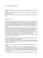


![[Nông Nghiệp] Trồng Xoài, Na, Đu Đủ, Hồng Xiêm - Gs.Ts.Trần Thế Tục phần 4 pdf](https://media.store123doc.com/images/document/2014_07/13/medium_hva1405268444.jpg)
![[Công Trình Cao Tầng] Công Nghệ Ván Khuôn Trượt - Bùi Mạnh Hùng phần 4 pdf](https://media.store123doc.com/images/document/2014_07/13/medium_joi1405268447.jpg)
![[Xây Dựng] Giáo Trình Hệ Thống Đường Ống Cấp Thoát Nước - Ks.Đỗ Trọng Miên phần 4 pdf](https://media.store123doc.com/images/document/2014_07/14/medium_mfj1405275660.jpg)