Physical Processes in Earth and Environmental Sciences Phần 5 pptx
Bạn đang xem bản rút gọn của tài liệu. Xem và tải ngay bản đầy đủ của tài liệu tại đây (1.89 MB, 34 trang )
122 Chapter 4
are given as a critical value of the overall dimensionless
boundary shear stress, . The threshold value is thus an
important practical parameter in environmental engineer-
ing. A particular fluid shear velocity, u
*
, above the thresh-
old for motion may also be expressed as a ratio with
respect to the critical threshold velocity, u
*c
. This is the
transport stage, defined as the ratio u
*
/u
*c
. Once that
threshold is reached, grains may travel (Fig. 4.38) by
(1) rolling or intermittent sliding (2) repeated jumps or
saltations (3) carried aloft in suspension. Modes (1) and
(2) comprise bedload as defined previously. Suspended
motion begins when bursts of fluid turbulence are able to
lift saltating grains upward from their regular ballistic
trajectories, a crude statistical criterion being when the
mean upward turbulent velocity fluctuation exceeds the
particle fall velocity, that is, wЈ/V
p
Ͼ 1.
4.8.2 Fluids as transporting machines: Bagnold’s
approach
It is axiomatic that sediment transport by moving fluid
must be due to momentum transfer between fluid and
sediment and that the resulting forces are set up by the
t
zz
t
zx
Suspended
load
Bedload
Bed
z
x
Fig. 4.34 Stresses responsible for sediment transport.
Wind flow
Lift
Drag
Surface
Note decay of pressure lift force to
zero at >3 sphere diameters away
from surface as the Bernoulli
effect is neutralized by
symmetrical flow above and
below the sphere
z
x
Fig. 4.35 Relative magnitude of shear force (drag) and pressure lift
force acting on spheres by constant air flow at various heights above
a solid surface.
Fig. 4.36 (left) W.S. Chepil made the quantitative measurements of
lift and drag used as a basis for Fig. 4.35. Here he is pictured
adjusting the test section of his wind tunnel in the 1950s. Much
research into wind blown transport in the United States was
stimulated by the Midwest “dust bowl” experiences of the 1930s.
10
–1
10
–0
10
–2
10
–2
10
–1
10
0
10
1
10
2
10
3
10
4
Grain Reynolds number, u
*
d/n
Dimensionless bed shear stress,
u = t/(s–r)gd
Envelope of data
Fig. 4.37 Variation of dimensionless shear stress threshold, , for sediment motion in water flows as a function of grain Reynolds number. is
known as the Shields function, after the engineer who first proposed it in the 1930s.
LEED-Ch-04.qxd 11/26/05 13:29 Page 122
Flow, deformation, and transport 123
differential motion of the fluid over an initially stationary
boundary. Working from dynamic principles Bagnold
assumed that
1 In order to move a layer of stationary particles, the layer
must be sheared over the layer below. This process involves
lifting the immersed mass of the topmost layer over the
underlying grains as a dilatation (see Section 4.11.1), hence
work must be done to achieve the result.
2 The energy for the transport work must come from the
kinetic energy of the shearing fluid.
3 Close to the bed, fluid momentum transferred to any
moving particles will be transferred in turn to other sta-
tionary or moving particles during impact with the loose
boundary; a dispersion of colliding grains will result.
The efficacy of particle collisions will depend upon the
immersed mass of the particles and the viscosity of
the moving fluid (imagine you play pool underwater).
4 If particles are to be transported in the body of the fluid
as suspended load, then some fluid mechanism must act to
effect their transfer from the bed layers. This mechanism
must be sought in the processes of turbulent shear,
chiefly in the bursting motions considered previously
(Section 4.5).
The fact that fluids may do useful work is obvious from
their role in powering waterwheels, windmills, and tur-
bines. In each case flow kinetic energy becomes machine
mechanical energy. Energy losses occur, with each machine
operating at a certain efficiency, that is, work rate ϭ avail-
able power ϫ efficiency. Applying these basic principles to
nature, a flow will try to transport the sediment grains
supplied to it by hillslope processes, tributaries, and bank
erosion. The quantity of sediment carried will depend
upon the power available and the efficiency of the energy
transfer between fluid and grain.
4.8.3 Some contrasts between sediment transport in
air and water flows
Although both air and water flows have high Reynolds
numbers, important differences in the nature of the two
transporting systems arise because of contrasts in fluid
material properties. Note in particular that
1 The low density of air means that air flows set up lower
shearing stresses than water flows. This means that the com-
petence of air to transport particles is much reduced.
2 The low buoyancy of mineral particles in air means
that conditions at the sediment bed during sediment
transport are dominated by collision effects as particles
exchange momentum with the bed. This causes a fraction
of the bed particles to move forward by successive grain
impacts, termed creep.
3 The bedload layer of saltating and rebounding grains
is much thicker in air than water and its effect adds signif-
icant roughness to the atmospheric boundary layer.
4 Suspension transport of sand-sized particles by the
eddies of fluid turbulence (Cookie 13) is much more
Lift
Drag
Gravity
Resultant
Pivot
angle
Impact
Lift off
Saltation trajectory
Flow
Suspension
trajectory
Turbulent
burst
Grain lifted aloft by
turbulent
burst
z
x
Fig. 4.38 Grain motion and pathways.
Table 4.3 Some physical contrasts between air and water flows.
Material or flow property Air Water
Density, (kg m
Ϫ3
) at STP 1.3 1,000
Sediment/fluid density ratio 2,039 2.65
Immersed weight of sediment per unit volume (N m
Ϫ3
) 2.6 и10
4
1.7 и10
4
Dynamic viscosity, (Ns m
Ϫ2
) 1.78 и10
Ϫ5
1.00 и10
Ϫ3
Stokes fall velocity,
V
p
(m s
Ϫ1
) for a 1 mm particle ~8 ~0.15
Bed shear stress,
zx
(N m
Ϫ2
) for a 0.26 m s
Ϫ1
~0.09 ~68
shear velocity
Critical shear velocity,
u
*c
, needed to 0.35 0.02
move 0.5 mm diameter sand
LEED-Ch-04.qxd 11/26/05 13:29 Page 123
124 Chapter 4
difficult in air than in water, because of reduced fluid shear
stress and the small buoyancy force. On the other hand the
widespread availability of mineral silt and mud (“dust”)
and the great thickness of the atmospheric boundary layer
means that dust suspensions can traverse vast distances.
5 Energetic grain-to-bed collisions mean that wind-
blown transport is very effective in abrading and rounding
both sediment grains and the impact surfaces of bedrock
and stationary pebbles.
4.8.4 Flow, transport, and bedforms in
turbulent water flows
As subaqueous sediment transport occurs over an initially
flat boundary, a variety of bedforms develop, each adjusted
to particular conditions of particle size, flow depth and
applied fluid stress. These bedforms also change the local
flow field; we can conceptualize the interactions between
flow, transport, and bedform by the use of a feedback
scheme (Fig. 4.39).
Current ripples (Fig. 4.40c) are stable bedforms above
the threshold for sediment movement on fine sand beds at
relatively low flow strengths. They show a pattern of flow
separation at ripple crests with flow reattachment down-
stream from the ripple trough. Particles are moved in bed-
load up to the ripple crest until they fall or diffuse from the
separating flow at the crest to accumulate on the steep rip-
ple lee. Ripple advance occurs by periodic lee slope
avalanching as granular flow (see Section 4.11). Ripples
form when fluid bursts and sweeps to interact with the
boundary to cause small defects. These are subsequently
Turbulent
flow
Bedform
Transport
Turbulent
flow structures
Modifications
(+ve and –ve) to
turbulence intensity
Local transport rate
Bedform initiation and development
1 ry causes
2 ry feedback
Flow separation,
shear layer eddies,
outer flow modification
Fig. 4.39 The flow–transport–bedform “trinity” of primary causes and secondary feedback.
(b)
(c)
(a)
Fig. 4.40 Hierarchy of bedforms revealed on an estuarine tidal bar becoming exposed as the tidal level falls. (a) Air view of whole bar from
Zeppelin. Light colored area with line (150 m) indicates crestal dunes illustrated in (b). (b) Dunes have wavelengths of 5–7 m and heights of
0.3–0.5 m. (c) Detail of current ripples superimposed on dunes, wavelengths c.12–15 cm.
LEED-Ch-04.qxd 11/26/05 13:38 Page 124
Flow, deformation, and transport 125
enlarged by flow separation processes. Ripples do not form
in coarse sands (d Ͼ 0.7 mm); instead a lower-stage plane
bed is the stable form. The transition coincides with disrup-
tion of the viscous sublayer by grain roughness and the
enhancement of vertical turbulent velocity fluctuations. The
effect of enhanced mixing is to steepen the velocity gradient
and decrease the pressure rise at the bed in the lee of defects
so that the defects are unable to amplify to form ripples.
With increasing flow strength over sands and gravels, cur-
rent ripples and lower-stage plane beds give way to dunes.
These large bedforms (Fig. 4.40a, b) are similar to current
ripples in general shape but are morphologically distinct,
with dune size related to flow depth. The flow pattern over
dunes is similar to that over ripples, with well-developed
flow separation and reattachment. In addition, large-scale
advected eddy motions rich in suspended sediment are gen-
erated along the free-shear layer of the separated flow. The
positive relationship between dune height, wavelengths, and
flow depth indicates that the magnitude of dunes is related
to thickness of the boundary layer or flow depth.
As flow strength is increased further over fine to coarse
sands, intense sediment transport occurs as small-amplitude/
long wavelength bedwaves migrate over an upper-stage
plane bed.
Antidunes are sinusoidal forms with accompanying in
phase water waves (Fig. 4.41) that periodically break and
move upstream, temporarily washing out the antidunes.
They occur as stable forms when the flow Froude number
(ratio between velocity of mean flow and of a shallow
water wave, that is, u/(gd)
0.5
) is Ͼ0.84, approximately
indicative of rapid (supercritical) flow, and are thus com-
mon in fast, shallow flows. Antidune wavelength is related
to the square of mean flow velocity.
(a)
(b)
Fig. 4.41 Fast, shallow water flow (flow right to left; Froude number
Ͼ 0.8) over sand to show downstream trend from (a) in-phase
standing waves over antidune bedforms, to (b) downstream to
upstream-breaking waves. In the next few seconds the breaking
waves propagate into area (a). The standing waves subsequently
reform over the whole field and thereafter the upstream-breaking
cycle begins again.
4.9 Waves and liquids
Waves are periodic phenomena of extraordinarily diverse
origins. Thus we postulate the existence of sound and elec-
tromagnetic waves, and directly observe waves of mass
concentration each time we enter and leave a stationary or
slowly moving traffic jam. A great range of waveforms
transfer energy in both the atmosphere and oceans, with
periods ranging from 10
Ϫ2
to 10
5
s for ocean waves. They
transfer energy and, sometimes, mass. The commonest vis-
ible signs of fluid wave motion are the surface waveforms
of lakes and seas. Many waveforms are in lateral motion,
traveling from here to there as progressive waves, although
some are of too low frequency to observe directly, like the
tide. Yet others are standing waves, manifest in many
coastal inlets and estuaries. In the oceans, waves are usually
superimposed on a flowing tidal or storm current of
greater or lesser strength. Such combined flows carry attrib-
utes of both wave and current but the combination is more
complex than just a simple addition of effects (Section 4.10).
Waves also occur at density interfaces within stratified
fluids as internal waves, as in the motion along the
oceanic, thermocline, oceanic, and shelf margin tides,
density and turbidity currents. We must also note the
astonishing solitary waves seen as tidal bores and reflected
density currents.
4.9.1 Deep water, surface gravity waves
“Deep” in this context is a relative term and is formally
defined as applying when water depth, h, is greater than a
half wavelength, that is, h Ͼ /2 (Fig. 4.42). Deep water
waves at the sea or lake surface are more-or-less regular
periodic disturbances created by surface shear due to
blowing wind. The stationary observer, fixing their gaze at
a particular point such as a partially submerged marker
post, will see the water surface rise and fall up the post as a
wave passes by through one whole wavelength. This rise
and fall signifies the conversion of wave potential to kinetic
energy. The overall wave shape follows a curve-like, sinu-
soidal form and we use this smoothly varying property as a
LEED-Ch-04.qxd 11/26/05 13:38 Page 125
126 Chapter 4
simple mathematical guide to our study of wave physics
(Cookie 14). It is a common mistake to imagine deep
water waves as heaps and troughs of water moving along a
surface: it is just wave energy that is transferred, with no
net forward water motion.
The simplest approach is to set the shape of the wave-
form along an xz graph and consider that the periodic
motion of z will be a function of distance x, wave height,
H, wavelength, , and celerity (wave speed), c. Attempts to
investigate wave motion in a more rigorous manner
assume that the wave surface displacement may be approx-
imated by curves of various shapes, the simplest of which is
a harmonic motion used in linear (Airy) wave theory
(Cookie 14). Sinusoidal waves of small amplitude in deep
water cause motions that cannot reach the bottom. Small-
amplitude wave theory approach assumes the water is
inviscid and irrotational. The result shows that surface
gravity waves traveling over very deep water are dispersive
in the sense that their rate of forward motion is directly
dependant upon wavelength: wave height and water depth
play no role in determining wave speed (Fig. 4.42). An
important consequence of dispersion is that if a variation
of wavelength occurs among a population of deep water
waves, perhaps sourced as different wave trains, then the
longer waves travel through the shorter ones, tending to
amplify when in phase and canceling when out of phase.
This causes production of wave groups, with the group
speed, c
g
being 50 percent less than the individual wave
speeds, c (Cookie 15).
At any fixed point on or within the water column the
fluid speed caused by wave motion remains constant while
the direction of motion rotates with angular speed, ; and
any particle must undergo a rotation below deep water
waves (Fig. 4.42). The radii of these water orbitals as they
are called, decreases exponentially below the surface.
4.9.2 Shallow water surface gravity waves
Deep water wave theory fails when water depth falls below
about 0.5. This can occur even in the deepest oceans for
the tidal wave and for very long (10s to 100s km) wave-
length tsunamis (see below). Shallow water waves are
quite different in shape and dynamics from that predicted
by the simple linear theory of sinusoidal deep water waves.
As deep water waves pass into shallow water, defined as
h Ͻ /20, they suffer attenuation through bottom friction
and significant horizontal motions are induced in the
developing wave boundary layer (Figs 4.43 and 4.44). The
waves take on new forms, with more pointed crests and
flatter troughs. After a transitional period, when wave
speed becomes increasingly affected by water depth,
shallow-water gravity waves move with a velocity that is
proportional to the square root of the water depth, inde-
pendent of wavelength or period (Cookie 16). The disper-
sive effect thus vanishes and wave speed equals wave group
speed. The wave orbits are elliptical at all depths with
increasing ellipticity toward the bottom, culminating at
the bed as horizontal straight line flow representing to-
and-fro motion. Steepening waves may break in very shal-
low water or when intense wind shear flattens wave crests
(Section 6.6). In both cases air is entrained into the surface
l
Crest
Trough
Still water
level
y
Depth, h,
> l/2
x
Wave
advance
H
y = H sin vt
For simple harmonic motion of
angular velocity, v, the
displacement of the still water
level over time, t, is given by:
Wave speed, c
The equations of motion for
an inviscid fluid can be solved
to give the following useful
expression for wave speed, c:
Every water
particle rotates
about a
time-mean
circular motion
Arrows show instantaneous
motion vectors at each
arrowhead
Since the coefficients are
constant, for SI units we have:
c = gl / 2p
c = 1.25 l
Fig. 4.42 Deep water wave parameters, circular orbitals, and instantaneous water motion vectors. Deep water waves are sometimes called short
waves because their wavelengths are short compared to water depth.
Note: In nature, individual waves pass through wave groups traveling at speed C
Ϫ
2
with energy transmitting at this rate.
LEED-Ch-04.qxd 11/26/05 13:38 Page 126
Flow, deformation, and transport 127
boundary layer of the water as the water collapses or spills
down the wave front, thus markedly increasing the air-
to-sea-to-air transfer of momentum, thermal energy,
organo-chemical species, and mass. The production of
foam and bubble trains is also thought to feed back to the
atmospheric boundary layer itself, leading to a marked
reduction of boundary layer roughness and therefore fric-
tion in hurricane force winds (Section 6.2).
4.9.3 Surface wave energy and radiation stresses
The energy in a wave is proportional to the square of its
height. Most wave energy (about 95 percent) is concen-
trated in the half wavelength or so depth below the mean
water surface. It is the rhythmic conversion of potential to
kinetic energy and back again that maintains the wave
motion; derivations of simple wave theory are dependent
upon this approach (Cookies 14 and 16). The displace-
ment of the wave surface from the horizontal provides
potential energy that is converted into kinetic energy by
the orbital motion of the water. The total wave energy per
unit area is given by E ϭ 0.5ga
2
, where a is wave ampli-
tude (ϭ0.5 wave height H). Note carefully the energy
dependence on the square of wave amplitude. The energy
flux (or wave power) is the rate of energy transmitted in
the direction of wave propagation and is given by ϭ Ecn,
where c is the local wave velocity, and the coefficients are
n ϭ 0.5 in deep water and n ϭ 1 in shallow water. In deep
water the energy flux is related to the wave group velocity
rather than to the wave velocity. Because of the forward
energy flux, Ec, associated with waves approaching the
shoreline, there exists also a shoreward-directed momen-
tum flux or stress outside the zone of breaking waves. This
is termed radiation stress and is discussed in Section 6.6.
4.9.4 Solitary waves
Especially interesting forms of solitary waves or bores may
occur in shallow water due to sudden disturbances affect-
ing the water column. These are very distinctive waves of
translation, so termed because they transport their con-
tained mass of water as a raised heap, as well as transporting
the energy they contain (Fig. 4.45). These amazing fea-
tures were first documented by J.S. Russell who came
across one in 1834 on the Edinburgh–Glasgow canal in
central Scotland. Here are Russell’s own vivid words,
Depth, h,
< λ /20
Every water particle rotates
about a time-mean ellipsoidal
motion, the ellipses becoming
more elongated with depth
The waves move with a velocity
proportional to the square root
of the water depth, independent
of the wavelength or period:
c = gh
Fig. 4.43 Shallow water waves and their ellipsoidal orbitals. Shallow water waves are sometimes called long waves because their wavelengths are
long compared to water depths. Note that the orbital motions flatten with depth but do not change in maximum elongation.
Note: All waves in similar water depths travel at the same speed and transmit their energy flux at this rate.
Fig. 4.44 Time-lapse photograph of shallow water wave orbitals visualized by tracer particle. This flow visualization of suspended particles was
photographed under a shallow water wave traversing one wavelength, , left to right. Wave amplitude is 0.04 and water depth is 0.22. The
clockwise orbits are ellipses having increasing elongation toward the bottom. Some surface loops show slow near-surface drift to the right.
This is called Stokes drift and is due to the upper parts of orbitals having a greater velocity than the lower parts and to bottom friction. The
surface drift is accompanied by compensatory near-bed drift to the left, due to conservation of volume in the closed system of the experimental
wave tank. Stokes drift without the added effects of bottom friction also occurs in short, deep water waves.
LEED-Ch-04.qxd 11/26/05 13:39 Page 127
128 Chapter 4
written in 1844:
I happened to be engaged in observing the motion of a vessel at
a high velocity, when it was suddenly stopped, and a violent and
tumultuous agitation among the little undulations which the ves-
sel had formed around it attracted my notice. The water in vari-
ous masses was observed gathering in a heap of a well-defined
form around the centre of the length of the vessel. This accumu-
lated mass, raising at last to a pointed crest, began to rush for-
ward with considerable velocity towards the prow of the boat,
and then passed away before it altogether, and, retaining its form,
appeared to roll forward alone along the surface of the quiescent
fluid, a large, solitary, progressive wave. I immediately left the
vessel, and attempted to follow this wave on foot, but finding its
motion too rapid, I got instantly on horseback and overtook it in
a few minutes, when I found it pursuing its solitary path with a
uniform velocity along the surface of the fluid. After having fol-
lowed it for more than a mile, I found it subside gradually, until
at length it was lost among the windings of the channel.
Briefly, a solitary wave is equivalent to the top half of a
harmonic wave placed on top of undisturbed fluid, with all
the water in the waveform moving with the wave; such
bores, unlike surface oscillatory gravity waves, transfer
water mass in the direction of their propagation.
Somewhat paradoxically we can also speak of trains of soli-
tary waves within which individuals show dispersion due to
variations in wave amplitude. They propagate without
change of shape, any higher amplitude forms overtaking
lower forms with the very remarkable property, discovered
in the 1980s, that, after collision, the momentarily com-
bining waves separate again, emerging from the interaction
with no apparent visible change in either form or velocity
(Fig. 4.46). Such solitary waves are called solitons.
4.9.5 Internal fluid waves
Within the oceans there exist sharply-defined sublayers of
the water column which may differ in density by only small
amounts (Fig. 4.47). These density differences are com-
monly due to surface warming or cooling by heat energy
transfer to and from the atmosphere by conduction. They
may also be due to differences in salinity as evaporation
occurs or as freshwater jets mix with the ambient ocean
mass. The density contrast between layers is now small
enough (in the range 3–20 kg m
Ϫ3
, or 0.003–0.02) so that
the less dense and hence buoyant surface layers feel the
drastic effects of reduced gravity. Any imposed force caus-
ing a displacement and potential energy change across the
sharp interface between the fluids below the surface is now
opposed by a reduced gravity (Section 3.6) restoring force,
gЈϭ(⌬/)g. The wave propagation speed, is
now reduced in proportion to this reduced gravity, to
, while the wave height can be very much larger.
Internal waves of long period and high amplitude progres-
sively “leak” their energy to smaller length scales in an
energy “cascade,” causing turbulent shear that may
c ϭ ͙g
Ј
h
c ϭ ͙gh
Fig. 4.45 Solitary waves: Russell’s original sketch to illustrate the
formation and propagation of a solitary wave. You can achieve the
same effect with a simple paddle in a channel, tank, or bath. The
solitary wave is raised as a “hump” of water above the general
ambient level. The “hump” is thus transported as the excess mass
above this level, as well as by the kinetic energy it contains by virtue
of its forward velocity, c.
Solitons in shallow water
A
AЈ
A
AЈ
B
BЈ
C
CЈ
B
BЈ
t = 0
t = +1 s
Fig. 4.46 Solitary wave A–AЈ has just formed as a reflected wave from a harbor wall behind and to the left. The views show the wave moving
forward (c ϭ 1 m s
Ϫ1
) through incoming shallow water waves B–BЈ and C–CЈ with little deformation or diminution.
LEED-Ch-04.qxd 11/26/05 13:39 Page 128
Flow, deformation, and transport 129
ultimately cause the waves to break. This is an important
mixing and dissipation mechanism for heat and energy in
the oceans (Section 6.4.4).
4.9.6 Waves at shearing interfaces –
Kelvin–Helmholtz instabilities
Stratified fluid layers (Section 4.4) may be forced to shear
over or past one another (Fig. 4.48). Such contrasting
flows commonly occur at mixing layers where water masses
converge; fine examples occur in estuaries or when river
tributaries join. On a larger scale they occur along the mar-
gins of ocean currents like the Gulf Stream (see Section 6.4).
In such cases an initially plane shear layer becomes unsta-
ble if some undulation or irregularity appears along the
layer, for any acceleration of flow causes a pressure drop
(from Bernoulli’s theorem) and an accentuation of the dis-
turbance (Fig. 4.48). Very soon a striking, more-or-less
regular, system of asymmetrical vortices appears, rotating
about approximately stationary axes parallel to the plane of
shear. These vortices are important mixing mechanisms in
nature; they are called Kelvin–Helmholtz waves.
4.9.7 The tide: A very long period wave
The tide, a shallow-water wave of great speed
(20–200 ms
Ϫ1
) and long wavelength, causes the regular
rise and fall of sea level visible around coastlines. Newton
was the first to explain tides from the gravitational forces
acting on the ocean due to the Moon and Sun (Figs
4.49–4.52). Important effects arise when the Sun and
Moon act together on the oceans to raise extremely high
tides (spring tides) and act in opposition on the oceans to
raise extremely low tides (neap tides) in a two-weekly
rhythm. It has become conventional to describe tidal
ranges according to whether they are macrotidal (range
Ͼ4 m), mesotidal (range 2–4 m), or microtidal (range
Ͻ2 m), but it should be borne in mind that tidal
range always varies very considerably with location in any
one tidal system.
An observer fixed with respect to the Earth would
expect to see the equilibrium tidal wave advance progres-
sively from east to west. In fact, the tides evolve on a rotat-
ing ocean whose water depth and shape are highly variable
with latitude and longitude. The result is that discrete
rotary and standing waves dominate the oceanic tides and
their equivalents on the continental shelf (see Section 6.6).
In detail the nature of the tidal oscillation depends criti-
cally on the natural periods of oscillation of the particular
ocean basin. For example, the Atlantic has 12-h tide-
forming forces while the Gulf of Mexico has 24 h. The
Pacific does not oscillate so regularly and has mixed tides.
Advance of the tidal wave in estuaries that narrow
upstream is accompanied by shortening parallel to the crest,
crestal amplification, and steepening of the tidal wave whose
ultimate form is that of a bore, a form of solitary wave. In a
closed tidal basin a standing wave of characteristic resonant
period, T, with a node of no displacement in the middle and
antinodes of maximum displacement at the ends, has a
Atmosphere
Warm/fresh upper water layer
Cool/saline lower layer
r
1
r
2
h
1
h
2
h
l
H
Wave motions propagating down
Wave motions propagating up from depth
Waves may
break and
mix
Fig. 4.47 Internal waves at a sharp density interface.
Initial configuration
Intermediate
+
+
−−
+
+
−
−
Fig. 4.48 Kelvin–Helmholtz waves formed at a sharp, shearing interface between clear up-tank moving less dense fluid and dark downtank-
moving denser fluid. Note shape of waves, asymmetric upflow. Pressure deviations from Bernoulli accelerations amplify any initial disturbances
into regular vortices.
LEED-Ch-04.qxd 11/26/05 13:40 Page 129
130 Chapter 4
wavelength, , twice the length, L, of the basin. The speed
of the wave is thus 2L/T and, treating the tidal wave as a
shallow-water wave, we may write Merian’s formula as
. T is now given by . When the period
of incoming wave equals or is a certain multiple of this reso-
nant period, then amplification occurs due to resonance, but
with the effects of friction dampening the resonant amplifi-
cation as distance from the shelf edge increases. The tide
2L/͙gh
2L/T ϭ ͙gh
occurs as a standing wave off the east coast of North
America, where tidal currents are zero in the nodal center of
the oscillating water near the shelf edge and maximum at the
margins (antinodes) where the shelf is broadest.
4.9.8 A note on tsunami
The horrendous Indian Ocean tsunami of December 2004
focused world attention on such wave phenomenon.
Tsunami is a Japanese term meaning “harbor wave.”
Tsunami is generated as the sea floor is suddenly deformed
E
Cm
Earth
Moon
As seen from the pole star, our moon
rotates anticlockwise around its common
center of mass with the Earth, Cm, every
27. 3 days
This is the path of motion
(assumed circular here) of
constant radius described by
the Earth–Moon system as it
rotates about Cm
4,700 km
M
Fig. 4.49 Revolution of the Earth–Moon pair.
E
Cm
Earth
F
c
F
c
to
Moon
Fig. 4.50 The centripetal acceleration (see Section 3.7) causes and
the centrifugal force, F
c
, directed parallel to EM of the same magni-
tude occur everywhere on the surface of the Earth.
E
Earth
Moon
M
The resultant tide-producing forces
Fig. 4.51 The gravitational attraction of the Moon on the Earth varies according to the inverse of the distance squared of any point on the Earth’s
surface from M, the center of mass of the Moon. Hence the resultant of the centrifugal and gravitational forces is the tide-producing force.
Earth
Moon
Assuming a water-covered planetary surface this is the tidal bulge
under which the Earth rotates twice daily, giving rise to two periods
of low and high water each day – the diurnal equilibrium tide
but of course the contribution of the Sun´s mass, the variation
of planetary orbits and oceanic topography make the ACTUAL
tide a
g
reat deal more com
p
licated!
E
M
Fig. 4.52 The magnitude of the tide producing force is only about 1 part in 10
5
of the gravitational force. We are interested only in the hori-
zontal component of this force that acts parallel to the surface of the ocean. This component is the tractive force available to move the oceanic
water column and it is at a maximum around small circles subtending an angle of about 54Њ to the center of Earth. The tractive force is at a
minimum along the line EM connecting the Earth–Moon system. An equilibrium state is reached, the equilibrium tide, as an ellipsoid repre-
senting the tendency of the oceanic waters flowing toward and away from the line EM. Combined with the revolution of the Earth this causes
any point on the surface to experience two high water and two low water events each day, the diurnal equilibrium tide.
LEED-Ch-04.qxd 11/26/05 13:40 Page 130
Flow, deformation, and transport 131
by earthquake motions or landslides; the water motion
generated in response to deformation of the solid bound-
ary propagate upward and radially outward to generate
very long wavelength (100s km) and long period (Ͼ60 s)
surface wave trains. By very long we mean that wavelength
is very much greater than the oceanic water depth and
hence the waves travel at tremendous speed, governed by
the shallow water wave equation . For example,
such a wave train in 3,000 m water depth gives wave
speeds of order 175 m s
Ϫ1
or 630 km h
Ϫ1
. Tsunami wave
height in deep-water is quite small, perhaps only a few
decimeters. The smooth, low, fast nature of the tsunami
wave means wave energy dissipation is very slow, causing
very long (could be global) runout from source. As in shal-
low water surface gravity waves at coasts, tsunami respond
to changes in water depth and so may curve on refraction
in shallow water. Accurate tsunami forecasting depends on
the water depth being very accurately known, for example,
in the oceans a wave may travel very rapidly over shallower
water on oceanic plateau. During run-up in shallow coastal
waters, tsunami wave energy must be conserved during
very rapid deceleration: the result is substantial vertical
amplification of the wave to heights of tens of meters.
4.9.9 Flow and waves in rotating fluids
We saw in Section 3.7 what happens in terms of radial cen-
tripetal and centrifugal forces when fluid is forced to turn
in a bend. In Section 3.8 we explored the consequences of
free flow over rotating spheres like the Earth when varia-
tions in vorticity create the Coriolis force which acts to
turn the path of any slow-moving atmospheric or oceanic
current loosely bound by friction (geostrophic flows). A
simple piece of kit to study the general nature of rotating
flows was constructed by Taylor in the 1920s, based upon
the Couette apparatus for determining fluid viscosity
between two coaxial rotating cylinders. This consisted of
two unequal-diameter coaxial cylinders, one set within the
other, the outer, larger cylinder is transparent and fixed
while the smaller, inner one of diameter r
i
is rotated by an
electric motor at various angular speeds, ⍀. The annular
space, diameter d, between the cylinders is filled with
c ϭ ͙gh
liquid of density, , and molecular viscosity, , and a small
mass of neutrally buoyant and reflective tracer particles. As
the inner cylinder rotates it exerts a torque on the liquid in
the annular space, causing a boundary layer to be set up so
that the fluid closest to the outer wall rotates less rapidly
than that adjacent to the inner wall. At very low rates of
spin nothing remarkable happens but as the spin is
increased a number of regularly spaced zonal (toroidal)
rings, termed Taylor cells, form normal to the axis of the
cylinders (Fig. 4.53); then, at some critical spin rate these
begin to deform into wavy meridional vortices. These
begin to form at a critical inner cylinder rotational
Reynolds number, Re
i
ϭ r
i
⍀d/, of about 100–120, with
the 3D wave like instabilities beginning at Re
i
Ͼ 130–140.
At high rates of spin the flow becomes turbulent, the 3D
wavy structure is suppressed and the Taylor ring structure
becomes dominant once more. Taylor cell vortex motions
involve separation of the flow into pairs of counter rotating
vortex cells.
(a)
(b)
Fig. 4.53 Taylor vortices produced in Couette apparatus (a) Regularly-
spaced toroidal Taylor vortices and (b) Wavy Taylor vortices.
4.10 Transport by waves
4.10.1 Transport under shallow water surface gravity waves
The previous sections made it clear that a sea or lake bed
under shallow water surface gravity waves is subject to an
oscillatory pattern of motion (Fig. 4.54). As the velocity of
this motion increases, sediment is put into similar motion.
Experiments reveal that once the threshold for motion is
passed then the sediment bed is molded into a pattern of
LEED-Ch-04.qxd 11/26/05 13:41 Page 131
132 Chapter 4
ripple forms, termed wave-formed or oscillatory ripples.
The wavelength and height of these ripples, of order
decimeters to centimeters respectively, reflects in a simple
way the decay in the magnitude of the oscillating flow cell
transmitted from wave surface to bed. The oscillatory flow
induces alternate formation of closed “roller” vortices in
the lee of either side of ripple crests during each forward
and backward stroke of the cycle. As the oscillatory flow
increases further in magnitude, the “up” part of each half-
stroke sends a plume of suspended sediment into the water
column (Fig. 4.55) and gradually an equilibrium suspen-
sion layer is formed that increases in thickness and concen-
tration with increasing wave power. Experiments also
reveal that wave ripples in shallow water have an inherent
“wave-drift” landward (Fig. 4.56). The ripples themselves
continuously adjust to changing wave period during
storms (Fig. 4.57) and may reach wavelengths of up to
1 m for wave periods of Ͼ10 s. At some critical junction
the increasingly 3D bed ripples are planed off and a flat
sediment bed is formed under a thick layer of suspended
sediment.
4.10.2 Transport under combined surface shallow
water surface waves and tidal currents
The observations made on transport under progressive
waves are perfectly valid for environments like lakes, but in
the shallow ocean, tidal currents of varying magnitude and
direction are invariably superimposed. These currents may
cause net transport of suspended sediment put up into the
flow by near-bed oscillatory motions. For low energy con-
ditions over smooth flow boundaries there seems to be lit-
tle overall effect of the current on near-bed values of fluid
shear stress due to the waves alone. At some critical trans-
port stage rough-bed flows show increased near-bed
vertical turbulent stresses and suspended sediment con-
centrations: it seems that some sort of interaction is set up
between the bed roughness elements, the flow, and the
oscillations.
4.10.3 Transport and mixing under internal
progressive gravity waves
Internal progressive gravity waves have important roles in
ocean water mixing and the transport and erosion of sub-
strates (Section 6.4.4). Vertical mixing occurs as internal
cccddd
The maximum horizontal orbital velocity
of a shallow water wave of surface speed
c = (gh)
0.5
, is u
max
= H/2h (gh)
0.5
,
where H = wave height and h = water
depth.
Fig. 4.54 The pattern of oscillatory motion under progressive surface shallow water gravity waves engenders a to-and-fro motion to any sea or
lake bed. Should this bed be a loose boundary of sand, gravel, or silt then bed defects cause net sediment transport and planes of divergence
(d) to convergence (c). These gradually develop into symmetrical ripple-like bedforms.
Forward stroke
Reverse stroke
Fig. 4.55 Once developed the forward and reverse portions of the
to-and-fro oscillatory motion develop flow separation on the ripple
lee side and a “jet” of suspended sediment upstream.
LEED-Ch-04.qxd 11/26/05 13:41 Page 132
Flow, deformation, and transport 133
waves break under a critical vertical gradient in imposed
shear and create turbulence. Because of the Coriolis effect
the efficacy of the resulting mixing process decreases equa-
torward. Progressive internal waves commonly develop at
the shelf edge and in fjords in summer months when shelf
waters are relatively undisturbed by storms and when ther-
mal stratification is at maximum. Erosion of fine-grained
substates by internal wave motion is thought to cause
enhanced sediment suspension that is “captured” in the
interfacial zone of influence of internal wave oscillations.
Once established, these interfacial layers of enhanced con-
centration (termed nepheloid layers) may drift shoreward
or oceanward. The density interfaces formed by the strati-
fication may trap organic suspensions stirred-up from the
bottom or derived from settling from the oceanic photic
zone above. Combined with any tendency for summer
upwelling, the sites of internal wave generation may thus
focus organic productivity.
Fig. 4.56 These oscillation wave ripples formed in sand on the bed of a laboratory channel are being generated under progressive shallow water
waves. Water depth is about two ripple wavelengths and the period of the surface waves is c.3 s. The small illuminated dots are reflected light
from a small neutrally buoyant marker particle that has been photographed stroboscopically. The pattern is noteworthy for its demonstration of
Stokes wave drift, whereby net forward motion occurs in shallow water waves. This engenders a net forward sediment transport vector and a for-
ward asymmetry to the ripple forms.
Fig. 4.57 Marta paddling beside a group of spectacular steep and linear symmetrical wave formed ripples developed on sand. The ripples
developed under storm wave conditions, probably with some amplification in the beach inlet.
4.11 Granular gravity flow
At home we are familiar with granular flow, dawdling over
the breakfast table with a jar of muesli or cereal, a pot of
sugar crystals, or a salt cellar. Each of these materials is a
granular aggregate, quite stable within its container walls
LEED-Ch-04.qxd 11/26/05 13:42 Page 133
134 Chapter 4
until tilted to a certain critical angle, upon which the
particles loose themselves from their neighbors and tum-
ble down the inclined face. We sleepily observe that the
grain aggregates must transport themselves with no help
from the surrounding fluid, in this case, air. We deduce by
observation that aggregates of particles may either be at
rest in a stable fashion or else they flow downslope like a
fluid. How does this behavior come about?
4.11.1 Reynolds again
As so often in this text we follow the pioneering footsteps
(literally damp footsteps in this case) of Reynolds, who pre-
sented basic observations and hypotheses on the problem
in 1885. Reynolds pointed out that ideal, rigid, smooth
particles had long been used to explain the dynamics of
matter and that more recently they formed the physical
basis for the kinetic theory of gases and explanations for dif-
fusion. He pointed out, however, that the natural behavior
of masses of rigid particles, exemplified as he strode over a
damp sandy beach, had a unique property not possessed by
fluids or continuous solids that “consists in a definite
change of bulk, consequent on a definite change of shape
or distortional strain, any disturbance whatever causing a
change of volume.” Reynolds’ walks across newly exposed
but still water-saturated beach sand: “When the falling tide
leaves the sand firm, as the foot falls on it the sand whitens,
or appears momentarily to dry round the foot . . . the pres-
sure of the foot causing dilatation the surface of the
water . . . lowered below that of the sand.” Let us develop
Reynolds’ concept in our own way.
4.11.2 Static properties of grains
In order to simplify the initial problem, we assume, as did
Reynolds, that the particles in question are perfectly
round spheres. We are thus dealing with macroscopic par-
ticles of a size too large to exhibit mutual attraction or
repulsion due to surface energies, as envisaged for atoms.
While at rest a mass of such particles must support itself
against gravity at the myriad of contact points between
individual grains (Fig. 4.58). We can imagine two end-
members for geometrical arrangement, the ordering or
packing, of such spheres. The maximum possible close
packing would place the spheres in cannon ball fashion,
each fitting snugly within the depression formed by the
array of neighbors below and above. By way of contrast,
the minimum possible close packing would be a more ide-
alized arrangement, difficult to obtain in practice, but
nevertheless possible, where each sphere rests exactly
above or below adjacent spheres. The reader may recog-
nize these packing arrangements as similar to those
revealed by x-ray analysis of the arrangement of atoms in
certain crystalline solids, the former termed rhombohedral
and the latter cubic.
Using these simple end-member models for ideal pack-
ing we can define an important static property of granular
aggregates. This is solid concentration, C, or fractional
packing density. Its inverse is (1 Ϫ C), defining the inter-
granular concentration, P, termed porosity or void fraction.
To calculate C we take the total volume of space occupied
by the grain aggregate as a whole, as for example in some
real or imaginary container of known volume, and express
the fraction of its space occupied by the solid grains alone.
y
1
y
1
Rhombohedral (cannonball)
Cubic
y
2
, line of contact points
for cubic packing
(a)
(b)
(c)
Grain layer
lifts up by
∆d = y
2
– y
1
Fig. 4.58 (a) Mode of granular packing epitomized by this stable pyramid of cannonballs. (b) and (c) Any displacement from condition (b) to
(c) must involve a dilatation of magnitude, ⌬d ϭ y
2
– y
1
.
LEED-Ch-04.qxd 11/26/05 13:43 Page 134
Flow, deformation, and transport 135
The minimum possible solid concentration, C ϭ 0.52, is
for cubic packing (/6) and the maximum, 0.74, is for
rhombohedral packing ( ). In practice, as
Reynolds pointed out, natural solid concentration varies
widely, but always between our upper and lower limits.
Both C and P are obviously important properties of
natural granular aggregates like sediment and sedimentary
rock. They control the ability of such aggregates to hold
fluid in their pore space, be it water in aquifers, hydro-
carbons in reservoirs, or magma melt in the crust or man-
tle. Also, the size of the pores has an important control
over rate of fluid throughflow, termed permeability
(Sections 4.13 and 6.7).
1
ր
͙2
·
ր
3
4.11.3 Conditions for a stationary aggregate to
shear and/or flow
There is only one force, gravity, that can cause the self pro-
pelled flow of grain aggregates. This may at first seem
strange because it is gravity after all that is keeping the
grain aggregate stable, by pulling each grain downward
toward its neighbors (Fig. 4.59). But, in an experiment
where we suddenly free an aggregate from a container or
containing medium, the grains flow outward, shearing,
colliding, and bouncing as they do so. So, it seems that
the aggregate as a whole has no apparent resistance to
shear! But is this not the characteristic of a fluid? How can
mg
normal
stress,
s = mg cos b
normal
stress,
s = mgcos b
shear stress,
t = mg sin b
shear stress,
t = mg sin b
b
b
(a) (b) (c)
−t
mg
normal
stress,
s =
m
t
mg
b
b
−t
m
t
b = 0
b > b
crit
b < b
crit
m = mass of grains
At equilibrium, t/s = tan b
Fig. 4.59 Conditions for grain shear. (a) Grains on a horizontal surface, (b) grains on a slope just prior to granular flow, and (c) grains shearing
on a slope during granular flow.
Granular fluids
Fig. 4.60 A random initial mixture of larger sugar crystals (dark) and glass beads from a reservoir has avalanched down a 45Њ slope,
spontaneously segregating and stratifying during transport.
LEED-Ch-04.qxd 11/26/05 13:44 Page 135
136 Chapter 4
a multitude of solid grains behave like a fluid? The answer
is that flowing fluid behavior only occurs once a critical
limit to stability has been exceeded and that it only ends
once another limit is reached. The initial condition, a ver-
tical wall of grains, was evidently in excess of the stability
limit. The final conditions, defining a conical pile of grains
with slopes resting at a certain average angle to the local
horizontal surface, were within the limit.
In order to explain these phenomena we return to
Reynolds’ packing modes (Fig. 4.58). Any shear of a
natural aggregate of grains (C Ͻ 0.74) must involve the
expansion of the volume as a whole. Take the case of an
array of spheres in perfect rhombohedral packing. These
must be sheared and raisedup by a small average distance,
⌬d, over their lower neighbors before they can shear
and/or slide off as a flowing mass; the grain mass suffers an
Fig. 4.61 An initial random mix of Riojanas beans and Valencia rice in a glass container is shaken at 3 Hz for 20 s. All the beans rise, magically,
to the surface. Physicists use such behavior to shed light on the properties of granular fluids as analogs for the kinetic theory of gases and
solids.
Fig. 4.62 Natural snow avalanches are a major hazard in mountain ski resorts. Any inclined pack of snow layers contains weak granular or
refrozen horizons which are easily disturbed by ground or air vibrations. Low friction means gravity collapse can occur and the snow pack
disintegrates into a granular flow whose equilibrium velocity may exceed 20 m s
Ϫ1
.
LEED-Ch-04.qxd 11/26/05 13:45 Page 136
Flow, deformation, and transport 137
Bagnold originally proposed that the dispersive stress is
greatest close to the basal shear plane of the granular flow
and that there, large particles exerted a higher stress (to
the square of diameter). Hence these larger particles move
upward through the flow boundary layer to equalize stress
gradients. However, a second hypothesis, termed kinetic
filtering, says that small grains simply filter through the
voids left momentarily below larger jostling grains until
they rest close to the shear plane; the larger grains must
therefore simply rise as a consequence. A simple test for
the rival hypotheses is to shear grains of equal size but con-
trasting density, since
also depends upon grain density.
It is observed that sometimes the densest grains do
indeed rise to the flow surface. Further experiments
with naturally varying grain density and size reveals vari-
able patterns of grain segregation depending on size and
density of grains and the frequency of vibration. The dis-
persive stress hypothesis is only partly confirmed by such
expansion. The expansion, Reynolds’ dilatation, of granu-
lar masses under shear, requires energy to be expended
because in effect we are having to increase the solid layer’s
potential energy by a small amount proportional to ⌬d.
Some force, an inertial one via Reynolds’ descending foot,
is required to do this. A gravity force may be more
directly imagined using a variant of Leonardo’s friction
experiment (Section 3.9), as an initially horizontal solid
body free to move rests on another fixed solid body. As
the contact between the bodies is gradually steepened a
critical energy threshold is exceeded, at a slope angle
termed the angle of static friction or initial yield,
i
. Here
the block moves downslope as the roughnesses making up
the contact surface dilatate. In the case of a loose aggre-
gate, the grains flow downslope until they accumulate as a
lower pile whose slope angle is now less than the initial
slope threshold that caused the flow to occur in the first
place. This lower slope angle, termed the angle of resid-
ual friction or shear,
r
, is usually 5–15Њ less than the ini-
tial angle of yield for natural sand grains. The value
i
Ϫ
r
gives the dilatational rotation required for shear
and flow. Some more details on the often rather compli-
cated controls on natural sand frictional behavior are
given in Cookie 17.
4.11.4 Simple collisional dynamics of granular flows
Once in motion a granular flow comprises a multitude of
grains kept in motion above a basal shear plane. An equi-
librium must be set up such that the weight force of the
grains is resisted by an equal and opposite force,
, arising
from the transfer of normal grain momentum onto the
shear plane. This concept of dispersive normal stress pro-
posed by Bagnold (Cookie 18) is analogous to the transfer
of molecular momentum against a containing wall of a ves-
sel envisaged in the kinetic theory of gases (Section 4.18).
Such normal stresses have been used to explain the fre-
quent occurrence of upward-increasing grain size, in the
deposits of granular flows (see below). Marked downslope
variations in sorting and grain size also develop sponta-
neously (Fig. 4.60): larger grains are carried further than
smaller grains because they have the largest kinetic energy.
This leads to lateral (downslope) segregation of grain size.
More interestingly, when the larger grains have higher val-
ues of , the mixture spontaneously stratifies as the smaller
grains halt first and the larger grains form an upslope-
ascending grain layer above them.
The phenomenon is popularly framed in granular
physics as the “Brazil nut problem,” or “why do Brazil
nuts rise to the top of shaken Muesli?” (Fig. 4.61).
Fig. 4.63 Sand avalanches on the steep leeside slope of a desert
dune. Here, repeated failure has occurred at the top of the dune
face: the sand has flowed downslope as a granular fluid, “stick-slip”
shearing internally to produce the observed pressure-ridges as it
does so. Shear along internal failure planes causes acoustic energy
signals to propagate, hence the “singing of the sands” that haunted
early desert explorers.
LEED-Ch-04.qxd 11/26/05 13:46 Page 137
138 Chapter 4
observations: kinetic filtering is the chief mechanism for
sorting and grain migration in multi sized granular flows,
the commonest situation in Nature.
A further intriguing complication is demonstrated by a
vibrated granular mass in a container of equal-sized grains
containing one larger grain. The vibrations induce inter-
granular collisions and a pattern of advection within the
container, with the smaller grains continuously migrating
down the walls of the container, while the larger grain, and
adjacent smaller grains move up the center. Patterns also
arise at the free surface of vibrating grain aggregates, the
newly discovered oscillons creating much interest among
physicists in the mid-1990s.
The wider environment of Earth’s surface provides
many examples of the flow of particles: witness the peri-
odic downslope movement of dune sand, screen deposits,
or the spectacular sudden triggering of powder snow or
rock avalanches (Figs 4.62 and 4.63).
4.12 Turbidity flows
As we saw in Section 3.6, buoyancy flows in general owe
their motion to forces arising from density contrasts
between local and surrounding fluid. Density contrasts
due to temperature and salinity gradients are common-
place in the atmosphere (Section 6.1) and ocean (Section
6.4) for a variety of reasons. In turbidity flows it is sus-
pended particles that cause flow density to be greater than
that of the ambient fluid. In this chapter we consider sub-
aqueous turbidity flows; we consider the equivalent class of
volcanic density currents in the atmosphere in Section 5.1.
The fluid dynamics of turbulent suspensions is a highly
complicated field because the suspended particles (1) have
a natural tendency to settle during flow, (2) affect the tur-
bulent characteristics of the flow. The trick in understand-
ing the dynamics of such flows therefore involves
understanding the means by which sediment suspension is
reached and then maintained during downslope flow and
deposition. It is probable that natural turbidity flows span
the whole spectrum of sediment concentration, but it
seems that many are dominated by suspended mud- and
silt-grade particles.
4.12.1 Origins of turbidity currents
The majority of turbidity currents probably originate by
the flow transformation of sediment slides and slumps
caused by scarp or slope collapse along continental mar-
gins (Fig. 4.64). These are often, but not invariably,
caused by earthquake shocks and are undoubtedly facili-
tated at sea level lowstands when high deposition rates
from deltas, grounding ice masses, or iceberg “graveyards”
provide ample conditions for slope collapse. A role for
methane gas hydrates in providing regional mass failure
planes in buried sediment is suspected in some cases. Slides
are thought to transform to liquefied and fluidized slumps
and then to disaggregate into visco-plastic debris flows.
These cannot transform further into turbulent suspensions
without massive entrainment of ambient seawater, and this
is not possible across the irrotational flow front of a debris
flow. Instead, debris flows must transform along their
upper edges by turbulent separation (Fig. 4.64).
Turbidity currents also form from direct underflow of
suspension-charged river water in so-called hyperpycnal
plumes, also better termed as turbidity wall jets. These have
been recorded during snowmelt floods in steep-sided basins
like fjords and glaciated lakes, in front of deltas, and in river
tributaries whose feeder channels have extremely high loads
of suspended sediments. As noted below, these freshwater
underflows may undergo spectacular behavior during the
dying stages of their evolution. Underflows are expected to
give rise to predominantly silty or muddy turbidites.
Finally, collection of sediment by longshore drift in the
nearshore heads of submarine canyons may also lead to
downslope turbidity flow. The process is most efficient
during and following storms and tends to lead to the trans-
port and deposition of sandy sediment.
4.12.2 Experimental analogs for turbidity currents
Turbidity currents are difficult to observe in nature and to
maintain in correctly-scaled laboratory experiments. We may
best illustrate their general appearance by studying saline
and scaled particle currents (Fig. 4.65) using lock-gate tanks
or continuous underflows. In the former, as the lock-gate is
removed, a surge of dense fluid moves along the horizontal
floor of the tank as a density current with well-developed
head and tail regions. Under these zero-slope conditions
the head is usually 1.5–2 times thicker than the tail, with the
ratio approaching unity as the depth of the ambient fluid
approaches the depth of the density flow. Close examination
of the head region shows it to be divided into an array of
bulbous lobes and trumpet-shaped clefts. Ambient fluid
must clearly pass into the body of the flow under the over-
hanging lobes and through the clefts. A greater mixing of
LEED-Ch-04.qxd 11/26/05 13:46 Page 138
Flow, deformation, and transport 139
denser and ambient fluid also takes place by entrainment
behind the head. Continued forward motion of the head at
constant velocity requires a transfer of denser fluid (buoy-
ancy flux) from the tail into the head (and thus for the tail to
move faster than the head) in order to compensate for
boundary friction, fluid mixing, and loss of denser fluid in
the head region. A steady state is brought about in flows
that have a near-constant input of dense solution with time.
In Nature, steady turbidity flows might occur over a
period of time as sediment-laden river water debouches
into a water body and travels along the bottom as a
continuous underflow. By way of contrast, surge-like
Curvilinear failure plane
Shear mixing around flow front
Weak layer/high pore pressure
Upslope propagation of failure
Possible
aquaplaning
Flow separation point
Free-shear layers
Separation zone,
turbulent mixing
Plastic debris flow
Head
Flow body
Turbulent mixing along free-shear layer
Turbulent flow throughout
Wall layer with
logarithmic velocity
profile
Wake
u
max
Flow ceases when slope drops below critical
slope needed to exceed Bingham yield stres
Limited (<15%) resuspension
by turbulent “pick-up”
under head and body
Turbulent suspension eventually
overtakes or diverts from debris flow
Velocit
y
of head, u
h
= 0.7(
g
´h)
0.5
Turbulent shear stress in equilibrium with bed friction due
to bedload transport and bedform development
Sediment slumps and slides
Debris flow with turbulent cap
Turbidity flow
Fig. 4.64 Various possible flow transformations from subaqueous sediment slumps and slides via debris flows to turbidity flows.
LEED-Ch-04.qxd 11/26/05 13:46 Page 139
140 Chapter 4
turbidity flows generated from finite-volume sediment
slumps or debris flows on small slopes (Ͻ1Њ) must deceler-
ate because the supply of denser fluid from behind the
head is finite and the buoyancy force driving the flow is
insufficient to overcome frictional energy losses. The head
thus shrinks until it is completely dissipated.
On slopes from at least 0.5Њ to 5Њ, head velocity of con-
tinuous underflows is independent of slope and varies
according to density contrast. Head velocity is approxi-
mately 60 percent of the tail velocity in the slope range 5Њ
to 50Њ, leading to the head increasing in size as it travels
downslope. Entrainment of ambient fluid also causes head
growth, increasingly so at higher slopes, and the momen-
tum transferred from the current to this new fluid acts as a
retarding force to counteract the buoyancy force due to
any increased slope. This “steady velocity/growing head”
behavior is also a characteristic of starting thermal plumes
but has not been investigated from the point of view of
turbidity current deposition and erosion.
Rapid dissipation of channelized turbidity flows with
consequent deposition occurs as they undergo vertical
expansion and lateral spreading on entering wide reservoirs
or basins. Such flows are wall jets, that is, aperture flows
released onto the floor of large volume reservoirs (volcanic
equivalents are discussed in Section 5.1). An interesting
transformation takes place for the case of dissipating turbid
freshwater underflows. These were particularly important in
oceanic sedimentation during the melting phases after
glaciations when vast quantities of sediment-laden freshwa-
ter were released to the oceans. In such systems, deposition
progressively reduces the buoyancy force, the bulk flow
density eventually decreases below that of sea water. The
flow comes to a complete halt, with the now positively
buoyant fluid rising upward to spread out within density
interfaces in the ocean or at the surface as a plume. The
process has been termed lofting and leads to widespread
suspension and eventual deposition of suspended muds.
4.12.3 Velocity and turbulence characteristics of
experimental turbidity flows
How quickly can dense underflows travel? We might guess
that a solution would be to treat the surge as a moving
0° 3° 6° 9°
20
20
19
132 127
120
44 56
45
44
103 147 98
106
Nose
overhang
Head
Body
Body
Fine sediment
Mixing
Mixing
(a)
(b)
Fig. 4.65 Experimental turbidity flows (photos are c.0.5 m vertical extent) traveling down progressively steeper ramps (columns of slopes
0Њ–9Њ) onto flat horizontal surfaces. (a) Turbidity flow heads (first row) and bodies (second row) on increasing ramp slopes. (b) Turbidity flow
heads (first row) and bodies (second row) on flat horizontal floors leading from upstream ramp slopes as indicated in (a).
LEED-Ch-04.qxd 11/26/05 13:46 Page 140
Flow, deformation, and transport 141
bore or shallow-water wave. If so, the conversion of potential
energy (due to mean height above the tank floor) to the
kinetic energy of motion gives the velocity of motion, u,
and proportional to the square root of water depth, h. We
might also guess that u should depend directly upon the
density difference, ⌬, between the current and the ambi-
ent fluid, or more precisely the action of reduced gravity, gЈ.
Internal velocity profiles taken through experimental
density and turbidity currents reveal a positive velocity gra-
dient in the lower part of the flows; this follows the normal
turbulent law-of-the-wall. Above a velocity maximum,
there is a negative gradient up to the top of the flow
(Fig. 4.66). The latter is due to frictional interactions
and overall retardation of the flow by the ambient fluid
in the form of production of large-scale eddies of
Kelvin–Helmholtz type. Turbulent stresses are much
increased for particulate turbidity flows over saline analogs
(Fig. 4.64).
4.12.4 Reflected density and turbidity flows
Because turbidity flows derive their motive force from the
action of gravity, they are easily influenced by submarine
slope changes. Flows may partially run up, completely run
up and overshoot, or be partially or wholly blocked,
diverted, or reflected from topographic obstacles. The
process of run-up and full or partial reflection (“sloshing”)
is particularly interesting and the effects may be seen by
inserting ramps into the kind of lock exchange tanks
described previously (Fig. 4.67). Run-up elevations are
approximately 1.5 times flow thickness and in nature it is
evident that the process can cause upslope deposition on
submarine highs. Reflection may be accompanied by the
transformation of the turbidity flow into a series of trans-
lating symmetrical waves, which have the properties of
solitary waves or bores (Section 4.9). They travel back in
the up-source direction undercutting the slowly-moving
nether regions of the still-moving forward current, trans-
porting fluid and sediment mass as they do so (Fig. 4.67).
Such internal bores have little vorticity, as witnessed by
their smooth forms.
2.5
2.0
1.0
0.5
0.0
z/z
0.5
0 0.5 1.0 –4 –20246 0 1 2 3 4 0.511.52
u/u
max
w/u
max
t
xx
/u
2
max
T
ke
/u
2
max
Saline
current
Turbidity
current
u
max
Fig. 4.66 Mean velocities (u, w), turbulent stress (
xx
), and turbulent kinetic energy (T
ke
) contrasts between experimental saline and turbidity
flows of wall jet type. Dimensionless height is with reference to z
0.5
, the height at which u reaches value 0.5 u
max
.
Ramp
Residual forward flow
Bulge of fluid travels
back as internal wave
d
1
Type C, strong wave
Type B, intermediate wave
Type A, weak wave
d
1
/d
0
>3
2<d
1
/d
0
<3
1<d
1
/d
0
<2
u
u
u
d
0
Fig. 4.67 Forward turbidity flow meets opposing topographic ramp
slope and reflects back under residual forward flow as an internal
solitary wave.
LEED-Ch-04.qxd 11/26/05 13:46 Page 141
142 Chapter 4
4.12.5 Deposition from turbidity flows
Deposition from turbidity currents may be due to flow
unsteadiness or to downstream flow nonuniformity. It is
commonly thought that passage of the head is accompa-
nied by erosion. The extent of this is a little known quan-
tity of some importance in calculating the flux of bed
material into a moving flow. Clearly any extra sediment
added to the flow will cause the head of the flow to accel-
erate. Careful sediment budget studies of Holocene
deposits in the Madeira abyssal plain reveals that 12 percent
or so of turbidite volume is composed of reworked materi-
als. This converts to about an average of 43 mm of erosion
over the total areal extent of an individual deposit.
4.13 Flow through porous and granular solids
4.13.1 Flow through stationary porous solids
“Thirsty stones” are disc-shaped surfers cut from highly
porous sandstone which soak up superfluous fluid spilt
from drinks containers. The easy flow of fluid occurs
through what we call generally a porous medium. Many
subsurface fluid flows, of water, oil, and gas occur through
such media. In general the pore fluid flow is very slow
(order Ͻ10
Ϫ3
ms
Ϫ1
) and therefore laminar, so we can
entirely neglect the kinetic contribution to flow energy.
We can also neglect the effects of frictional losses at a con-
stant rate for present purposes. From the Euler–Bernoulli
energy equation (Section 3.12; Cookie 9) we are left with
the total energy available to drive pore water flow as
(p/) ϩ z ϭ⌽, termed the pore water fluid potential.
From the simple working in Fig. 4.68 we see that ⌽ is
given by the product of a constant, g, times the hydraulic
head, h. Thus for practical purposes it suffices to measure
the level, h, in stand pipes or wells and then to map the
hydraulic water surface over the area in question (see
Section 6.7.1). The pore water velocity, u, is then propor-
tional to the gradient, ٌ, of the head field, ⌽, with flow in
the direction of greatest decrease of the field. Note care-
fully that this gradient, called the hydraulic gradient, is not
the same as the gradient of hydrostatic pore pressure
(Fig. 4.68; see also Sections 3.5 and 4.1). In symbols,
u ϭ Ϫٌ⌽K, where K is the proportionality coefficient
known as the hydraulic conductivity. The expression is uni-
versally known as Darcy’s law, namd after its originator
who was intrigued by the controls of rock hydraulic pressures
on the flow of fountains in Dijon, France in the nineteenth
century. There is some similarity of form of this equation
flow in
Piezometer 1 Piezometer 2
∆h
z = 0
Reference datum
z
2
z
1
flow
out
Q
∆l
p
1
h
1
h
2
Q
p
2
From the simplified Euler–Bernoulli energy equation
we have, generally:
Φ = gz + p/r
Neglecting atmospheric pressure, for piezometer 1,
p
1
= rg (h
1
– z
1
) and therefore
Φ = gz
1
+ rg (h
1
– z
1
)/r = gh
1
Hydraulic gradient = ∆h/∆l
Fig. 4.68 An experiment similar to that conducted by M. Darcy in 1856 to determine the energy relations of flow through porous media.
LEED-Ch-04.qxd 11/26/05 13:46 Page 142
Flow, deformation, and transport 143
with that for the 1D flow of heat through solid media
(Section 4.18, Cookie 19). Like the heat conduction
equation, it is an easy matter to solve the expression for
equilibrium flow once K, a constant for a given arrange-
ment of porosity, pore shape, pore size, fluid density, and
fluid viscosity, is known. The Kozeny–Carman equation
(not developed here) offers an approximate analytical solu-
tion to determining K as a function of these variables as
long as the particle packing is random and natural homog-
enous isotropic porosity occurs.
4.13.2 Liquefaction and fluidization of granular
aggregates
We now turn to the case when the particles in saturated
granular aggregates (Section 4.11) are simply resting upon
one another under gravity, with no cementing medium
holding them together. It is possible to imagine the situa-
tion where throughflow might cause motion of the parti-
cles away from each other: the grain aggregate is then in a
state of liquefaction. For example, it is a common observa-
tion after large earthquakes that sand and water mixtures
are expelled (often violently) from the shallow subsurface
in fountains to form sand volcanoes (Fig. 4.69). Here are
the observations made by an anonymous observer of the
great New Madrid earthquake of 1811–12 in the lower
Mississippi Valley: “Great amounts of liquid spurted into
the air, it rushed out in all quarters . . . ejected to the
height from ten to fifteen feet, and in a black shower,
mixed with sand . . . The whole surface of the country
remained covered with holes, which resembled so many
craters of volcanoes.” There is also widespread evidence
for the sinking of buildings and other structures into sands
during earthquakes, recalling the Biblical adage that pre-
dates modern building regulations by some millennia.
Although earthquakes undoubtedly impose an effective
trigger mechanism for liquefaction, they are by no means
the only one. Thus eruption of sediment and water com-
monly occurs during river floods from the bases of artificial
and natural levees.
What processes lead to production of a liquid-like state
from what was previously a stable mass of water-saturated
sand? There are two ways in which such a transformation
can take place:
1 Upward displacement of fluid may be sufficient in itself to
cause overlying grains to remain in suspension by fluidization
or seepage liquefaction, conveniently defined as the process
whereby a granular aggregate is converted to a fluid by flow
through it. The fluidized suspension may be en masse or just
restricted to selected pipe-like conduits as in the New Madrid
earthquake. Fluidization in its most simple sense requires the
velocity of moving pore fluid, U
f
, to exceed the grain fall
velocity, U
p
. More generally, in order for en masse fluidization
to occur, the upward-moving fluid must exert a normal stress
f
equal to or greater than the immersed weight of any over-
lying sediment. This force is given by
f
ϭ⌬gCh, where ⌬
is effective (immersed) grain density, g is gravity, h is overlying
(a)
(b)
Fluid
velocity,
U
f
Particle
fall
velocity,
U
p
Initial condition
Fluidized aggregate ( U
p
< U
f
)
p
1
Schematic of the simple
condition for fluidization
Fig. 4.69 (a) Sand volcanoes formed in a field after liquefaction induced by an earthquake, Imperial valley, California; (b) experimental
fluidization and sudden conduit escape as a sand volcano eruption produced by water flow through a lower, more permeable, granular
bed underlying an upper less permeable bed (dark layer).
LEED-Ch-04.qxd 11/26/05 13:48 Page 143
144 Chapter 4
sediment layer thickness, and C is fractional grain concentration.
Readers may be familiar with industrial and technological uses
of fluidization, notably the passage of hot gases through pow-
dered coal beds to optimize burn efficiency. In this case gas
fluidization is often accompanied by bubble formation, which
is uncommon in liquid fluidization. Gas-induced fluidization
is thought by some to have an important role in the mainte-
nance of certain volcanic eruptive flows, notably pyroclastic
density currents (Section 5.1).
2 It may result from the temporary collapse of grain-to-
grain contacts in loosely packed sand. The grains shaken
apart are momentarily suspended in their own porewater.
The energy for granular disaggregation is provided by the
high accelerations experienced during cyclic shock caused
by earthquake ground motions (Section 4.17). Pressure
changes due to the passage of large storm waves over a
sandy or muddy (including “fluid mud”) bottom may also
cause liquefaction, as can the sudden arrival of a turbidity
current or repeated impact of feet on saturated sands on
the beach or river bed. Should the liquefied sediment be
resting on a slope, however slight, then downslope flow
will inevitably result, the flow transforming as it does so
into a debris or turbidity flow (Section 4.12). Post-
liquefaction resettlement causes a net upward displacement
of pore fluid of volume proportional to the difference in
pre- and post-liquefaction porosity. The spatial funneling of
this flow is the cause of the violent fluidization witnessed
after earthquakes (Fig. 4.69).
4.14 Fractures
In Section 3.15 the concept of brittle versus ductile behavior
was explained. Brittle behavior involves the loss of cohe-
sion in rocks when deviatoric stresses higher than the rock
resistance are applied. The planes where rocks have lost
their cohesion are called fractures. In other words the
rocks break under certain conditions and fractures are the
places where the rocks break. Nevertheless, the definition
of fractures is a little more complicated than that. Pure
brittle fractures are well-defined surfaces where the cohe-
sion has been lost, without any distortion; if we could glue
together the pieces of the broken rock, its shape would be
the same as before (Fig. 4.70a). Brittle fractures are char-
acteristic of rocks exhibiting elastic behavior and form in
the upper part of the crust (about 10 km), although sud-
den stresses can cause brittle failure in solid viscous mate-
rials (Section 3.15). There is a broad and very intriguing
transition between the brittle and ductile fields, where the
definition of fractures is not so obvious; for example the
material in Fig. 4.70b shows some ductile deformation
accompanying the fracture since some bending occurred
before the fracture was produced. In this case, joining
together the fragments of the original piece of rock will
not give the rock’s original shape. Fractures in the brittle-
ductile transition (semi-brittle behavior) often show intense
deformation where some cohesive loss is achieved in lim-
ited, non-continuous surfaces, instead of developing a well-
defined unique fracture surface. Semi-brittle fractures do
not experience a total loss of coherence on well-defined
surfaces. Further increase in ductility, but still in the brittle-
ductile transition, produces shear bands where a cohort
of oblique, lenticular-shaped, discrete fractures is formed
(tension gashes, Fig. 4.70c). Ductile shear zones are charac-
terized by intense deformation, without apparent loss of
cohesion at macroscopic scale (visual or outcrop scales),
concentrated in a fairly narrow band (2D) surrounded by
distinctively less deformed rocks (Fig. 4.70d). Such shear
zones form at deep levels in the crust.
4.14.1 Types of fractures
The first important analysis of fractures involves how the
rock bodies on either side of the fracture move. According
to this criterion they can be classified broadly into two
(a) (b)
(d)(c)
Fig. 4.70 Different kinds of shear features: (a) Pure brittle shear
fracture, (b) in the brittle–ductile transition, fractures occur after
some previous material distortion, (c) gash fractures in the
brittle–ductile transition, and (d) ductile shear zone.
LEED-Ch-04.qxd 11/26/05 13:48 Page 144
fractures are less common and become infilled by mineral
precipitates from fluid solution, forming veins. Fractures
can be observed in rock outcrops in different shapes and
varieties, the commonest features are roughly planar sur-
faces or joints. These are cracks that extend from centimeters
to hundreds of meters. They vary in shape from irregular
discontinuous fractures to almost perfectly planar features.
Regularly spaced, planar fracture surfaces showing roughly
the same orientation form a set and are called systematic
joints. On the contrary, irregular, discontinuous, arbitrarily-
orientated fractures are called nonsystematic. Different
sets of joints can be seen cutting each other in many out-
crops. As they open perpendicularly to the fracture surface,
the trajectories of the individual joints are not much
affected by others. Nonetheless, adjustments of space once
the fractures are produced may cause some minor shear
displacements along the fracture surfaces. Joint surfaces
can be smooth or show some interesting features such as
plumose structures, fringes, or conchoidal structures which
are very useful in discerning and describing fracture prop-
agation. Plumose structures are linear irregularities, some-
times curved or wavy, arranged as in a feather or fan
fashion, parting from a single point and ending in a narrow
band or fringe at both sides. The fringe is formed by an array
of discrete en échelon fractures (Fig. 4.72). Plumose struc-
tures form in the propagation direction of the cracks,
whereas conchoidal structures are formed perpendicularly to
the general direction of the plumes and can be envisaged as
discontinuities in the fracture propagation. These structures
can be in the form of steps (Fig. 4.72b), ribs, or ripples.
Sheet joints are subhorizontal fractures, having a ten-
dency to parallel the topography. This arrangement gives
two basic interpretations for their origin. First the paral-
lelism can be seen as the cause of the topography, because
the preexisting fractures are sites of weakness in the rock
and thus control denudation patterns. A more likely expla-
nation is that topography, being a shear free surface, affects
the orientation of stresses in a principal stress plane con-
taining two of the principal stresses. Either way, sheet
joints must form when the main compressive stress is hor-
izontal and the minimum compression is vertical which
happens during crustal uplift or in general compressive
tectonic settings.
Columnar joints form in lava flows and shallow intru-
sions as the rocks experience a volume loss by cooling in
discrete domains. Commonly three conjugate sets of frac-
tures develop, arranged in geometric patterns, mostly
hexagonal as in desiccation cracks in drying wet clays. The
cracks initiate at some point in the lava flow due to tensile
stresses which arise because of differences in temperature
and volume from the surface where the lava flow is cooler
Flow, deformation, and transport 145
types: extension fractures and shear fractures. Extension
fractures or Mode I fractures (Fig. 4.71a), open perpen-
dicularly to the fracture surface and do not experience any
displacement parallel to the fracture plane. By way of con-
trast, shear fractures are characterized by a noticeable dis-
placement of the blocks along or parallel to the fracture
plane (Fig. 4.71b, c). This displacement can be produced
perpendicular to the fracture edge (Mode II) or parallel to
the fracture edge (Mode III). Faults are large shear frac-
tures (surfaces extending from several meters to the scale
of plate boundaries); the term shear fracture is mostly used
for centimeter-scale fractures.
4.14.2 Extension fractures (Mode I)
Mode I fractures or extension fractures form in the princi-
pal plane of stress containing the principal axes
1
and
2
,
perpendicular to the direction of minimum stress
3
. It is
important to remember that in these surfaces there are no
shear stress components and so there is no shear move-
ment or displacement of blocks along the fracture surface.
Extension fractures do not show offsets either side of the
fracture, even at a microscopic scale. Thus extension frac-
tures form by opening or pulling apart of blocks of rock at
each side of the fracture when the tensile stress exceeds the
strength of the rock and brittle deformation occurs. Such
brittle deformation is characteristic of the upper part of the
crust. At depth, moving into a more ductile field, extension
(a)
(b)
(c)
Mode IIIMode II
Mode I
Fig. 4.71 (a) Extension fractures (Mode I) open normal to the crack,
whereas, shear fractures (b) and (c) show displacements of blocks
parallel to the fracture. Mode II shear fractures (b) move normal to
the fracture edge and Mode III (c) move parallel to the crack edge.
LEED-Ch-04.qxd 11/26/05 13:48 Page 145
146 Chapter 4
and deeper areas which are hotter and less viscous; they
then propagate forming columnar features orientated
roughly perpendicularly to the top and bottom boundaries
of the rock body, although curved patterns of the columns
are quite common (Fig. 4.73). Increments in crack propa-
gation may result in a banding normal to the columns, dis-
playing individual plumose structures like the ones
described in joints.
Gash fractures are lenticular or sigmoid fissures (both Z
and S shaped), generally filled with some mineral (most
abundantly calcite or quartz) that develop in shear zones
at the brittle-ductile transition (Fig. 4.74), where a combi-
nation of both ductile flow and brittle fracturing occurs.
Gash veins open normal to the maximum elongation
e
1
both in coaxial, homogeneous flattening (Fig. 4.75a) or
noncoaxial simple shear zones (Fig. 4.75b). In noncoaxial
shear zones a finite increment in stress gives way to a
lenticular-shaped gash fracture set, which is orientated
at an angle with respect to the shear band edges
(Fig. 4.75b). The cracks are formed parallel to the S
1
ϪS
3
plane; note that gash fractures are not previous features in
the shear band rotated by the shear, so carefully observe
their orientation with respect to the shear sense!
Remember that simple shear (see Section 3.14) is a non-
coaxial strain and that any line forming an angle different
to from the main shear direction rotates progressively as
the main axis of the stress does. That is why a subsequent
(a)
(b)
Fringe
Fringe
c.e.
Step
Plumose
structure
Fig. 4.72 (a) Joint surfaces show plumose and conchoidal structures
(c.e.) in the main crack surface, showing the propagation of the
fracture. Fringes are located at the edges of the joints and show a set
of en echelon cracks. (b) Detail of a step in a conchoidal structure,
cutting the plumose feature in a joint surface.
(a)
(b)
Fig. 4.73 (a) Columnar joints form in volcanic or subvolcanic rocks by tensile stresses developed by contraction in small domains at cooling.
(b) Joints form vertically in the surface and propagate down forming columnar features, as in the example of Devil’s Tower in the photo
(Wyoming, United States Courtersy by R. Giménez).
LEED-Ch-04.qxd 11/26/05 13:53 Page 146
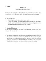
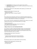


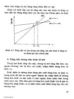
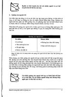


![[Địa Chất Học] Phân Loại Đất & Xây Dựng Bản Đồ Đất - TS.Đỗ Nguyên Hải phần 5 pptx](https://media.store123doc.com/images/document/2014_07/14/medium_mnd1405279205.jpg)