Physical Processes in Earth and Environmental Sciences Phần 7 pps
Bạn đang xem bản rút gọn của tài liệu. Xem và tải ngay bản đầy đủ của tài liệu tại đây (1.25 MB, 34 trang )
190 Chapter 4
4.17.6 Earthquakes and strain
In the introduction to this chapter we noted that
earthquakes were marked by release of seismic energy
along shear fracture planes. This energy is released partly
as heat and partly as the elastic energy associated with rock
compression and extension. In the elastic rebound theory
of faults and earthquakes the strain associated with tec-
tonic plate motion gradually accumulates in specific zones.
The strain is measurable using various surveying
techniques, from classic theodolite field surveys to
satellite-based geodesy. In fact, the earliest discovery of
what we may call preseismic strain was made during inves-
tigations into the causes of the San Francisco earthquake
of 1906, when comparisons were made of surveys docu-
menting c.3 m of preearthquake deformation across the
San Andreas strike-slip fault. We have already featured the
results of modern satellite-based GPS studies in decipher-
ing ongoing regional plate deformation in the Aegean area
of the Mediterranean (Section 2.4). All such geodetical
studies depend upon the elastic model of steady accumu-
lating seismic strain and displacement. But then suddenly
the rupture point (Section 3.15) is exceeded and the
strained rock fractures in proportionate or equivalent mag-
nitude to the preseismic strain. This coseismic deformation
represents the major part of the energy flux and is dissi-
pated in one or more rupture events (order 10
Ϫ2
–10
1
m
slip). The remainder dissipates over weeks or months by
aftershocks as smaller and smaller roughness elements on
the fault plane shear past each other until all the strain
energy is released. If the fault responsible breaks the
Earth’s surface then the coseismic deformation is that
measured along the exposed fault scarp whose length may
reach tens to several hundreds of kilometers.
Different types of faults give rise to characteristic first
motions of P-waves and it is this feature that nowadays
enables the type of faulting responsible for an earthquake to
be analyzed remotely from seismograms, a technique known
as fault-plane solution. Previously it was left to field surveys to
determine this, often a lengthy or sometimes impossible task.
The first arrivals in question are those up or down peaks
measured initially as the first P-wave curves on the seismo-
gram record (Fig. 4.142). It is the regional differences in the
nature of these records caused by the systematic variation of
compression and tension over the volume of rock affected by
the deformation that enables the type of faulting to be deter-
mined. This is best illustrated by a strike-slip fault where
compression and tension cause alternate zones of up (posi-
tive) or down (negative) wave motion respectively as a first
arrival wave at different places with respect to the orientation
of the fault plane responsible (Fig. 4.142). When plotted on
a conventional lower hemisphere stereonet (Cookie 19),
with shading illustrating compression, the patterns involved
are diagnostic of strike-slip faulting.
Down,
pull,
tension
Down,
pull,
tension
Up,
push,
compression
Up,
push,
compression
(b)
(c)
(a)
Fig. 4.142 To illustrate the use of first motion polarity in determining the type of fault slip, in this case the right-lateral San Andreas strike-slip
fault; (b) 1906 San Francisco quake ground displacement; (c) San Andreas dextral strike-slip fault and schematic first P-wave arrival traces.
LEED-Ch-04.qxd 11/26/05 14:08 Page 190
Flow, deformation, and transport 191
We have so far discussed flow in terms of bulk movement
and mixing but there are also a broad class of systems in
which transport of some property is achieved by differen-
tial motion of the constituent molecules that make up a
stationary system rather than by bulk movement of the
whole mass. Such systems are not quite in equilibrium, in
the sense that properties like temperature, density, and
concentration vary in space. For example, a recently erupted
lava flow cools from its surfaces in contact with the very
much cooler atmosphere and ground. A second example
might be a layer of seawater having a slightly higher salin-
ity that lies below a more dilute layer. The arrangement is
dynamically stable in the sense that the lower layer has a
negative buoyancy with respect to the upper, yet over time
the two layers tend to homogenize across their interface in
an attempt to equalize the salinity gradient at the interface.
In both examples there is a long-term tendency to equal-
ize properties. In the first it is the oscillation of molecules
along a gradient of temperature and in the second the
motion of molecules down a concentration gradient. But
how fast and why do these processes occur?
4.18.1 Gases – dilute aggregates of
molecules in motion
The gaseous atmosphere is in constant motion due to its
reaction to forces brought about by changes in environ-
mental temperature and pressure. Volcanic gases also move
in response to changes brought about by the ascent of
molten magma through the mantle and crust. When we
study the dynamics of such systems we must not only pay
attention to such bulk motions but also to those of
constituent molecules that control the pressure and
temperature variations in the gas. Compared to any speed
with which bulk processes occur, the internal motions of
stationary gases involve much higher speeds. The view of a
gas as a relatively dilute substance in which its constituent
molecules move about with comparative freedom
(Section 2.1) is reinforced by the following logic:
1 A mole of a gas molecule is the amount of mass, in
grams, equal to its atomic weight. Nitrogen thus has a
mole of mass 28 g, oxygen of 32 g, and so on. Any quan-
tity of gas can thus be expressed by the number, n, of
moles it contains.
2 A major discovery at the time when molecular theory
was still regarded as controversial, was that there are always
exactly the same number of molecules, 6 ϫ 10
23
, in one
mole of any gas. This astonishing property has come to be
known as Avagadro’s constant, N
a
, in honor of its discov-
erer. It implied to early workers in molecular dynamics that
molecules of different gases must have masses that vary
directly according to atomic weight, for example, oxygen
molecules have greater mass than nitrogen molecules.
3 Following on from Avagadro’s development, it became
obvious that Boyle’s law (Section 3.4) relating the pres-
sure, temperature, volume, and mass of gases implies that
for any given temperature and pressure, one mole of any
gas must occupy a constant volume. This is 22.4 L
(22.4 и 10
Ϫ3
m
3
) at 0°C and 1 bar.
4 It follows that each molecule of gas within a mole
volume can occupy a volume of space of some 4 и 10
Ϫ26
m
3
.
5 Typical molecules have a radius of some 10
Ϫ10
m and
may be imagined as occurring within a solid volume of
some 4и10
Ϫ30
m
3
.
From these simple considerations it seems that a gas
molecule only takes up some 10
Ϫ4
of the volume available
to it, reinforcing our previous intuition that gases are
dilute. The phenomenon of molecular diffusion in gases,
say of smell or temperature change, occurs extremely
rapidly in comparison to liquids because of the extreme
velocity of the molecules involved. Also, since gaseous
temperature can clearly vary with time, it must be the
collisions between faster (hotter) and slower (cooler)
molecules that bring about thermal equilibrium. And since
heat is a form of energy it follows that the motion of
molecules must represent the measure of a substance’s
intrinsic or internal energy, E (Section 3.4). Let us examine
these ideas a little more closely.
4.18.2 Kinetic theory – internal energy, temperature,
and pressure due to moving molecules
It is essential here to remember the distinction between
velocity, u, and speed, u. If we isolate a mass of gas in a
container then it is clear that by definition there can be no
net molecular motion, as the motions are random and will
cancel out when averaged over time (Fig. 4.143). Neither
can there be net mean momentum. In other words gas
molecules have zero mean velocity, u ϭ 0. However, the
randomly moving individual molecules have a mean
speed, u, and must possess intrinsic momentum and there-
fore also mean kinetic energy, E. In a closed volume of any
gas the idea is that molecules must be constantly bom-
barding the walls of the container – the resulting transfer
4.18 Molecules in motion: kinetic theory, heat conduction, and diffusion
LEED-Ch-04.qxd 11/26/05 14:08 Page 191
192 Chapter 4
or flux of individual molecular momentum is the origin of
gaseous pressure, temperature, and mean kinetic energy
(Fig. 4.144). These properties arise from the mean speed
of the constituent molecules: every gas possesses its own
internal energy, E, given by the product of the number of
molecules present times their mean kinetic energy. In a
major development in molecular theory, Maxwell calcu-
lated the mean velocity of gaseous molecules by relating it
to a kinetic version of the ideal gas laws, together with a
statistical view of the distribution of gas molecular speed.
The resulting kinetic theory of gases depends upon the
simple idea that randomly moving molecules have a proba-
bility of collision, not only with the walls of any container,
but also with other moving molecules. Each molecule thus
has a statistical path length along which it moves with its
characteristic speed free from collision with other mole-
cules: this is the concept of mean free path. Since gases are
dilute the time spent in collisions between gas molecules is
infrequent compared to the time spent traveling between
collisions. Thus the typical mean free path for air is of
order 300 atomic diameters and a typical molecule may
experience billions of collisions per second. Similar ideas
have informed understanding of the behavior, flow, and
deformation of loose granular solids, from Reynolds’ con-
cept of dilatancy to the motion of avalanches (Section 4.11).
4.18.3 Heat flow by conduction in solids
In solid heat conduction, it is the molecular vibration
frequency in space and time that varies (Fig. 4.145). Heat
energy diffuses as it is transmitted from molecule to mole-
cule, as if the molecules were vibrating on interconnected
springs; we thus “feel” heat energy transfer by touch as it
transmits through a substance. In fact, all atoms in any
state whatsoever vibrate at a characteristic frequency about
their mean positions, this defines their mean thermal
energy. Vibration frequency increases with increasing
temperature until, as the melting point is approached,
the atoms vibrate a large proportion of their interatomic
separation distances. Conductive heat energy is always
transferred from areas of higher temperature to areas of
lower temperature, that is, down a temperature gradient,
dT/dx, so as to equalize the overall net mean temperature.
u
deformable elastic wall
u
rms
= (u
2
)
0.5
_
In this thought experiment the container has its right hand
wall as an elastic membrane. Individual gas molecules are
shown approximately to scale so that the average separation
distance between neighbors is about 20 times molecular
radius. The individual molecules all have their own instanta-
neous velocity, u, but since the directions are random the sum
of all the velocities, Σu, and therefore the average velocity must
be zero. This is true whether we compute the average velocity
of an individual molecule over a long time period or the
instantaneous average velocity of a large number of individual
molecules.
The arrows denote instantaneous velocities. Nevertheless the
gas molecules have a mean speed, u, that is not zero. This is
because although the directions cancel out the magnitudes of
the molecular velocities, that is, their speeds, do not. In such
cases we compute the mean velocity by finding the value of
the mean square of all the velocities and taking the square
root, the result being termed the root-mean-square velocity, or
u
rms
in the present notation.
This is NOT the same as the mean speed, a feature you can
easily test by calculating the mean and rms values of , say, 1, 2,
and 3.
T
he internal energy, E, of any gas is the sum of all the
molecular kinetic energies. In symbols, for a gas with N
molecules:
E = N(0.5 mu
2
rms
)
Or we may alternatively view the molecular velocity as a
direct function of the thermal energy:
u
2
rms
= 2E/mN
Fig. 4.143 Molecular collisions and the internal thermal energy of a gas. One molecule is shown striking the elastic wall, which responds by
displacing outward, signifying the existence of a gaseous pressure force and hence molecular kinetic energy transfer.
LEED-Ch-04.qxd 11/26/05 14:08 Page 192
Flow, deformation, and transport 193
A steady-state condition of heat flow occurs when the
quantity of heat arriving and leaving is equal. Many natu-
ral systems are not in steady state, for example, the cooling
of molten magma that has risen up into or onto the crust
(Fig. 4.146; Section 5.1) and in such cases the physics is a
little more complicated (Cookie 20).
The rate of movement of heat by conduction across unit
area, Q, is controlled by a bulk thermal property of the
substance in question, the thermal conductivity, k, so that
overall, for steady-state conditions when all temperatures
are constant with time, Q ϭϪkdT/dx (Fig. 4.147).
Conductivity relates to spatial rate of transfer, the effi-
ciency of a substance to transfer its internal heat energy
from one point to another. Heat transfer may also be
expressed via a quantity known as the thermal diffusivity,
(kappa; dimensions L
2
T
Ϫ1
), defined as k/c, where is the
density and c is the specific heat (Section 2.2). It indicates
the time rate of heat energy dissemination, being the ratio
u
1
u
2
u
x
– u
x
u
y
u
y
2D elastic collision between a molecule and wall
Before collision
u
1
= u
x
+ u
y
After collision
u
2
= –u
x
+ u
y
Momentum change is thus
∆P = mu
2
– mu
1
= m(–u
x
+ u
y
) – m(u
x
+ u
y
)
or
∆P = –mu
x
–mu
x
= –2mu
x
And Momentum transfer is
∆P = –(–2mu
x
) = 2mu
x
–y
+y
–x +x
Signs and coordinates
T
he overall pressure, force per unit area, acting on any surface is given by the contribution of all molecules colliding with
the wall in unit time. This number will be half of the total molecules, N, in any volume, V (the other half traveling away from the
wall over the same time interval). The pressure is 0.5(N/V)(2mu
x
). An N is given by u
x
dt and p = mu
x
2
N/V. Finally, since
u
x
2
= 1/3u
rms
2
and u
rms
2
= 2E/mN, we have the important result that:
p
V = 2/3(E).
Fig. 4.144 Origin of molecular pressure and its relation to internal thermal energy: link between mechanics and thermodynamics.
Hotter Cooler
Heat flow
Atomic vibration
Fig. 4.145 Conductive heat flow in solids is movement of heat
energy in the form of atomic vibrations from hot areas to cool areas
so as to reduce temperature.
Fig. 4.146 Bodies of molten magma intruded into the crust like the
dyke shown here (see Section 5.1) or extruded as lava flows cool by
conduction of heat energy outward into adjacent cooler rocks (or
the atmosphere in the case of lava). The rate of cooling and the
gradual decay of temperature with time may be calculated from
variants of Fourier’s law of heat conduction (see Cookie 20).
LEED-Ch-04.qxd 11/26/05 14:09 Page 193
194 Chapter 4
between conductivity (rate of spatial passage of heat
energy) and thermal energy storage (product of specific
heat capacity per unit mass and density, that is, specific
heat per unit volume). Thermal diffusivity gives an idea of
how long a material takes to respond to imposed tempera-
ture changes, for example, air has a rapid response and
mantle rock a slow one. This leads to a useful concept con-
cerning the characteristic time it takes for a system that has
been heated up to return to thermal equilibrium. Any
system has a characteristic length, l, across which the heat
energy must be transferred. This might be the thickness of
a lava flow or dyke, the whole Earth’s crust, an ocean cur-
rent, or air mass. The conductive time constant, , is then
given by l
2
/.
4.18.4 Molecular diffusion of heat and
concentration in fluids
In fluids it is the net transport of individual molecules down
the gradient of temperature or concentration that is respon-
sible for the transfer; the process is known as molecular
diffusion. As before, the process acts from areas of high to
low temperature or concentration so as to reduce gradients
and equalize the overall value (Fig. 4.148). For temperature
the rate of transfer depends upon the thermal conductivity,
as for solids, but the process now occurs by collisions
between molecules in net motion, the exact rate depending
upon the molecular speed of a particular liquid or gas at par-
ticular temperatures. For the case of concentration the over-
all rate depends on both the concentration gradient and
upon molecular collision frequency and is expressed as a dif-
fusion coefficient. The rate of molecular diffusion in gases is
rapid, reflecting the high mean molecular speeds in these
substances, of the order several hundred meters per second.
The rapidity of the process is best illustrated by the passage
of smell in the atmosphere. By way of contrast the rate of
molecular diffusion in liquids is extremely slow.
x
x + δx
T + δT
Q = heat flux
k = thermal conductivity
Q
x
-
axis
Heat axis
For 1D variation of heat at any instant
the flux, Q , goes from high to low
temperature.
Applies when conditions do not
change with time.
HIGH LOW
Q = –kδT/δx
T
This is the heat conduction equation
Fig. 4.147 ID heat conduction.
x x + δx
x
x + δx
nn + δn
n = no mols./unit vol. = conc.
J = no particles crossing
unit area per sec. in direction >x
D = a diffusion coefficient
measuring the rate of diffusion
J = –Dδn/δx
J
x-axis
concentration axis
For 1D variation of molecular
concentration at any instant
the flux J, goes from high to low
concentration
This is Fick´s law of diffusion.
Applies when conditions do not
change with time.
J
in
J
out
J
x
J
x + dx
nn + δn
δn
J
in
= J
out
J = –Dδn/δx
(c)
(a)
(b)
HIGH LOW
HIGH LOW
HIGH LOW
J
in
= J
out
/
δn/δt = 0
/
Dδ
2
n/δx
2
= δn/δ
t
Particles can accumulate or be lost;
there may be a gradient of J across x
unit
area
δn/δt = 0
Fig. 4.148 Molecular diffusion occurs in liquids and gases as translation of molecules from high concentration/temperature areas to low
concentration/temperature areas so as to eliminate gradients. The rate of diffusion is rapid for gases and slow for liquids (a) Fick’s law of 1D
diffusion, (b) Derivation: Steady state diffusion (time independent), and (c) time variant diffusion (time/space dependent).
LEED-Ch-04.qxd 11/26/05 14:09 Page 194
Flow, deformation, and transport 195
4.18.5 Fourier’s famous law of heat conduction
Illustrated (Fig. 4.148) are the two cases of heat
conduction and molecular diffusion for (1) steady state,
with no variation in time and (2) the more complex case
where conduction or molecular diffusion depends upon
time. In the latter case, some mathematical development
leads to a relationship in which the temperature of a
cooling body varies as the square root of time elapsed
(see Cookie 20).
4.19 Heat transport by radiation
4.19.1 Solar radiation: Ultimate fuel for the
climate machine
Solar energy is transmitted throughout the Solar System as
electromagnetic waves of a range of wavelengths, from
x-rays to radio waves, all traveling at the speed of light.
The Sun’s maximum energy comes in at a short wave-
length of about 0.5 m in the visible range. Much shorter
wavelengths in the ultraviolet range are absorbed by ozone
and oxygen in the atmosphere. The magnitude of incom-
ing radiation is represented by the solar constant, defined
as the average quantity of solar energy received from normal-
incidence rays just outside the atmosphere. It currently
has a value of about 1,366 W m
Ϫ2
, a value which has fluc-
tuated by about Ϯ0.2 percent over the past 25 years. As
discussed below it is possible that over longer periods
the irradiance might vary by up to three times historical
variation.
Although the outer reaches of the atmosphere receive
equal amounts of solar radiative energy, specific portions
of the atmosphere and Earth’s surface receive variable
energy levels (Fig. 4.149). One reason is that solar radia-
tive energy is progressively dissipated by scattering and
absorption en route from the top of the atmosphere
downward. Since light has to travel further to reach all
surface latitudes north and south of a line of normal
incidence, it is naturally weaker in proportion to the
distance traveled. The fraction of monochromatic energy
transmitted is given by the Lambert–Bouguer absorption law
stated opposite (Box 4.4). Further latitude dependence of
incoming solar energy received by Earth’s surface arises
from the simple fact that oblique incident light must warm
a larger surface area that can be warmed by normally inci-
dent light. In addition to mean absorption of energy by
atmospheric gases, radiative energy is also reflected, scat-
tered, and absorbed by wind-blown and volcanic dust and
natural and pollutant aerosol particles in the atmosphere.
The amount of dust varies over time (by up to 20 percent
or more), exerting a strong control on the magnitude of
incoming solar radiation. Because of scattering, absorp-
tion, and reflection, it is usual to distinguish the direct
radiation received by any surface perpendicular to the Sun
from the diffuse radiation received from the remainder of
the atmospheric hemisphere surrounding it. Continuous
cloud cover reduces direct radiation to zero, but some
radiation is still received as a diffuse component.
4.19.2 Sunspot cycles: Variations in solar
irradiance and global temperature fluctuations
The extraordinary dark patches on the face of the
otherwise bright sun are visible when a telescopic image is
projected onto a screen and viewed. The dark blemishes
1,366 W m
–2
on perpendicular
surface
1,366 W m
–2
on perpendicular
surface
Solar constant = incoming solar irradiance
outside earth´s atmosphere
Thickness
of atmosphere
Local
path
length
x
Fig. 4.149 Higher latitude radiation travels further through the atmosphere and is thus attenuated and scattered more. The more attenuated
higher latitude radiance must also act upon a larger earth surface area.
LEED-Ch-04.qxd 11/26/05 14:09 Page 195
196 Chapter 4
are not fixed and though cooler than surrounding areas
the sun’s irradiance is increased due to unusually high
bursts of electromagnetic activity from them, with solar
flaring generating intense geomagnetic storms. The dark
patches were well known to ancient Chinese, Korean, and
Japanese astronomers and to European telescopic
observers from the late-Medieval epoch onward: nowadays
they are termed sunspots. We owe this long historical
record to the dread with which the ancient civilizations
regarded sunspots, as omens of doom. Systematic visual
observations over a c.2 ky time period reveals distinct
waxing and waning of the area covered by sunspots.
An approximately 11-year waxing and waning sunspot
cycle is well established, with a longer multidecadal
Gleissberg cycle of about 90 years also evident. Because the
electromagnetic effects of sunspot activity reach all the way
into Earth’s ionosphere, where they interfere with (reduce)
the “normal” incoming flux of cosmic rays, longer-term
proxies gained from measuring the abundance of cosmo-
genically produced nucleides (like
14
C preserved in tree-
rings) accurately push back the radiation record to 11 ka.
What emerges is a fascinating record of solar misbehavior,
culminating in the record-breaking solar activity of the last
50 or so years, which is the strongest on record, ever. This
increased irradiance is thought to contribute about one-
third to the recent global warming trend. But this estimate
is model driven: what if the models are wrong? A chilling
thought is the fact that the global “Little Ice Age” of
1645–1715 correlates exactly with the sunspot minimum
named the Maunder minimum.
4.19.3 Reflection and absorption of radiated energy
The Sun’s radiation falls upon a bewildering array of natu-
ral surfaces; each has a different behavior with respect to
incident radiation. Thus solids like ice, rocks, and sand are
opaque and the short wavelength solar radiation is either
reflected or absorbed. Water, on the other hand, is translu-
cent to solar radiation in its surface waters, although when
the angle of incidence is large in the late afternoon or early
morning, or over a season, the amount of reflected radia-
tion increases. It is the radiation that penetrates into the
shallow depths of the oceans that is responsible for the
energy made available to primary producers like algae. It is
useful to have a measure of the reflectivity of natural
surfaces to incoming shortwave solar radiation. This is the
albedo, the ratio of the reflected to incident shortwave
radiation. Snow and icefields have very high albedos,
reflecting up to 80 percent of incident rays, while the
equatorial forests have low albedos due to a multiplicity of
internal reflections and absorptions from leaf surfaces,
water vapor, and the low albedo of water. The high albedo
of snow is thought to play a very important feedback role
in the expansion of snowfields during periods of global cli-
mate deterioration.
4.19.4 Earth’s reradiation and the “greenhouse”
concept
Incoming shortwave solar radiation in the visible
wavelength range has little direct effect upon Earth’s
atmosphere, but heats up the surface in proportion to the
magnitude of the incoming energy flux, the surface albedo,
and the thermal properties of the surface materials. It is
the reradiated infrared radiation (Fig. 4.150) that is
responsible for the elevation of atmospheric temperatures
above those appropriate to a gray body of zero absolute
temperature. It was the savant, Fourier, who first postu-
lated this loss of what he called at the time, chaleur obscure,
in 1827. We now know that the reradiated infrared energy
Box 4.4(a) Lambert–Bouguer absorption law.
d = exp(-bx)
The fraction of energy, d, transmitted through the
atmosphere depends on the path length, x, and an
absorption coefficient, b, whose value at sea level is
about 0.1 km
–1
.
In 10 km of travel, only 1/e (37%) of energy remains.
Box 4.4
Box 4.4(b) Other relevant aspects regarding Solar radiation
1 The solar radiation “constant” has probably decreased
over geological time since Earth nucleated as a planet. This
has severe implications for estimates of geological palaeo climates.
2 Sunspots cause variations in the incoming solar energy.
3 The number of sunspots seem to vary over about an
11-year cycle. There is increasing evidence that a longer term
variability has severe effects on the global climate system
for example, the 80-year long Maunder Minimum in sunspots
coincides with the “Little Ice Age” of northern Europe.
LEED-Ch-04.qxd 11/26/05 14:09 Page 196
Flow, deformation, and transport 197
flux is of the same order as that received from the Sun at
the Earth’s surface. Some of this energy is lost into space
for ever but a significant proportion is absorbed and
trapped by the gases of the atmosphere and emitted back
to Earth as counter radiation where together with
absorbed shortwave radiation it does work on the atmos-
phere by heating and cooling it. During this process
water vapor may condense to water, or vice versa, and the
effects of differential heating give rise to density differ-
ences, which drive the general atmospheric circulation.
The insulating nature of Earth’s atmosphere, like that of
the glass in a greenhouse, is nowadays referred to as the
“greenhouse” effect. The general concept was originally
demonstrated by the geologist de Saussure who exposed
a black insulated box with a glass lid to sunlight, then
comparing the elevated internal temperature of the
closed box with that of the box when open. Thus it is the
absorption spectra of our atmospheric gases that ulti-
mately drives the atmospheric circulation (Fig. 4.150).
Water vapor is the most important of these gases,
strongly absorbing at 5.5–8 and greater than 20 m
wavelengths. Carbon dioxide is another strong absorber,
but this time in the narrow 14–16 m range. The 10 per-
cent or so of infrared radiation from the ground surface
that escapes directly to space is mainly in the 3–5 and
8–13 m wavelength ranges.
Radiation wavelength: microns, µm
0.1 0.2 0.5 1.0 2.0 5.0 10 20 50
Energy of radiation: LY min
–1
mm
–1
0.001
0.002
0.005
0.01
0.02
0.05
0.1
0.2
0.5
1.0
2.0
5.0
Suns blackbody radiation at 6,000 K
Earth’s blackbody radiation at 300 K
Infrared radiation lost to space
uv Visible Infrared
Extraterrestrial solar radiation
Diffuse solar radiation
at Earth surface
Direct beam normal incidence solar radiation at Earth’s surface
O
2
O
3
O
3
CO
2
CO
2
H
2
OH
2
OH
2
O
Chief absorption bands by greenhouse gases
The serrated nature of the grayscale radiation curves
is due to selective absorption of certain wavelengths
by particular atmospheric and stratospheric gases.
uv radiation filter
Stefan–Boltzmann law:
Energy of radiation from a body is proportional
to the 4th power of absolute temperature.
Wein´s displacement law:
Wavelength of maximum energy from a body is
inversely proportional to absolute temperature.
Fig. 4.150 The great energy transfer from solar short wave to reradiated long wave radiation.
4.20 Heat transport by convection
Convection is the chief heat transfer process above, on and
within Earth. We see its effects most obviously in the
atmosphere, for example, in the majestic cumulonimbus
clouds of a developing thundercloud or more indirectly in
the phenomena of land and sea breezes. It is fairly obvious
in these cases that convection is occurring, but what about
within Earth? It is now widely thought that Earth’s silicate
mantle also convects, witnesses the slow upwelling of man-
tle plumes and motion of lithospheric plates. But exactly
how do these motions relate to convection? We shall
return to the question below and in later chapters
(Sections 5.1 and 5.2).
4.20.1 Convection as energy transfer by bulk motion
We have seen previously that the heat transfer processes of
radiation and conduction cause the temperature and internal
LEED-Ch-04.qxd 11/26/05 14:09 Page 197
198 Chapter 4
energy of materials to change. Convection depends upon
these transfer processes causing an energy change that is
sufficient to set material in motion, whereby the moving
substance transfers its excess energy to its new surround-
ings, again by radiation and conduction. We stress that the
convection process is an indirect means of heat transfer;
convection is not a fundamental mechanism of heat flow,
but is the result of activity of conduction or radiation.
When convection results from an energy transfer sufficient
to cause motion, as for example in a stationary fluid
heated/cooled from below or heated/cooled at the side,
we call this free (or natural) convection. Alternatively, it
may be that a turbulent fluid is already in motion due to
external forcing independent of the local thermal condi-
tions. Here fluid eddies will transport any excess heat
energy supplied along with their own turbulent momen-
tum. Convective heat transfer, such as that accompanying
eddies forming in the turbulent boundary layer of an
already moving fluid over a hotter surface is termed forced
convection (or sometimes as advection).
4.20.2 Free, or natural, convection: Basics
The fundamental point about convection is that it is a
buoyant phenomenon due to changed density as a direct
consequence of temperature variations. We have seen previ-
ously (Section 2.1) that values for fluid density are highly
sensitive to temperature. Thus if we consider an interface
between fluids or between solid and fluid across which there
is a temperature difference, ⌬T, caused by conduction or
radiation, then it is obvious that the heat transfer will cause
gradients in both density and viscosity across the interface.
These gradients have rather different consequences.
1 The gradient in density gives a mean density contrast,
⌬, and a gravitational body force, ⌬g per unit
volume, that plays a major role in free convection.
The density contrast should also apply to the acceleration-
related term in the equation of motion (Box 4.5) but since
this complicates matters considerably, any effect on inertia
is conventionally considered as negligible by a dodge
known as the Boussinesq approximation. This assumes that
all accelerations in a thermal flow are small compared to
the magnitude of g.
2 The gradient in viscosity on the other hand will cause
a change in the viscous shear resistance once convective
motion starts. The extreme complexity of free convec-
tion studies arises from considering both gradients of
density and viscosity at the same time; the Boussinesq
approximation assumes that only density changes are
considered.
The magnitude of density change is given by ␣
o
⌬T,
where ␣ is the coefficient of thermal expansion and
o
is
the original or a reference density. The term g␣
o
⌬T then
signifies the buoyancy force (Section 3.6) available during
convection and is an additional force to those already
familiar to us from the dynamical equations of motion
developed previously (Section 3.12). When the fluid is
warmer than its surroundings the buoyancy force is overall
positive: this causes the fluid to try to move upward. When
the net buoyancy force is negative the fluid tries to sink
downward.
In detail it is extremely difficult to determine the
velocity or the velocity distribution of a freely convecting
flow. This is because of a feedback loop: the velocity is
determined by the gradient of temperature but this gradi-
ent depends on the heat moved (advected) across the
velocity gradient! So we must turn to experiment and
the use of scaling laws and dimensionless numbers such as
the Prandtl and Peclet numbers discussed below.
4.20.3 The nature of free convection
A simple example is convection in a fluid that results from
motion adjacent to a heated or cooled vertical wall. In the
former case, illustrated for heating in Fig. 4.151, the ther-
mal contrast is maintained as constant and the heat is
transferred across by conduction. As the fluid warms up
immediately adjacent to the wall it expands, decreases in
A
CCELERATION
= P
RESSURE FORCE
+ V
ISCOUS FORCE
+ B
UOYANCY FORCE
Time : Temperature balance equation for a convecting Boussinesq fluid
∆T = C
ONDUCTION IN
+ I
NTERNAL HEAT GENERATION
– H
EAT ADVECTION OUT.
Box 4.5 Equation of motion for a convecting Boussinesq fluid.
LEED-Ch-04.qxd 11/26/05 14:09 Page 198
Flow, deformation, and transport 199
density, and when the buoyancy force exceeds the resisting
force due to viscosity it moves upward along the wall at
constant velocity, with the overall negative buoyancy force
in balance with pressure and viscous forces. At this time,
the background heat being continuously transferred across
the wall by conduction, a portion is now transporting
upward by convection within a thin thermal boundary
layer. The general form of the boundary layer and of the
temperature and velocity gradients across it are illustrated
in Fig. 4.151. This situation encourages us to think about
the possible controls upon convection and upon the
nature of the associated boundary layers, for it must be the
balance between a fluid’s viscosity and thermal diffusivity
that controls the degree and rate of conduction versus
convection of heat energy and therefore the rate of trans-
fer of temperature and velocity. We might imagine that
when the viscosity: diffusivity ratio is high then the veloc-
ity boundary layer is thick compared to the temperature
one, vice versa for a low ratio. In detail the prediction of
boundary layer properties depends critically upon whether
the flows are laminar or turbulent, hence the consideration
of a thermal equivalent to Re.
The foregoing analysis has been rather dry and a little
abstract and does scant justice to the interesting patterns
and scales of free convection. That the process is hardly
predictable and achievable by molecular scale motions is
illustrated by the great variety of natural thunderclouds or
by laboratory flow visualizations. Once heated or cooled
by conduction the moving fluid takes on extraordinary
forms. We illustrate convective flows within vertical or hor-
izontal wall-bounded slots and in open containers
(Fig. 4.152). Here the convection takes the form of single
(Fig. 4.152a) or multiple (Fig. 4.152b) vertical cells, tur-
bulent vertical cells (Fig. 4.152c), nested counter rotating
cells seen as polygons in plan view (Figs 4.152d, e and
4.153) or multiple parallel convective cells or rolls that
adjust to both the shape of the containing walls and the
presence of a free surface (Figs 4.154 and 4.155). The
polygonal convective cells may form under the influence of
variations in surface tension caused by warming and cooling
and are termed Bérnard convection cells. Perhaps the com-
monest form of convection in nature involves the heating of
a fluid by a point, line, or wall source to produce laminar or
turbulent thermal plumes (Figs 4.156 and 4.159). Such
plumes play an important role in the vertical transport of
heat in the Earth’s mantle, oceans, and atmosphere.
4.20.4 Forced convection through a boundary layer
In forced convection, the motive force for fluid movement
comes from some external source; the fluid is forced to
transfer heat as it flows over a surface kept at a higher
T
w
T
o
T
y
z
Heated wall
Fluid
reservoir
at T
o
δ
w
Thermal boundary layer
thickness, d, temperature,
T, velocity, w.
w = 0
Fig. 4.151 Development of a free convective thermal boundary layer
in a wide fluid reservoir adjacent to a vertical heated wall.
T
1
T
2
T
2
T
2
T
1
T
1
Vertical slot
(d) Horizontal slot
(e) Horizontal reservoir
∆T
∆T
∆T
Free
surface
d
h
l
d
T
2
>T
1
(a)
single
cell
(b)
multiple
cells
(c)
turbulent
cell
> Rayleigh No.
Counter-rotating cells at
Ra > c.1,700
Plan
view
Side
view
Side
view
Fig. 4.152 Convection in vertical slots and in horizontal slots and
reservoirs.
LEED-Ch-04.qxd 11/26/05 14:09 Page 199
200 Chapter 4
Fig. 4.153 View from above of Bénard convection cells in a thin
layer of oil heated uniformly below: the convection is driven by
inhomogeneities in surface tension rather than buoyancy. The
hexagonal cells with flow out from the centers are visualized by light
reflected from Al-flakes.
Fig. 4.154 Circular buoyancy-driven convection cells in silicone oil
heated uniformly from below in the absence of surface tension.
Fig. 4.155 Rayleigh–Bénard convection cells in a rectangular box filled with silicone oil being heated uniformly from below. The convection is
due to buoyancy in this case.
Fig. 4.156 Isotherms in a plume sourced from a heated wire and
shown by an interferogram. Plume grows outward as the
2
⁄
5 power of
height.
Fig. 4.157 Isotherms of a laminar plume formed by convection
around a heated cylinder in air.
LEED-Ch-04.qxd 11/26/05 14:14 Page 200
Flow, deformation, and transport 201
temperature than the fluid itself (Fig. 4.160). The process
is highly important in many engineering situations when
relatively cool fluids are forced through or over hotter
pipes, ducts, and plates. In natural situations we might
envision heat transfer into a cool wind forced by regional
pressure gradients to flow over a hot desert surface. In
such convection the buoyancy force is small compared to
that due to fluid inertia and thus the flow of heat has neg-
ligible effect on the flow field or the turbulence. Heat sup-
plied by conduction to the boundary of flowing fluid must
pass through the boundary layer. The major barrier to
passage will be resistance to convective motion established
by the viscous shear layer. Laminar flows at low Re, where
there is no motion normal to the boundary surface, must
transfer the excess heat entirely by conduction. They con-
sequently have very much lower heat transfer coefficients
than high Re turbulent flows, which have very thin viscous
sublayers. In such turbulent flows, once through the thin
sublayer barrier, heat is rapidly disseminated as convective
turbulence by upward-directed fluid bursts (Section 4.5)
shed off from the wall layer of turbulence (Fig. 4.160).
4.20.5 Generalities for thermal flows
Reynolds himself established the relationship between heat
flow and fluid shear stress. Known now as “Reynolds’ anal-
ogy” this involves a comparison of the roles of kinematic
viscosity and thermal diffusivity when these two properties
of fluids have approximately similar values (Box 4.6).
Reynolds could proceed with his analogy because, as we
mentioned in Section 3.9, Maxwell had previously viewed
molecular viscosity as a diffusional momentum transport
coefficient, analogous to the transport of conductive heat
by diffusion. What is more natural than to express the ratio
of kinematic viscosity, , to thermal diffusivity, D
td
, as a
characteristic property of any fluid: /D
td
, is termed the
Prandtl number, Pr (Fig. 4.160), whose value is usually
quoted for thermal flows of particular fluids. To compare
the behavior of different fluid flows, not just the fluids
themselves, we make a more direct analogy with Re
(remember this expression is uL/). The required thermal
equivalent to Re, uL/D
td
, is termed the Peclet number, Pe,
heated wall
Fluid
reservoir
at T
o
w
Thermal boundary layer
thickness, 2δ, temperature,
T, velocity, w.
w = 0
T
o
z
δ
T
Fig. 4.158 Development of a thermal plume generated from a heated
point source, T
p
.
Fig. 4.159 The starting head vortex and the feeding axial column of
a laminar plume.
Heated wall at T
w
Fluid eddy
u
1
u
2
T
T
w
c
Turbulent burst
y
x
t
o
rate of change of momentum per unit mass is of order
t
o
/(u
2
– u
1
)
rate of change of internal energy per unit mass is of order
c(T –T
w
)
for Prandtl number of about 1, heat flow rate is of order
c(T –T
w
)t
o
/(u
2
– u
1
)
c = specific heat
Fig. 4.160 Visualization of Reynolds’ analogy between thermal and
momentum flux.
LEED-Ch-04.qxd 11/26/05 14:14 Page 201
202 Chapter 4
giving the ratio of advection to conduction of heat.
At small values of Pe the flow has a negligible effect on the
temperature distribution, which can be analyzed as if the
fluid were stationary. Finally, there is a criterion, the
Rayleigh number, that establishes whether convection is
possible at all (Box 4.7). This is useful for remotely deter-
mining whether convection can occur in Earth’s mantle,
for example (Section 5.2). For convection in a horizontal
slot Ra must exceed about 2,000, a value thought to be far
exceeded in the mantle.
Fluid Prandtl no
Air 0.71
Steam 0.93
Water 7.0
Crude oil 1000
Box 4.6 Some Prandtl numbers
for common fluids.
Ra = ga(∆T)d
3
/ nk
a = expansion coefficient,
∆T = temperature difference across fluid,
d = distance across fluid,
n = kinematic viscosity,
k = thermal diffusivity.
Box 4.7 Rayleigh number: Ratio of
buyoancy to viscous and thermal diffusivity
Further reading
Fishbane et al. (cited for Part 3) is again useful for basic
physics. Basic concepts in fluid mechanics have never
been better explained than by A. H. Shapiro in Shape and
Flow (Doubleday, New York, 1961). Introductory fluid
dynamics presented in a careful, rigorous way, but with-
out undue mathematical demands, features in B. S.
Massey’s Mechanics of Fluids (Van Nostrand Reinhold,
1979) and M. W. Denny’s Air and Water (Princeton,
1993). Beautiful and inspirational photos of fluid flow
visualization may be found in M. Van Dyke’s An Album
of Fluid Motion (Parabolic Press, 1982) and M. Samimy
et al.’s A Gallery of Fluid Motion (Cambridge, 2003).
The topic of gravity currents in all their various forms is
dealt with in J. Simpson’s elegant and clearly written
(with many superb photographs) Gravity Currents
(Cambridge, 1997). Folds and faults are related to stress
and strain as in G. H. Davies’ and S. J. Reynolds’s
Structural Geology of Rocks and Regions (Wiley, 1996), R.
J. Twiss and E. M. Moores’ Structural Geology (Freeman,
1992), and J. G. Ramsay’s and M. I. Huber’s The
Techniques of Modern Structural Geology, vol. 2
(Academic Press, 1993). Seismology is clearly introduced
and explained in B. A. Bolt’s Inside the Earth (Freeman,
1982) and the concepts beautifully illustrated in his more
popular Earthquakes and Geological Discovery (Scientific
American Library, 1993).
LEED-Ch-04.qxd 11/28/05 10:14 Page 202
The ancient Greeks supposed that a river of melt, shifting
according to Poseidon’s whims, ran under the Earth’s
surface, periodically rising to cause volcanic eruptions and
violent earthquakes. We have seen evidence (Section 4.17)
that most of the mantle and crust of the outer Earth is
solid, exhibiting elastic or plastic behavior and transmit-
ting P and S waves. Yet the Low Velocity Zone marking
the top of the asthenosphere has a tiny amount of melt,
sufficient to slow seismic waves somewhat and to enable
plate motion over it (see Section 5.2). On the other hand,
more than 1,500 Holocene-active volcanoes (Fig. 5.1) give
first hand evidence for localized accumulations of abun-
dant magma not far below the surface. Magma is a high
temperature, multiphase mixture of crystals, liquid, and
vapor (gas or supercritical fluid). It is impossible to meas-
ure its temperature or other physical properties directly,
for once it has flowed out of a volcanic vent as lava it will
have cooled somewhat, begun to crystallize, and would
have lost dissolved gas phases. We have to make recourse
to experiments that show at atmospheric pressure, typical
basalt magma is at about 1,280ЊC with a viscosity of
around 15 Pa s.
5 Inner Earth processes and
systems
5.1 Melting, magmas, and volcanoes
Hawaii
Aleutians
Kamchatka
Mt St
Helens
M´serrat
St Pierre
Azores
Phillipines
seismic zone
Holocene-active volcano or
volcanic arc
midocean ridge
Andes
Etna
Santorini
Jemez
Iceland
Canaries
Fuji
Taupo
Tonga
New Hebrides
Yell´stone
Vesuvius
Kili´jaro
S´boli
Unzen
Fig. 5.1 Map showing summary world seismic belts (14 year record of M Ͼ 4.5) and the location of selected Holocene-active volcanoes and
the major volcanic arcs.
LEED-Ch-05.qxd 11/27/05 2:18 Page 203
5.1.1 Difficult initial questions and early clues
We need to ask a number of exploratory questions about
magma genesis. Why, where, and how does melting of
Earth’s crust and mantle occur? Does magma exist as con-
tinuous or discontinuous pockets? Why and how does
magma rise to the surface?
We know heat escapes from the Earth at a mean flux of
some 65 mW m
Ϫ2
(Chapter 8). But this global mean value
allows for local areas of much higher flux. The geographi-
cal distribution of active volcanoes and geothermal areas
shows that the local production of enhanced heat energy
and subsurface melting is far from accidental or random: it
usually occurs associated with areas of plate creation along
the midocean ridges (Iceland) or destruction along the
subduction zone trenches (Section 5.2; Fig. 5.1).
Therefore we conclude that melting is also associated with
these large-scale processes. Exceptions, as always, disprove
this rule and so we also need to look with particular inter-
est at those prominent volcanic edifices that occur far from
plate boundaries, like the Canary Islands and Hawaii. Why
does melting occur there?
We can gather clues as to the nature of magma from
observing different styles of volcanic activity. Quiescent
volcanoes often gently discharge gases like steam, CO
2
,
and SO
2
from craters or subsidiary vents called fumaroles.
So, we infer that magma must also contain such gas phases,
presumably in dissolved form under pressure, and that the
gases can discharge passively. Volcanic eruptions of lava
(Fig. 5.2) are themselves often passive; thus a Hawaiian
volcano emits molten lava easily as rapidly moving flows.
On the other hand, eruption may be far from passive;
Vesuvian or Surtseyan explosions (Fig. 5.3) blast material
vertically into the stratosphere as massive plumes or later-
ally as horizontal jets hugging the ground. Strombolian
eruptions (Fig. 5.4) shower molten material periodically
skywards for a few hundred meters in a fire fountain. Why
this diversity of volcanic behavior into flow, blast, and
fountain? A first clue came from observations made by
geologists of the types of rock produced by these various
styles of eruption. There is a wide range of possible chem-
ical composition of magma, with more than a dozen main
chemical elements and a score or more of minor (trace)
elements involved, for our purposes we need simply to
divide magmas and igneous rocks into three types
(Fig. 5.5), according to their silica content – acid, interme-
diate, and basic. Acidic volcanic rocks rich in silica (Ͼ63
percent SiO
2
), called rhyolites, are comparatively rare as vol-
canic flows. Rocks with intermediate amounts of silica
(52–63 percent SiO
2
), called dacites or andesites, often with
minerals containing tiny amounts of water in their atomic
lattices, tend to occur as the products of violent blasts.
Rocks solidified from melts that passively flow as lavas tend
to have the lowest amount of silica (Ͻ52 percent SiO
2
);
these are the ubiquitous basalts. Basalt flows are also the
products of submarine volcanoes at midocean ridges.
204 Chapter 5
Fig. 5.2 Thermal imaging view of three cinder cones and associated
breaching lava flow A. Note the lava levees bordering the upper
channel conduit and flow wrinkles on the lobate lava fan margin.
A younger flow (black) has breached the end of the levee system at
B. C–E are older flows. Kamchatka, Russia.
1 km
Fig. 5.3 Explosive eruption column (2 km high) and accompanying
base surge blast, Capelinhos volcano, Azores, October 1957. The
central part of the Surtseyan eruption column is an internal core-jet
rich in dark-colored volcanic debris. The base surge is steam-
dominated.
LEED-Ch-05.qxd 11/27/05 2:18 Page 204
Although hidden from our direct view by thousands of
meters of ocean, these contribute by far the most voluminous
proportion of volcanic products to the surface each
year. The overall proportion of acid : intermediate : basic
volcanics erupted each year is about 12 : 26 : 62 percent.
Despite the obvious surface manifestations of volcanic
activity, the majority of melt (around 90 percent)
generated in the mantle and crust remains below surface
forming slow-cooled plutonic igneous rock in the form of
masses called plutons. Some is squirted from consolidating
plutons into vertical or subvertical cracks as dykes, or
nearer the surface as horizontal sills, both of which may
feed surface volcanoes. Plutons, dykes, and sills are very
common in the upper crust, as seen in deeply eroded
mountainous terranes like the Andes or Rockies. We
would like to know why such large volumes of former melt
remain below the surface.
5.1.2 Melting processes
We have seen in our consideration of the states of matter
(Section 3.4) that thermal systems transfer energy by
changing the temperature or phase of an adjacent system
or by doing mechanical work on their local environment.
For melting to occur, a solid phase may be converted to a
liquid by (1) application of temperature or pressure, (2)
temperature retention with only minor heat loss due to
work done by internal energy on expansion during adia-
batic ascent, and (3) reduction in local melting point by
addition of aqueous or volatile fluxes. We further amplify
these reasons below.
Concerning heat energy, a certain amount, the latent
heat of fusion, L
f
(Section 3.4), is needed to melt crys-
talline rock. This amount can be measured in a calorimeter
apparatus by comparing the heat released on melting
silicate crystals or rock with amorphous silicate glass of
Inner Earth processes and systems 205
Fig. 5.4 Typical nightime view of Stromboli fire fountain erupting
from vent three, May 1979. Note parabolic ballistic trajectories of
volcanic ejecta. Two Figures silhouetted for scale.
Granite with coarse equant
crystals of clear quartz (qz) and
shaded alkali feldspars (the
laminae in the latter are twin
planes or compositional layers)
qz
qz
Andesite lava showing well-
developed phenocrysts of feldspar
(fp) and pyroxenes (px) set in a
very finely crystalline to glassy
groundmass
px
px
px
fp
fp
fp
Two half-views of olivine basalts,
with well-developed phenocrysts
of olivine (ol) and lath-like feldspars
set in finely crystalline to glassy
groundmass
ol
ol
(a) (b) (c)
Fig. 5.5 Sketches of microscopic fabric (fields of view about 5 mm diameter) and mineral phases of common igneous rocks that have
crystallized from cooling melts.
LEED-Ch-05.qxd 11/27/05 2:19 Page 205
identical composition. A selection of values for L
f
is shown
in Box 5.1. Because, melting of a given volume of solid
cannot be achieved instantaneously, even if a homogenous
mineral or elemental solid is involved, we need concepts
to express the onset of melting and its completion: these
are solidus and liquidus respectively. We generally draw the
solidus and liquidus as lines on temperature : pressure
graphs or on phase diagrams. The solidus line thus indi-
cates the temperature at which a rock begins to melt
(or conversely becomes completely solid on cooling) and
the liquidus line is the temperature at which melting is
complete (or conversely at which solidification begins on
cooling). As an example, we can follow the solidus of
basalt on the P–T diagram of Fig. 5.6.
Since most rocks are chemically different and may be
comprised of various mineral species or minerals free to
vary in composition, the onset of melting or the process of
crystallization on cooling is complex. Major progress in
understanding the processes of melting and crystallization
of natural silicates were made by N.L. Bowen in experi-
ments conducted in the early twentieth century (Figs 5.7
and 5.8). To illustrate this, consider one of Bowen’s earli-
est triumphs, an explanation of the variation in behavior of
the simplest possible rock made up of only olivine, an
iron–magnesium silicate, whose composition is free to vary
between 100 percent iron silicate (representing a mineral
phase called fayalite) and 100 percent magnesium silicate
(the mineral forsterite). The olivine system is obviously of
major importance because it makes up a major mineral
phase of the Earth’s ocean crust. Minerals like olivine that
are able to vary in their solid composition between two
end-members like this are quite common in nature
(the common feldspar minerals are another) and are said
to exhibit solid solution. A solid solution is like any alloy,
bronze, solder, or pewter for example, where the metal
ions can mix freely in most proportions since they are of
similar size and charge. However, since the Mg
2ϩ
ion in
forsterite is somewhat smaller than the Fe
2ϩ
ion in fayalite,
it is held more tightly by atomic bond energy into the
silicate crystal lattice and therefore melts at a higher
temperature; olivines composed of pure Mg
2ϩ
and Fe
2ϩ
thus melt at about 700ЊC apart. Now, take a 50 : 50
combination of Fe
2ϩ
and Mg
2ϩ
silicate in an olivine solid
volume and heat it up at atmospheric pressure to 1400ЊC
(Figs 5.7 and 5.8). The composition of the initial melt, or
partial melt, produced from such an olivine will tend to be
206 Chapter 5
Mg-olivine 208
Fe-olivine 108
Clinopyroxene 146
Orthopyroxene 85
Garnet 82
Ca-Feldspar 67
Na-Feldspar 52
K-Feldspar 53
Box 5.1 Latent heat of melting
(cal g
Ϫ1
) for some important silicate
minerals.
Fig. 5.6 To show solidus, liquidus, and an adiabatic melting curve as
mantle rock is elevated by convection, partially melts and rises to
surface.
Liquidus
Solidus
Temperature (°C)
Depth (cm)
Upwelling
Onset
melting
Melt
collection
Fig. 5.7 Melting relations in a binary silicate solid solution series.
N.L. Bowen
Mineral phase A Mineral phase B
100% A 100% B
50 : 50
Mixture
Liquidus
Solidus
Initial
melt
LEED-Ch-05.qxd 11/27/05 2:19 Page 206
richer in Fe
2ϩ
than Mg
2ϩ
. As melting proceeds, the whole
melt progressively enriches in Mg
2ϩ
until it matches
the initial 50 : 50 mixture and melting of the initial solid
volume has become total at the liquidus. Experiments over
a range of initial compositions enable us to define a phase
diagram showing the range of solidus and liquidus appro-
priate to a whole solid solution series. Similar principles
govern the behavior of binary or ternary mixtures of
mineral phases.
Thus far, we have considered melting temperatures as if
they were unaffected by pressure. In fact, for mantle rock
there is a strong change of dry solidus temperature with
pressure. dT/dP is positive for the dry solidus of most key
silicate minerals of the Earth’s mantle (e.g. Fig. 5.6) and
for the garnet peridotite composition (this is equivalent to
an ultramafic rock with c.90 percent of Fe- and Mg-bearing
minerals) that best seems to satisfy constraints for mean
mantle composition.
5.1.3 Water, melting, and the terrestrial water cycle
Water exerts a profound influence on both the melting
point (Fig. 5.9c) and strength of crustal and mantle rocks.
The presence of H
2
O in silicate melts is thought to cause
depolymerization by breaking the Si–O–Si bonds, leading
to the marked decreases in viscosity and melting tempera-
ture observed experimentally. For example, in order to
give a 20 percent melt fraction, the temperature of
anhydrous granite at 10 kbar pressure has to be about
900ЊC; the addition of 4 percent by weight of water
decreases the required temperature to about 600ЊC.
For basalt, the effect is even more startling for the positive
gradient of the dry solidus noted above is reversed and
at Moho depths of 35 km the saturated wet solidus
temperature is reduced from c.1150ЊC to 650ЊC.
Inner Earth processes and systems 207
Fig. 5.8 Phase relations in the olivine solid solution series at
1 atm pressure.
Temperature (°C)
1200
1400
1600
1800
2000
Mg
2
SiO
4
Forsterite
Fe
2
SiO
4
Fayalite
Weight %
50
Liquid silicate melt
Solid
olivine
At 1 atm P
Ol + liquid
Depth (km)
50
100
0
1000
1200 1400
Solidus
Depth (km)
50
100
0
1000
1200 1400
Solidus
Temperature (
°
C)
Temperature (
°
C)
Depth (km)
100
200
0
1000
1200 1400
Solidus
Temperature (
°
C)
(a)
(c)
(b)
Adiabatic upwelling
in convection limb or
stretched mantle
Water acts as
a flux to lower
the melting
temperature
of mantle rock
1
1.
2.
Geotherm
Path
Path
2
Mantle is heated,
geotherms increase
gradient, melting
occurs
Melt
(a) The situation in the rising limb of a major convection cell
under a midocean ridge or in stretched lithosphere.
(b) Mantle heating above a plume head causes geotherms to
intersect solidus.
(c) The asthenosphere above a subduction zone may melt if
there is sufficient flux of water from mineral dehydration
reactions, especially the breakdown of serpentinite minerals.
Fig. 5.9 Various scenarios for the production of melt from mantle rocks.
LEED-Ch-05.qxd 11/27/05 2:19 Page 207
The amount of ambient water present in the mantle as a
whole is thought to be c.0.03 weight percent, so the aver-
age basaltic melt produced at the midocean ridges is
largely anhydrous. Most interstitial water taken with ocean
crust and sediments into subduction “factories” is rather
efficiently processed back into the atmosphere and terres-
trial environment via arc volcanoes and subsurface magma
bodies. It has been calculated that of about 10
12
kg of
water taken into the subduction zones of the world every
year, Ͼ92 percent is recycled in arc volcanism. This is just
as well, because without recycling, the water-rich oceanic
crust would effectively drain the oceans in only 10
9
years.
How exactly the majority of this water is recycled by
Cybertectonica (Section 1.6.7) shall be briefly explored
below.
5.1.4 Why and where does melting occur in
the Earth’s crust and mantle?
The mobility of the Earth’s convecting mantle (Sections
4.20 and 5.2) means that there are ample opportunities for
large-scale circulation to cause hotter material to rise up
from below. The process may be part of the large-scale
flow to the midocean ridges (Section 5.2; Fig. 5.10), with
melt volumes produced at rates of c.25 km
3
a
Ϫ1
. Or it may
be on a more regional scale, around thermal plumes
(Fig. 5.9b) whose head area may be up to of order
10
4
km
2
. In either case, the melting associated with the
slow upward motion by plastic flow, of order 10
Ϫ2
mm a
Ϫ1
,
is coincidental. It occurs because of what has been termed
decompression melting under conditions approximating the
adiabatic thermal transformation discussed in Section 3.4.
Remember that a volume undergoing adiabatic transfor-
mation is treated as being thermally isolated from its
surrounding environment. In the adiabatic rise and thus
decompression of deep mantle rock, despite some energy
loss due to work done in expansion, the rising and expand-
ing hot rock loses so little heat that it eventually intersects
the mantle solidus (Fig. 5.9a) thereby causing melting.
In this case, the adiabatic transformation is possible
because of the very low thermal diffusivity (Section 4.18)
of mantle material. The work done in expansion, as the
pressure decreases upward, requires a certain amount
of internal heat energy to be expended but this has very lit-
tle effect on the temperature of a rock volume. The tem-
perature path illustrated in Fig. 5.9a slopes gently negative
to illustrate the point, with the actual solid adiabatic
gradient, dT/dz, given by the expression g␣T/c
p
, where
T is the initial solid temperature, ␣ ϭ volume coefficient
of thermal expansion and c
p
is the isobaric specific heat
capacity. Computed values of dT/dz for mantle peridotite
are about 0.4ЊCkm
Ϫ1
. In the rising decompressing
mantle, numerical calculations indicate that substantial
partial melt fractions (25 percent) can be produced over
20 km or so near the surface. The partial melt fraction pro-
duced at the solidus is of anhydrous basalt composition
and its intrusion and extrusion at the Earth’s midocean
ridges leads to the formation of new lithospheric plate
(Section 5.2).
The second cause of melting (Figs 5.9c and 5.11)
explains the large-scale distribution of volcanoes and melt
zones associated with volcanic arcs, such as those around
the Pacific “ring-of-fire” (Fig. 5.1) and returns to the sub-
theme of water in melts outlined above. Melting in arcs is
associated with the sinking of lithosphere plates back into
the mantle via subduction zones (Section 5.2); but it is not
the sliding process and frictional heat generation (see
below) that causes the melting, for the descending plate is
actually quite cool, and remains so for considerable
depths. Rather, it is the transformation of the oceanic
mantle of the descending slab that causes melting in the
overriding plate. The transformation involves a mineral
group called serpentinite, which forms in the suboceanic
mantle as olivine is altered by deep penetration of water
along fracture zones and by subsea convection.
Serpentinite contains up to 12 percent by weight of water
in its mineral lattice. As the descending slab heats up, but
still well below the limits of the mantle solidus, it loses its
structural water at 400–800ЊC under pressures of
3–6 GPa. The water percolates upward, perhaps aided by
pressure changes in fractures opened during deep
208 Chapter 5
Fig. 5.10 Decompression melting under a midocean ridge magma
chamber. Volcanism at the midocean ridges is by far the most
voluminous on Earth.
Magma
chamber
Partial melting
Asthenosphere
Crust
Lithosphere
Upwelling
convection
loop
MOR
Magma ascent
LEED-Ch-05.qxd 11/27/05 2:19 Page 208
earthquakes (called “seismic pumping”) and mixes with
the plastic mantle olivine of the continental lithosphere of
the overriding plate. This causes the melting point of the
mantle to fall and its mechanical strength to drop drasti-
cally. The resulting partial melting and melt migration
eventually leads to generation of water-rich intermediate
magmas characteristic of volcanic arcs.
The third melting mechanism notes the local coinci-
dence of certain magmatic bodies, chiefly ancient mag-
matic plutons exposed by deep erosion, with strike-slip
faults and appeals to the transformation of mechanical
work to heat energy during deep faulting to cause melting.
The magnitude of thermal energy produced is given by the
mechanically equivalent acceleration times the velocity of
the fault surface motion. This shear heating during earth-
quakes is of order u, in Watts, where is the frictional
shear stress on the fault surface and u is the mean velocity
of its motion. As long as the heat energy is retained locally
due to low thermal diffusivities of the rocks involved, then
the temperature can build up with the possible occurrence
of local melting. Temperature build up is aided by a ther-
mal feedback process such that any increase in local strain
rate caused by lowering of viscosity at the heightened tem-
perature releases even more heat and this continues
until melting occurs after a few million years. However,
the presence of circulating fluids and their role in the
dissipation of heat upward along a fault zone may decrease
the efficiency and occurrence of the mechanism.
A final mechanism is thought to be responsible for
widespread deep melting and continental crustal fusion in
mountain belts caused by massive overthrusting of one
crustal terrane upon another on deep thrust faults. This
process acts quickly, at horizontal velocities appropriate to
colliding plates (order of 10
Ϫ1
ma
Ϫ1
), and places crustal
rocks rich in radioactive elements under other crustal rocks
whose ambient temperature is that of their truncated sub-
surface geotherms. As always, any crustal melting that
might result will be aided by the presence of water in the
system and also by the rapidity of the faulting movements
in relation to the thermal diffusivities of the rocks
involved. The process is thought to have caused the
fusion of continental crust under mountain belts like the
Himalayas and the production of viscous acidic magmas
that slowly crystallize to granitic rocks rich in potassium-
bearing radioactive minerals like the mica and muscovite.
The approximate annual amounts of melt produced and
attributed to the first two mechanisms above are indicated
in Box 5.2. Fluxes from third and fourth are unknown
since the melt remains subsurface.
5.1.5 Melt material properties
Adjacent quadrivalent silicon cations, Si
4ϩ
, in silicate melts
enter into shared coordination with four surrounding
oxygen ions to form silica–oxygen tetrahedra. Adjacent
tetrahedra share O ions and also join to aluminum ions in
linked rings. The linked groups are said to be in a state of
polymerization and are a feature of silicate melts. It is the
continuous, polymer-like, linkage of oxygen ions (up to 15
or so tetrahedral lengths may be involved) that seems to
control important physical properties; the greater the silica
content and degree of group polymerization, the greater
the viscosity and higher the solidus temperature. Alkali
and alkali earth cations like Ca, Na, and K, together with
nonbridging O anions and OH
Ϫ
reduce the degree of
Inner Earth processes and systems 209
Fig. 5.11 Volcanic arc magmatism results from the fluxing effects of
water released into the overiding plate as serpentinite dehydrates in a
descending lithospheric slab.
Partial melting
from serpentinite
dehydration
brittle shear
Basalt/gabbro
Amphibolite
Eclogite
MANTLE
WEDGE
DIPPING
SLAB
OVERIDING PLATE
TRENCH
VOLCANIC ARC
Magma
ascent
Sea level
Total volume of oceanic plate added as melt at MORs:
c.25 km
3
a
Ϫ1
Total volume of oceanic plume-related intraplate volcanic melt:
c.1–2 km
3
a
Ϫ1
Total of volcanic arc melt: c.2.9–8.6 km
3
a
Ϫ1
Total of continental intra-plate melt: c.1.0–1.6 km
3
a
Ϫ1
Box 5.2 Global melt fluxes.
LEED-Ch-05.qxd 11/27/05 2:19 Page 209
polymerization and thus cause a reduction in viscosity and
melting temperature. Also, water has a corrosive effect on
Si–O bonds and has a key role in lowering rock melting
points (and thus a major role in determining the rheology
of the lithosphere). The logical extreme of these trends is
pure Si–O melt with a continuously polymerized struc-
ture, which when crystallized gives rise to the continuous
and rather open (i.e. not populated by heavy metallic
cations) framework atomic structure of the mineral quartz
(pure silica dioxide). This accounts for quartz’s great
durability, chemical stability, hardness, low density, low
conductivity, low thermal expansion coefficient, and high
melting point.
Viscosity and density are the two material properties of
melts and magmas that largely control mobility, eruptive
behavior, and other processes like crystal settling.
Following our previous general discussion of viscosity
(Section 3.9) it will come as no surprise to learn of the
strong temperature control upon silicate melt viscosity,
illustrated for basaltic melts in Fig. 5.12. To this, we must
add the effect of Si content and pressure (Fig. 5.13); note
the approximately three order of magnitude increase in
viscosity for more silica-rich melts (andesite) over those of
basaltic composition. Density increases with decreasing sil-
ica content and is strongly dependent upon pressure
(Fig. 5.14); note in particular the rapid increase of density
at about 15 kbar indicative of a fundamental structural
change in the atomic ordering of silicate melts at these
confining pressures. This is indicative of the presence of
eclogite melt, a phase change to denser atomic ordering
from normal basaltic melt. Even solid basalt undergoes
this phase change (no overall chemical change is involved)
to denser eclogite as ocean crust is taken deep into the
mantle during subduction.
5.1.6 Flow behavior and rheology of silicate melt
Even the lowest viscosity basalt melt flows at low Reynolds
number in a laminar fashion (Table 4.1). This considerably
simplifies calculations concerning mean velocity profiles
and internal stresses for such flows, for we can solve the
equations of motion simply and with minimum approxi-
mations (Cookie 10). However, as complications arise
such flows are considered in more detail:
1 Most melt flowing within conduits, certainly in the upper
crust, is at temperatures much higher than that of the ambi-
ent rocks through which it moves. Therefore gradients of
temperature in space and time in flow boundary layers will
also cause gradients in viscosity.
210 Chapter 5
Fig. 5.12 Variation of basalt melt dynamic viscosities (Pa s) with
T and P.
Note: Experimental data; lava results are much greater due to cool-
ing and crystallization
1100
1300
1500
Temperature (
º
C)
3.3 2.9
2.1
1.5
0.8
5.3
8.2
2.5
3.1
3.5
5.6
17.0
Pressure (kbar)
51015202530
Liquidus
Fig. 5.13 Variation of andesite melt dynamic viscosities (Pa s) with T
and P. Viscosity of basalt melt is of order 2 magnitudes less than for
andesite because of the greater SiO2 content of the latter. For a
given T, viscosity of both melts generally decreases slowly with >P.
For a given P, viscosity of both melts decreases with >T.
1100
1300
1500
Temperature (
°
C)
180.0
450.0
105.0 85.0 89.0
318.0
Liquidus
Pressure (kbar)
5 1015202530
Experimental data
Fig. 5.14 Variation of basalt melt and quenched glass densities with P.
Density of basalt melt is up to 15percent greater than that of the
quenched glass at P Ͻ 15 kbar. Density of basalt melt increases with
ϾP, the rate of change increasing rapidly at about 12 kbar due to
structural changes in the melt. Density of basalt glass slowly increases
at P Ͼ 12 kbar.
Pressure (kbar)
5
10 15 20 25 30
Density (kg m
-3
)
2500
2750
3000
3500
Quenched
glass
melt
Structural
change
LEED-Ch-05.qxd 11/27/05 2:19 Page 210
2 Rate of flow may control the rheological properties in a
mechanism known as thixotropy; there is evidence that at
low strain rates (Ͻ10
Ϫ5
s
Ϫ1
) flowing melt is Newtonian in
behavior (Section 3.15) while at higher rates non-
Newtonian flow occurs due to the straining fluid affecting
degree and orientation of silica tetrahedral chains and poly-
merization.
3 As the solidus is approached, especially during magma
melt extrusion as lava, Bingham behavior (Section 3.15)
occurs due to the onset of transition to crystalline solid
structure. The properties of melts with yield stresses are
considerably different, leading to morphological surface
features like levees (Fig. 5.2). Acidic melt may be so vis-
cous that it extrudes locally as an expanding dome
(Fig. 5.15).
4 Flowing melt may contain variable proportions of
suspended crystals that have precipitated from the cooling
melt elsewhere. As we have seen previously (Section 3.9),
suspended solids cause appreciably enhanced viscosities
during shear flow (the Einstein–Roscoe–Bagnold effect).
In particular, the shearing of solid suspensions give rise to
a variable shear resistance depending upon the concentra-
tion of solids and shear rate. There is no evidence that the
presence of solids per se can cause Bingham behavior; the
undoubted presence of yield stresses in erupting lava flows
must be due to other structural mechanisms affecting sili-
cate melt.
5 Exsolution of volatile gases and water vapor, either as
continuous phases or as bubbles, will cause the viscosity of
the melt fluid to increase rapidly.
5.1.7 Melt segregation, gathering,
migration, and transport
A key stage in melting is when a partial melt becomes suf-
ficiently voluminous within the solid framework of melting
rock to be able to flow away under any existing net force
due to tectonics or the vertical gradient of gravitational
stress. The process of in situ melt volume increase within a
source region is called melt segregation. The initial melt in
any crystalline substance occurs as thin films around
the crystal boundaries of minerals (Fig. 5.16). When
these boundary layers have dilated sufficiently, melt may
overcome viscous resistance and thereafter flow. A pleasur-
able analog is when a sucked lollipop becomes warm
enough to reach a critical stage between solid and liquid,
the interstitial liquid melt can then be sucked off. A more
prosaic example is the analogous situation of fluid flow
through the connected pores of an aquifer rock.
Once melt has segregated in sufficient quantities it will
gather and migrate in response to local pressure gradients,
just like any other fluid. However, during the natural melt-
ing process, the melt itself produces a stress field inde-
pendently of the state of ambient stress, for there is a
substantial volume increase on melting, c.16 percent at
40 kbar, for common source minerals. The resulting pore
fluid stresses (pore pressures; Section 3.15) counteract the
positive effects of confining pressure on rock strength,
reducing it to the effective stress sufficient to cause rupture
or runaway strain. Therefore in a stressed rock, rather than
remaining in situ as increasingly thicker grain boundary
Inner Earth processes and systems 211
Fig. 5.15 Viscosity of acidic magma is several orders of magnitude greater than that of basalt or andesite, with the result that acidic lavas are
much rarer, the melts tending to intrude and extrude as lava domes, like this Alaskan example.
Rhyolite dome
LEED-Ch-05.qxd 11/27/05 2:19 Page 211
films, melt fluid will tend to collect in orientations parallel
to the maximum principal stress and normal to the mini-
mum principal stress where the total fluid pressure is
decreased (Fig. 5.16). This orientation is likely to be close
to the vertical at depth, but as the vertical confining pres-
sure is decreased at shallow depths, fracture-opening
direction will tend to be horizontal. The resulting branch-
ing-upward dilations cause enhanced melt migration down
the stress gradient, in this case toward the surface. This is
analogous to the situation that is thought to occur along
faults during seismic pumping, as hydrofracturing allows
water migration to occur in discrete bursts. The rate of
melt flow during magma-fracturing will depend upon the
viscosity. From Newton’s viscous flow law,
⑀
ϭ
/, and
for the low viscosities of basaltic melt pertaining close to
the liquidus at Moho depths (c.10 kbar), very high strain
rates, c.6·10
6
s
Ϫ1
, will result and the melt is expected to
flow freely and instantaneously.
We thus have a picture of melt rising periodically upward
through increasingly common upward-connecting channels
and cracks at rates much faster than the movement of con-
vecting mantle, perhaps at velocities of order 0.05 m a
Ϫ1
.
The rapid occurrence of fracturing and melt migration is
witnessed by acoustic emissions of high frequency seismic
energy, which have been detected in the subsurface of
active volcanoes undergoing melt replenishment before
major eruptions. The crack (dyke) walls trend parallel to
the direction of the local maximum principal stress trajec-
tory, with the minimum principle stress normal to this.
Should the dyke network be connected continuously
upward to the surface, perhaps connecting crack fractures
to a volcanic conduit, then the difference in lithostatic
confining pressure of the ambient rock from the hydro-
static pressure of the melt “column” will ensure rapid sur-
face eruption, the potential height that the erupting melt
(now lava) can build its volcano depending upon the den-
sity difference between melt and ambient rock and the
depth of hydrostatic linkage (Fig. 5.17). Recent research
suggests that crack-conduits above active magma cham-
bers may be sensitive to teleseismic waves (i.e. waves from
distant earthquakes) of sufficient magnitude, causing link-
age with local melt migration and volcanic eruptions.
A second possibility for melt mass transport is buoyant
movement in coherent bodies, which are orders of magni-
tude larger than crack feeder systems. The magma rises
through upper mantle and crust due to a net upward
buoyancy force of magnitude ⌬g. For typical basic
melts at 20 km depth (c.5 kbar pressure) in mantle and
212 Chapter 5
The starting point
Initial melt
crack propagation
s
1
or s
2
s
3
s
1
or s
2
s
3
s
1
or s
2
s
1
or s
2
s
1
or s
2
s
1
or s
2
s
3
s
3
s
3
s
3
b
V
V
V + ∆V
(a) (b) (c)
Fig. 5.16 (a) the starting point. Typical lower crustal source rock (a high grade metamorphic rock) for melt. Mean intracrystal face angle, , in
this case is 109Њ. (b) an increase in thermal energy level causes initial melt to form as rather uniform films around the constituent crystals. Melt
films grow in thickness with time. (c) Critical melt film thickness reached, generates sufficient volume change, ⌬V, to propagate cracks along
local stress gradients enhanced by the elevated pore pressures.
LEED-Ch-05.qxd 11/27/05 2:19 Page 212
continental crust of density 3,250 and 2,750 kg m
Ϫ3
, ⌬ is
of order 550 and 50 kg m
Ϫ3
respectively. The buoyant
force per unit volume is thus of order 5,500 and 500 N.
This picture of rising magma as buoyant viscous globules
with low Reynolds numbers invites application of Stokes
law of motion (Section 4.7), V
p
ϭ 0.22( Ϫ )r
2
g/, to
determine likely ascent velocities. For basic melt passing
through ambient upper mantle of viscosity 10
18
Pa s
corresponding to c.10 km depth, V
p
is 1.2 и 10
Ϫ9
ms
Ϫ1
and 1.2 и 10
Ϫ7
ms
Ϫ1
for globule diameters 1 and 10 km
respectively. These small ascent velocities, a few centime-
ters a year, are comparable to the order of spreading rates
at the midocean ridges, giving some credence to the crude
calculations. As ascent proceeds, the combined effects of
crystallization, heat, and volatile loss cause increased
viscosity reducing the rate of rise until movement ceases.
Rising masses of melt (Figs 5.18 and 5.19) are termed
diapirs – a form of mass transport by thermal plumes,
involving free convective motion (Section 4.20) of an
originally more-or-less continuous layer of melt. The layer
undergoes an initial spatially periodic deformation, termed
Rayleigh–Taylor instability, which amplifies into plumes.
The process is analogous to the mesmeric rise of immisci-
ble globules of oils in “lava lamps.” The application of the
diapir concept came about because of the large volume
(10
2
–10
4
km
3
) of many acids to intermediate igneous
intrusions revealed by deep erosion of ancient volcanic arcs
(see further discussion of magma chambers below).
Geological evidence in the form of intrusive contact
relationships with sedimentary strata of known age seem to
indicate that the hot melts, albeit probably partially crystal-
lized, rose right through the cool and brittle upper
continental crust on their journey upward from melt gen-
eration zones in the lower crust or upper mantle.
Numerical experiments and calculations (see above) show
that silica-rich melts rise so slowly through crustal rock that
conductive heat loss and embrittlement by crystallization
(granular “lock-up”) lead to cessation of movement well
within the middle crust. Many plutons (Fig. 5.20) show
evidence of these final stages of highly viscous boundary
layer flow at their margins in the form of sheared crystal
fabrics defining foliations that may have developed due to
strain as the less viscous center of melt continued to rise
buoyantly, albeit slowly.
It is thus evident that continued rise of plutons into the
upper crust requires not only the outward displacement or
consumption of ambient crustal rocks (for which there
may be supporting geological or geochemical evidence)
but also the maintenance of lubricity. Hence, the alterna-
tive concept of continued melt transport from below, of
some starting plume being fed by subsequent smaller
feeder plumes. These bring pulses of hotter, less crystalline
melt traveling within the hotter traces of the starter plume
thermal boundary layer, nourishing a large diapir at the end
of their upward journeys. There is some evidence for this
sustaining process from ancient plutonic bodies in the
form of a myriad of minor internal contacts of small subin-
trusions of distinct ages and dyke-like feeder fractures. The
model may also apply to magma “chamber” evolution
under midocean ridges where seismic evidence disproves
existence of single large melt bodies – rather than a single
large space, we seem to be dealing with a number of per-
haps connected small spaces; less a single magma chamber,
more a magma condominium perhaps?
In addition to the cooling problem noted above,
another major hitch with the whole diapiric idea is the
origin of that essential prerequisite, the deep magma layer.
As we have seen, the tendency at depth is for magma to be
Inner Earth processes and systems 213
10 10 km
20
30
40
50
60 60 km
4
8121620
Depth (km)
Pressure (kbar)
r
lith
= 3,000 kg m
–3
r
melt
= 2,780 kg m
–3
∆h
2
= 0.8 km,
basaltic melt in magma chamber 1
basaltic melt in magma chamber 2
h = 10 km
h = 60 km
∆h
1
= 4.8 km
∆h = (r
crust
– r
melt
/r
melt
)h
∆h
1
= 4.8 km
r
lith
= 3,000 kg m
–3
r
melt
= 2,780 kg m
–3
r
melt
= 2,780 kg m
–3
L
I
T
H
O
S
P
H
E
R
E
Fig. 5.17 Graph shows the two curves for variation of lithostatic pressure with depth for solid lithospheric rock of mean density 3,000 kg m
Ϫ3
and basaltic melt of density 2,780 kg m
Ϫ3
. For the two pressures to be equal at depth, h, the melt must rise to a height above the surface of
⌬h. Two examples for depth to magma chamber of 10 and 60 km are given.
LEED-Ch-05.qxd 11/27/05 2:19 Page 213
orientated in fractures parallel with the largely vertical axis
of maximum principal stress. It is only high in the crust
that the minimum stress direction deviates sufficiently
from the horizontal to allow horizontal, sill-like sheets of
melt to accumulate. Hence it has also been proposed that
the upper crustal magma bodies grow mostly incremen-
tally and in situ as sill-like blisters due to inflation by frac-
ture-induced squirts of melt from below (Fig. 5.18).
However, many ancient plutons show steeply dipping out-
ward contacts that gravity studies reveal to persist down at
least to mid-crustal depths; it seems that the predicted
magma blisters were often more tumor-like in form.
Regardless of the exact mechanism involved, the
accretion of magmatic material into the crust below
volcanic arcs is the chief method by which continental
lithospheric accretion has taken place over geological time.
The essential role of water noted previously in generating
this melt activity brings us back full circle to the planetary
importance of water in ensuring the long-lasting
dynamism of our Cybertectonic planet. More important
for present purposes, magmatic accretion is also a mute
witness to the volumetrically insignificant nature of
volcanism compared to plutonism.
214 Chapter 5
Collection zones form above melt-filled fractures
and bulk u
p
ward motion be
g
ins
Bulk upward buoyant motion of entire melt body
as a starting plume
Development of plume head, bulk crystallization,
cessation of motion
Cauldron subsidence,
caldera collapse,
climactic eruption
Diffuse collection of melt at
high crustal levels in a magma
chamber and upward motion
of sinusoidal melt front as a
sill-like laccolith
Intrusion of melt as dykes
to form a composite pluton
Surface
Surface upwarping
TIME
Fig. 5.18 Various possible types of magmatic diapirs or “rock mushrooms.”
Fig. 5.19 Experimental diapirs produced as thermal plumes by
heating a layer of more viscous oil uniformly from below: Sequence
1–3 in time.
1
2
3
LEED-Ch-05.qxd 11/27/05 2:20 Page 214


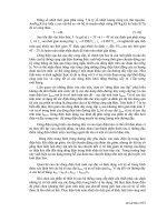
![[Điện Tử Học] Ngắn Mạch Hệ Thống - Pgs.Ts.Lê Kim Hùng phần 7 pps](https://media.store123doc.com/images/document/2014_07/13/medium_ycu1405243258.jpg)
![[Kinh Tế Học] Thị Trường Mục Tiêu - Ths.Nguyễn Quỳnh Chi, phần 7 ppsx](https://media.store123doc.com/images/document/2014_07/13/medium_fpk1405268418.jpg)
![[Cơ Học Chất Lỏng] Thủy Khí Kỹ Thuật Úng Dụng - Huỳnh Văn Hoàng phần 7 pps](https://media.store123doc.com/images/document/2014_07/13/medium_lcLTa4BgqC.jpg)
![[Công Trình Cao Tầng] Công Nghệ Ván Khuôn Trượt - Bùi Mạnh Hùng phần 7 pps](https://media.store123doc.com/images/document/2014_07/13/medium_kvz1405268448.jpg)