CRC.Press A Guide to MATLAB Object Oriented Programming May.2007 Episode 1 Part 4 docx

34 A Guide to MATLAB Object-Oriented Programming
Defining arrays as column vectors is convenient for concatenation and ultimately vectorization.
When we add support for object arrays, the vectorized code dealing with column arrays will have
an easier syntax. Proper concatenation of row arrays across an array of objects is possible, but it
usually requires a call to vertcat. It is also convenient to store N-dimensional arrays as columns.
In this case, use a reshape call to change the array into the desired shape. Finally, standardizing
around column vectors as the default internal format makes maintenance much easier. Unless you
have a good reason to the contrary, always store private arrays as columns.
You might also be wondering about the lowercase m at the beginning of each private member
variable. The m serves several purposes. Beginning each fieldname with lowercase m identifies the
variable as a member variable, and such identification is often helpful during code development.
The syntax serves as a cue in the same vein as the variable name this and the lowercase c added
to the beginning of the class name. It helps remind you that the variable belongs to an object and
is private. As with the other cues, adding an m is not required. If you discover that it is not useful,
leave it off.
3.2.2.2 cShape Public Interface
It is too early in our study of the MATLAB implementation to do anything fancy. In this chapter,
we will define a set of member functions capable of implementing the interface; however, keep in
mind that as we learn new techniques we will drop support for some of them. Presently we have
two techniques that we can exploit: a get and set pair and a switch based on the number of input
arguments obtained using nargin. To demonstrate both, we will implement the interface for size
and scale with get and set pairs and border color with an internal switch. Since the requirements
did not dictate names and formats, we will take the liberty to define them ourselves.
Object-oriented design advises a minimalist approach when creating the interface. Each acces-
sor or mutator exposes a little more of the class’ internal workings. If we expose too much of the
implementation or if we expose it in an awkward way, our future options are limited. Remember,
once advertised, a function is part of the interface forever. This locks you into supporting legacy
areas of the interface that might have been better left hidden. Being prudent and miserly when
defining the interface keeps our classes nimble.
Encapsulation along with a minimalist interface create a certain amount of tension between the
data required to support normal operation and the data required to support development tasks like

unit testing. A normal interface that exposes all hidden variables doesn’t quite follow the philosophy
of encapsulation; however, efficient testing sometimes mandates full exposure. For example, an
accessor that calculates its output based on some combination of private variables is much easier
to test if you can set private values and execute the member function. The problem here is that you
now have more than one type of client. Each type has a different agenda and consequently needs
a different interface. Indeed, this common situation is often included in books discussing object-
oriented design.
You don’t have to supply the entire public interface to every client. MATLAB has some very
convenient ways to accommodate different clients. You can include relatively simple switches
designed to turn certain features on and off. You can support different access syntax to reveal
concealed elements. There are others but the full list includes topics we haven’t yet discussed.
Later, when you refer back to the list, some of the items will make more sense. The list includes
the following:
• Selectively add special-purpose member functions for use by special-purpose clients by
using secondary class directories and manipulating the path. The possibility of multiple-
class directories was first described in §2.2.1.1. Technically, member functions in a
C911X_C003.fm Page 34 Friday, March 30, 2007 11:17 AM
Member Variables and Member Functions 35
secondary directory are part of the interface; however, their use is generally easier to
control compared to the functions in the general interface.
• Temporarily modify the constructor so that it enables built-in support for special-purpose
clients. For example, private logical values can easily guard debug displays. In another
example, store a function handle in a private variable and let special-purpose clients
reference a more capable function.
• Conceal certain variables by making their access or mutate syntax more difficult com-
pared to public variable syntax. This is actually a good option when you want to maintain
the general appearance of a simple interface yet still add advanced capability for sophis-
ticated clients. So-called concealed variables might not be advertised as belonging to the
public interface, but they need to be treated as public.
• Use private functions that don’t require an object but still operate with member variables.

Instead of passing an object, simplify the arguments by passing dot-referenced values.
The resulting code will be modular and allows functions to be tested separately from
the class.
• Allow a class to inherit a parent class that temporarily adds interface elements, or create
a child class that includes an alternate interface. An inheritance-based solution is often
difficult because, currently, MATLAB has no intrinsic support for protected visibility.
Most of these options result in challenging implementations. Serving two masters is inherently
difficult. As the examples become more challenging, some of these techniques will be discussed
further. We will not be able to develop a complete solution, but we will develop some of the options.
In the case of our simple example, there are not a lot of decisions to make regarding the
interface. The client’s view of the interface is functionally defined as follows:
shape = cShape;
shape_size = getSize(shape);
shape = setSize(shape, shape_size);
shape_scale = getScale(shape);
shape = setScale(shape, shape_scale);
shape_color = ColorRgb(shape);
shape = ColorRgb(shape, shape_color);
shape = reset(shape);
where
shape is an object of type cShape.
shape_size is the 2 × 1 numeric vector [horizontal_size; vertical_size]
with an initial value of [1; 1].
shape_scale is the 2 × 1 numeric vector [horizontal_scale;
vertical_scale] with an initial value of [1; 1].
shape_color is the 3 × 1 numeric vector [red; green; blue] with an initial value
of [0; 0; 1].
All of these functions will be implemented as public member functions. The first function is the
constructor. The constructor is one of the required elements, and we already understand what it
needs to contain. The other member functions are the topic of this chapter.

C911X_C003.fm Page 35 Friday, March 30, 2007 11:17 AM
36 A Guide to MATLAB Object-Oriented Programming
First, notice that every mutator includes the mutated object as an output. MATLAB always
uses a pass-by-value argument convention. The mutator must pass out the modified object and the
client must assign the modified object to a variable or all changes will be lost. The syntax is simply
a fact of programming under a pass-by-value convention. In many respects, the syntax used in
object-oriented MATLAB programming would benefit from the addition of a pass-by-reference
approach. The assignin function can be used to emulate a pass-by-reference calling syntax.
Before you attempt this technique, you should consider the warnings mentioned in Chapter 21.
Second, notice that the input argument lists include a cShape object as the first argument.
This is one of the hallmarks of a member function. The member function needs the object so that
it operates on the correct data, and MATLAB needs the object’s type so that it can locate the
appropriate class-specific member function. MATLAB still uses the search path; however, an object
in the input list triggers some additional priorities. Before we discuss the member function imple-
mentations, we need to take another brief side trip to examine this critical detail.
3.2.3 A SHORT SIDE TRIP TO EXAMINE FUNCTION SEARCH PRIORITY
MATLAB uses something called the search path to locate and execute functions. The search path
is simply an ordered list of directories, and any function you want to run must exist in one of the
search-path directories. Even though it does not show up in the ordered list, the present working
directory is also included in the search. Private directories are also absent from the list, but search
rules include them too. Of particular interest to us are the class directories. Class directories are
also absent from the list, but we already know that MATLAB readily locates the constructor.
MATLAB can also locate member functions. In most cases, you will not encounter problems with
the search. For those rare occasions when a problem comes up, it is good to understand the rules.
MATLAB documentation already includes a good description of the rules. For all the various
conditions, I will refer you to those documents. Here, the emphasis is on the object-oriented aspects
of the rules.
MATLAB always applies the same set of rules when it searches for a function. MATLAB can
locate all files on the search path that have the same name; however, it only executes the first file
that it finds. A determination of the first file can be made because locations are ordered according

to a priority. The location of the class constructor and other public member functions has a very
high priority. In order, from highest priority to lowest, the top few are summarized in the list below.
1. The function is defined as a subfunction in the caller’s m-file.
2. The function exists in the caller’s /private directory. There are two subtle exceptions
to this rule. First, the rule does not extend to /private/private directories. Instead,
functions that exist in a private function’s directory are located with a priority of 2. The
subtle nature of this rule can catch you if you are trying to call another class’ overloaded
function from within a private function of the same name.
3. The m-file is a constructor. That is, a class directory named /@function_name exists
and contains the m-file named function_name.m. A free function on the path with
the same name as a constructor will not be found before the constructor. In §2.2.1.1 we
discussed the possibility of spreading member functions across multiple class directories.
Like-named class directories are searched in the order that their parent directory appears
in the path.
4. When the input argument list contains an object, the object’s class directories are
searched. In those cases when more than one object appears among the input arguments,
only one type is selected and there is a procedure for determining which type. Under
typical conditions, the first argument’s type is used. Atypical conditions involve the use
of superiorto and inferiorto commands. These commands and their use are
described in §4.1.1. Inheritance also affects the search. The directories for the object’s
C911X_C003.fm Page 36 Friday, March 30, 2007 11:17 AM
Member Variables and Member Functions 37
most specific type are searched first. The search continues in the parent directories until
all parent levels have been exhausted. Inheritance from multiple parents uses type supe-
riority to decide which path to traverse.
5. An m-file for the function is located in the present working directory (i.e., pwd).
6. The function is a built-in MATLAB function.
7. The function is located elsewhere on the search path.
Items 3 and 4 are important in understanding how MATLAB treats objects, classes, and member
functions. Inherent in the search is the notion of type. This is a little odd because we typically

think of MATLAB variables as untyped. Once we accept typing, we note that locating an object’s
member functions is among the search path’s highest priorities. Except for a few subtle situations,
the member functions are usually located first.
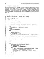
3.2.4 EXAMPLE CODE: ACCESSORS AND MUTATORS, ROUND 1
In §3.2.2 we expanded the requirements into a set of public member functions supported by a
private set of variables. This section implements conversion code. Accessors convert from the
private variable set to the return values expected. Mutators accept input values and convert these
values into a consistent, private, internal representation. As a demonstration of some of the power
behind the interface, the mutators in this implementation check for input assignment errors.
3.2.4.1 Constructor
Recall from §2.2.1.2 the constructor’s job: define the class structure and assign default values. The
constructor shown in Code Listing 4 meets all the requirements; it has the right name, it creates a
structure, and it calls class to convert the structure into an object. All we have to do is make
sure the file is stored as /@cShape/cShape.m. The structure is no longer being constructed
with a dummy field but rather includes the private variables identified in §3.2.2: mSize, mScale,
and mColorRgb. By setting the private variables to reasonable initial values, we avoid member
function errors and allow clients the luxury of omitting a lot of error-checking code.
3.2.4.2 Accessors
The class’ various interface functions were identified and defined in §3.2.2. Clients have read access
for every private variable. A get function from a get and set pair was defined as the interface to
both mSize and mScale. Accessors do not come any simpler compared to those shown in Code
Listing 5 and Code Listing 6 for getSize.m and getScale.m, respectively. The first line
defines the function. The second line uses dot-reference syntax to assign the private variable value
to the return argument. The simplicity of these functions relies on the operation of the constructor
Code Listing 4, A Very Simple Constructor
1 function this = cShape
2 this = struct(
3
‘mSize’, ones(2,1), % scaled [width height]’ of bounding
box

4
‘mScale’, ones(2,1), % [width height]’ scale factor
5 ‘mColorRgb’, [0 0 1]’ % [R G B]’ of border, default
is blue
6
);
7 this = class(this, ‘cShape’
);
C911X_C003.fm Page 37 Friday, March 30, 2007 11:17 AM
38 A Guide to MATLAB Object-Oriented Programming
and the mutators. For the cShape class, the constructor and the mutators must carefully control
what is assigned into the private variables.
The private variable mColorRgb also gets an accessor, but we will not implement its accessor
using a get function. Instead, the implementation combines both accessor and mutator into a single
function. The implementation is found in §3.2.4.4.
3.2.4.3 Mutators
Like the accessors, the mutators were identified and defined in §3.2.2. Clients have write access
for every private variable. A set function from a get and set pair was defined as the interface to
both mSize and mScale. Mutators rarely get any simpler compared to those shown in Code
Listing 7 and Code Listing 8 for setSize.m and setScale.m, respectively.
In Code Listing 7, line 1 defines the function. Line 2 sets the horizontal and vertical scale
factor to 1:1 whenever a new size is assigned. This behavior was not specified, but it seems to be
a reasonable thing to do. The alternate behavior would simply leave the scale factor with its current
value. Line 3 enters a switch based on the number of values passed via ShapeSize. Line 5
expands the size value to both directions when a scalar value is passed in. This behavior was not
specified, but most MATLAB functions seem to provide this sort of flexibility. Line 7 performs
the assignment when two values are passed in. These two values can occupy two elements of an
array of any dimension, and they will still be correctly assigned into mSize as a 2 × 1 column.
Again, this behavior was not specified, but such flexibility is generally expected. Finally, if any
number of values other than 1 or 2 is passed in, an error is thrown.

In most respects, Code Listing 8 is equivalent to Code Listing 7. Line 2 is different because it
calls the reset function. Since we are applying a new scale factor, we need to reset the shape
Code Listing 5, getSize.m Public Member Function
1 function ShapeSize = getSize(this)
2 ShapeSize = this.mSize;
Code Listing 6, getScale.m Public Member Function
1 function ShapeScale = getScale(this)
2 ShapeScale = this.mScale;
Code Listing 7, setSize.m Public Member Function
1 function this = setSize(this, ShapeSize)
2 this.mScale = ones(2,1); % reset scale to 1:1 when size
is set
3
switch length(ShapeSize(:))
4 case 1
5 this.mSize = [ShapeSize; ShapeSize];
6 case 2
7 this.mSize = ShapeSize(:); % ensure 2x1
8 otherwise
9
error('ShapeSize must be a scalar or length == 2');
10 end
C911X_C003.fm Page 38 Friday, March 30, 2007 11:17 AM
Member Variables and Member Functions 39
back to its original size before we can apply and store the new scale. The details for reset can
be found in §3.2.4.5. Line 11 resizes the shape by multiplying the reset size by the new scale value.
These two functions demonstrate the elegance of encapsulation by keeping mSize and mScale
in synch. The two variables are coupled so that whenever one changes, the other must also change.
Encapsulation enforces the use of the member functions, making it impossible for clients to change
one without changing the other. The coupled values always maintain their proper relationships.

3.2.4.4 Combining an Accessor and a Mutator
So far, we have not defined an accessor or mutator for mColorRgb. We could of course define a
get and set pair of functions, but we have already investigated that syntax. Instead, let’s look at a
syntax that combines the functionality of both accessor and mutator into a single member function.
The combined implementation is shown in Code Listing 9.
Code Listing 8, setScale.m Public Member Function
1 function this = setScale(this, ShapeScale)
2 this = reset(this); % back to original size (see Code
Listing 10)
3
switch length(ShapeScale(:))
4 case 1
5 this.mScale = [ShapeScale; ShapeScale];
6 case 2
7 this.mScale = ShapeScale(:); % ensure 2x1
8 otherwise
9
error('ShapeScale must be a scalar or length == 2');
10 end
11 this.mSize = this.mSize .* this.mScale; % apply new scale
Code Listing 9, ColorRgb.m Public Member Function
1 function return_val = ColorRgb(this, Color)
2 switch nargin % get or set depending on number of arguments
3
case 1
4 return_val = getColorRgb(this);
5 case 2
6 return_val = setColorRgb(this, Color);
7 end
8 otherwise

9 %
10 function ColorRgb = getColorRgb(this)
11 ColorRgb = this.mColorRgb;
12
13 %
14 function this = setColorRgb(this, Color)
15 if length(Color(:)) ~= 3
16
error('Color must be length == 3');
17 end
18 if any(Color(:) > 1) | any(Color(:) < 0)
19
error('all RGB Color values must be between 0 and 1');
20 end
21 this.mColorRgb = Color(:); % ensure 3x1
C911X_C003.fm Page 39 Friday, March 30, 2007 11:17 AM
40 A Guide to MATLAB Object-Oriented Programming
The switch in line 2 sorts out whether the member function is being called as an accessor
or mutator. If nargin equals one, the lone input must be a cShape object. The function is not
provided with an assignment value; therefore, the client must be requesting read access. Read
access calls the subfunction getColorRgb and simply returns the value stored in mColorRgb.
If nargin equals two, the function operates as a mutator. In the two-argument case, the object
and the assignment value are passed into the subfunction setColorRgb. Line 15 verifies the
number of color values, and line 18 verifies their values. If the values are okay, they are assigned
into the object as a 3 × 1 column. The modified object is passed back to the client.
The switch in line 2 doesn’t need an otherwise case because MATLAB will never allow a
member function other than the constructor to be called without an argument. Function-search rules
allow MATLAB to locate a function inside a class directory only when an argument’s type matches
the type of a known class. With no argument, MATLAB has no type to check. MATLAB might
find and execute a ColorRgb function, but it will not belong to any class.

3.2.4.5 Member Functions
With the current set of member functions, it is easy to get the wrong idea about accessors and
mutators. Accessors and mutators are not limited to simply returning or assigning values one-to-
one with private member variables. As we add capability to cShape, we will see that accessors
and mutators are more varied. Member functions can do anything a normal MATLAB function can
do because they are normal MATLAB functions. Just because they possess the special privilege of
reading and writing private variables does not preclude them from doing other things. This includes
calling member functions, calling general functions, graphing data, and accessing global data.
As an initial example, the expanded requirements stipulate a reset function. Unlike the other
member functions, neither the function name nor the argument list implies a direct connection to
a private variable. We know reset is a mutator because it passes the object back to the client.
As long as reset behaves properly, clients do not need to worry about the private changes that
take place. Behaving properly in the current context means resetting the shape’s scale to 1:1 and
adjusting the size back to the value assigned in the constructor or in setSize. The implementation
is provided in Code Listing 10.
Line 1 defines the function. The function is a mutator because the object, this, is passed in
and out. Line 2 loops over all objects in this. We could vectorize the code with calls to num2cell
and deal. Line 3 calculates the object’s size by dividing the current size by the current scale. This
calculation never needs to worry about a variable mismatch because the mutators work together in
ensuring that data are always stored in the proper format. A simple addition to setScale could
add protection from divide-by-zero warnings. Line 4 resets the scale back to 1:1.
3.2.5 STANDARDIZATION
The current implementation presents two equivalent implementation approaches that result in big
differences in client syntax. One method uses a pair of get and set functions, while the other
Code Listing 10, reset.m Public Member Function
1 function this = reset(this)
2 for k = 1:length(this(:))
3
this(k).mSize = this(k).mSize ./ this(k).mScale; % divide
by scale

4 this(k).mScale = ones(2,1); % reset scale to 1:1
5 end
C911X_C003.fm Page 40 Friday, March 30, 2007 11:17 AM
Member Variables and Member Functions 41
combines accessor and mutator capabilities into a single function. In my opinion, it is a bad idea
to follow this example and mix the use of both methods in the interface for a single class. It is
much better to choose one method and apply it consistently. In a similar vein, a library composed
of many classes is simply easier to use when all member functions use the same syntax. This
broadens the scope considerably because it typically means development teams should standardize
around a single method.
It seems reasonable to ask which approach is better. Unfortunately, there is no clear-cut winner.
The combined syntax is convenient because it results in fewer m-files overall. The combined syntax
also collects code associated with the same variable into the same source file. In my experience,
co-located accessor and mutator code is easier to maintain. On the other hand, get and set syntax
inherently describes the interface. If a variable has no associated set function, it means the variable
is not mutable, at least not directly. Identifying read-only versus read-write variables based on the
member function list is easy. The function name used by the combined syntax does not provide
this level of detail. In Chapter 8, when we will discuss a command-line feature called tab completion,
we will see how to get a complete list of public member functions. Finally, some clients prefer get
and set syntax.
Fortunately, MATLAB provides another alternative. Consider again our earlier attempt to
inspect the value shape.dummy. We tried this approach because the syntax is universally recog-
nized. It says there is a structure variable named shape and we think it has a field named dummy.
Using dot-reference notation is elegant, easy, and entrenched. What if MATLAB included a way
for objects to handle dot-reference notation? If such a feature exists, choosing get and set vs. a
combined syntax is a lot less urgent. MATLAB does indeed support this capability. We will discuss
dot-reference support in the next chapter. First, let’s take the current cShape class for a test drive.
3.3 THE TEST DRIVE
Our class now has the beginnings of an interface and we can use the interface to interact with
objects of the class. We need to construct some cShape objects and exercise the interface. We

need to both demonstrate the syntax and make sure objects behave according to the requirements.
The commands shown in Code Listing 11 provide a sample of cShape’s new capability.
Code Listing 11, Chapter 3 Test-Drive Command Listing
1
>> cd 'C:/oop_guide/chapter_3'
2
>> set(0, 'FormatSpacing', 'compact')
3
>> clear classes; clc;
4 >> shape = cShape;
5 >> shape = setSize(shape, [2 3]);
6 >> getSize(shape)'
7 ans =
8 2 3
9 >> shape = ColorRgb(shape, [1 0 1]);
10 >> ColorRgb(shape)'
11 ans =
12 1 0 1
13 >> getScale(shape)'
14 ans =
15 1 1
16 >> shape = setScale(shape, [2 4]);
17 >> getScale(shape)'
18 ans =
19 2 4
C911X_C003.fm Page 41 Friday, March 30, 2007 11:17 AM
42 A Guide to MATLAB Object-Oriented Programming
From the command results, we see that objects of the class behave as we expect. Lines 1–3
move us into the correct directory, configure the display format, and clear the workspace. Line 4
calls the cShape constructor. Line 5 assigns a size, and line 6 shows that the size was correctly

assigned.* Similarly, lines 9 and 10 mutate and access the shape’s color using the dual-purpose
function ColorRgb. Line 13 displays the default scale factor, and line 16 assigns a new scale.
Lines 17–22 show that directly mutating the scale indirectly mutates the size. Lines 23–26 show
that reset returns size back to its most recent setSize value. Finally, displaying the shape
results in the same cryptic message we saw in Chapter 2. In Chapter 5, we will replace this cryptic
output with an output tailored for the class.
3.4 SUMMARY
The primary topic in this chapter was encapsulation. Encapsulation is one of the three pillars of
object-oriented programming and as such carries a heavy load. Therefore, it is impossible to cover
every aspect in one chapter. This chapter did lay a solid foundation by including the most important
aspects. Primarily, encapsulation includes the idea of an interface, and an interface brings with it
a separation between so-called members and nonmembers. Membership has its privileges. For a
class, membership means unrestricted access to hidden or private variables and functions. Non-
members are restricted to public variables and functions.
Member functions are physically located inside a class directory. This allows MATLAB to find
them by checking a variable’s type. To do this, MATLAB follows the search path. We saw that
additional object-oriented search locations are one of the many consequences of encapsulation.
Now that we understand both path rules and encapsulation, locating the additional search directories
is a simple matter of applying the rules.
Member functions come in three flavors: constructor, accessor, and mutator. These three types
of member functions work in concert to provide object consistency. Each type serves a particular
role in the client-to-object interface. Constructors create the object’s private structure and assign
default values. Accessors provide read access, while mutators provide assignment capability. Encap-
sulation supports different connection options between the interface and the private variables. The
most straightforward connects private variables one-to-one with an interface function. The most
powerful completely separates the interface from the implementation. The most common uses a
combination of the two.
Even though the member functions in this chapter are basic, they reveal the potential power of
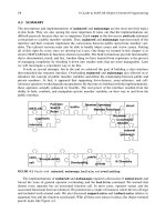
encapsulation. By adding these pieces, our object-oriented puzzle is off to a good start. Figure 3.1
shows us that we are missing pieces, but it also shows us that we are well on our way toward filling

out the frame.
20 >> getSize(shape)
21 ans =
22 4 12
23 >> shape = reset(shape);
24 >> getSize(shape)
25 ans =
26 2 3
27 >> shape
28 shape =
29 cShape object: 1-by-1
* The member variable mSize should not be confused with the MATLAB function size. They represent different things.
Now suppose we developed a combined accessor and mutator named Size. The potential for confusion is certainly high.
C911X_C003.fm Page 42 Friday, March 30, 2007 11:17 AM
Member Variables and Member Functions 43
3.5 INDEPENDENT INVESTIGATIONS
1. Modify setScale to protect other member functions from divide by zero errors.
2. Investigate path-search rules in action. Create functions with the same name, locate them
in various directories, and call them with various arguments. Place a function in a
/private directory in the class directory and see if MATLAB can find it. Try to get
MATLAB to find a function located in a /private/private directory. Inside each
function, you can use mfilename(‘fullpath’) to display the complete search
path. You can also use keyboard to prevent an infinite recursive loop.
3. Investigate more implementation alternatives. Instead of a series of get and set pairs
tailored for each member variable, can you design a general accessor named get.m and
a general mutator named set.m? (Hint: look at help for getfield and setfield.)
If your implementation relies on a large switch statement, can you use dynamic-field-
name syntax instead? Which implementation is more extendable and maintainable?
4. Try to enhance the interface. Most of your clients want to set the color using a string
like ‘red’ or ‘blue’. What do you do: eliminate the use of [r g b] values from the

interface spec? Write a new member function? Modify ColorRgb.m? (Hint: look at
help for ischar and isnumeric.) How does each choice influence quality measures?
5. Examine one benefit of encapsulation. Suppose you need to change the implementation
and store colors in HSV (hue–saturation–value) format but you can’t change the interface
in any way. What changes are required inside ColorRgb.m? (Hint: look at help for
rgb2hsv and hsv2rgb.) Do you need to change other member functions? Don’t forget
the constructor. You should be able to implement this change. Try it and see how well
you can do.
6. Examine another encapsulation option. Half your member functions need an RGB format,
and half need HSV. Clients always specify colors in terms of RGB. You have three
options: store the color using RGB format, store the color using HSV format, or store
both formats and rely on member functions to keep them synchronized. Which option
do you choose? Suppose you know the color is rarely changed and the conversion from
FIGURE 3.1 Puzzle with member variable, member function, and encapsulation.
@ Directory
Member Variables
Member Functions
struct
Encapsulation
class
call
Constructor
Mutator
Accessor
Function
Search
Rules
MATLAB
C911X_C003.fm Page 43 Friday, March 30, 2007 11:17 AM
44 A Guide to MATLAB Object-Oriented Programming

RGB to HSV is very expensive. Does this additional information push you toward a
different option? Without the benefit of encapsulation, keeping multiple copies of the
same data is risky business. Does encapsulation change the level of risk involved?
C911X_C003.fm Page 44 Friday, March 30, 2007 11:17 AM

45

4

Changing the Rules … in
Appearance Only

Near the end of the previous chapter, I alluded to the fact that MATLAB gives us a way to tailor
standard dot-reference syntax to suit the needs of our objects. In the eyes of our clients, dot-
reference tailoring makes an object look like a structure. This gives objects an enormous boost. If
objects look like structures, using objects rather than structures is completely transparent. Trans-
parency is a good thing because it gives us immediate access to a very powerful tool we can use
to protect the integrity of our code, encapsulation.
The good news is that MATLAB allows dot-reference tailoring. In this chapter, we will develop
a set of member functions that implement the tailoring in a way that allows objects to mimic
structures. We will take advantage of a pair of standard, but relatively unknown, functions,

sub-
sref.m

and

subsasgn.m

. The built-in versions operate on structures. Tailored versions, as long

as MATLAB can find them, operate on objects. From Chapter 3, we know MATLAB will find
them as long as they exist in the class directory as member functions. As tailored member functions,

subsref.m

and

subsasgn.m

are so critical to object-oriented programming that they share a
place beside the constructor in the group of eight.

4.1 A SPECIAL ACCESSOR AND A SPECIAL MUTATOR

The reason these very important functions are not well-known is that outside the realm of object-
oriented programming, they are almost never called by name. MATLAB classifies these functions
as operators in the same way it classifies symbols like

+

,

-

,

/

, and

~=

as operators. There are
many operators (see Table 4.1), but the distinguishing feature is syntax. When MATLAB encounters
an operator, it orders the arguments and converts the operator’s symbol into a function call. Unless
you understand what it means to be an operator, you might not realize what is going on behind
the scenes. Shortly we will specifically examine

subsref.m

and

subsasgn.m

operators. First,
let’s take a brief side trip to discuss operators and introduce a technique called operator overloading.

4.1.1 A S

HORT

S

IDE

T

RIP

TO

E

XAMINE

O

VERLOADING

Most of the symbols you can type from the keyboard have special meaning. The meanings behind

+

,

-

,

/

, and

~=

are clear. These special symbols are called operators. When MATLAB interprets
a line of code, it maps every operator to an m-file. Table 4.1 lists the mapping from symbol to m-
file. From the command line, you can display a similar list using

help ops

. If you look at the
list you see conversions like

+



⇒



plus.m

and

<=



⇒



le.m

. We can call these functions by name,
but we almost never do because operator syntax is a lot easier.

Stop for a minute and consider the implications. Every operator maps to an m-file, and the
execution of every m-file is determined based on the search path. That means we can redefine the
operation of any operator. All we have to do is create a new m-file with the same name as the
operator and put it in a directory with a higher search-path priority. For objects, we simply put the
tailored operator function in the class directory. Since MATLAB searches for member functions
before it searches for built-in functions, the tailored function has higher priority. Clients use normal
operator syntax, and MATLAB conveniently finds the appropriate function.

C911X_C004.fm Page 45 Friday, March 30, 2007 11:23 AM

46

A Guide to MATLAB Object-Oriented Programming

Object-oriented terminology calls this technique operator overloading, and every function in
Table 4.1 can be overloaded. When MATLAB encounters operator syntax, it collects variables into
argument lists and calls the operator’s function. Once you know the name of the operator’s function,
you can display the function’s help information to get a description of the arguments. For example,
the statement

c = a + b;

converts to the function equivalent

c = plus(a, b);

.
Operator overloading represents an important subset of general function overloading. General
function overloading allows a class to customize the operation of virtually any function by including
a tailored copy of the function in the class directory. Thus, any discussion of overloading involves

two functions, the function doing the overloading and the function being overloaded. Let’s refer
to the function doing the overloading as the tailored version and to the function being overloaded
as the original version.
With very few exceptions, MATLAB allows a class to overload any function. The original
function might exist as a built-in function or as a function on the path. If we jump ahead and
consider inheritance, the original function might also exist as a parent-class function. In short, once
a class overloads a function, the location of the original isn’t too important.

TABLE 4.1
Overloadable Operators

Operator Symbol m-file Name

a & b and.m
a:b colon.m
a’ ctranspose.m
a(end) end.m
a == b eq.m
a >= b ge.m
a > b gt.m
[a b] horzcat.m
a .\ b ldivide.m
a <= b le.m
loading object from .MAT file loadobj.m
a < b lt.m
a – b minus.m
a \ b mldivide.m
a ^ b mpower.m
a / b mrdivide.m
a * b mtimes.m

a ~= b ne.m
~a not.m
a | b or.m
a + b plus.m
a .^ b power.m
a ./ b rdivide.m
saving object to .MAT file. saveobj.m
a(k)=b, a{k}=b, or a.field=b subsasgn.m
x(a) subsindex.m
a(k), a{k}, and a.field subsref.m
a .* b times.m
a.’ transpose.m
-a uminus.m
+a uplus.m
[a; b] vertcat.m

C911X_C004.fm Page 46 Friday, March 30, 2007 11:23 AM

Changing the Rules … in Appearance Only

47

Given the ability to overload almost any function, you are also given the responsibility of doing
it wisely. Unfortunately, this is an area where experience is the best guide. There are few hard-and-
fast rules, but there are some things to consider. Original functions are generally well understood,
and overloading works best when the behavior of the tailored version can be inferred from the
behavior of the original. The argument syntax of an original function is also well-known, and the
tailored version should match the syntax very closely. This is particularly true for operator over-
loading because you can’t control the conversion from operator syntax to function call.
The implementation examples and the group of eight represent a good resource for examining

operator and function overloading. As we progress through the example code, you will be building
experience.

4.1.1.1 Superiorto and Inferiorto

In §3.2.3 the description of function-search rules conveniently assumed there was only one input
argument. Finding the correct function is a simple matter of including the argument’s class directory
in the search. Most functions require more than one input argument. With the prospect of more
than one type, we need to understand what MATLAB does to locate the correct function.
Some object-oriented languages select a function based on the combination of all input argu-
ments; however, MATLAB always uses one input argument. For functions with more than one
input, a priority scheme picks the argument with the highest priority. By default,

class

creates
all classes at the same priority level. After that, user-defined types can increase their relative priority
by calling

superiorto

and decrease it by calling

inferiorto

. Calls to these functions must
occur inside the constructor, and that means built-in types cannot change their priority. When one
argument clearly has the highest priority, its type is used in the search. When one argument is not
the clear winner, argument order is used as a tiebreaker. In this case, the type of the first tied
argument in the argument list is used.

If all arguments have the same type, MATLAB uses the type of the very first argument. This
is convenient for a number of reasons. First, a single priority eliminates errors that occur due to
unanticipated argument combinations. If you set up a complicated priority tree, it is easy to find
yourself in an unexpected function call. Second, a single priority makes it easy to understand which
class directory will be selected. It will always correspond to the first argument’s type. Finally, with
a single priority you never need to search the argument list to find

this

. The active object is
always passed in the first position.
Classes that overload operators usually need to increase their priority relative to built-in types.*
This is particularly true for commutative operators like

+

because the object can be passed using
either argument. Relying on default priority will result in an error about half the time. When the
object shows up on the left side of the operator, the tailored version executes and all is well;
however, when the object shows up on the right-hand side, MATLAB will call the built-in version
and the built-in version does not know what to do with an object. For example,

obj+1

is converted
into the function call expressed as

plus(obj, 1)

. Here the

plus

function associated with

obj

correctly executes. Switch the argument order to

1+obj

and the conversion becomes

plus(1,
obj)

. If

1

and

obj

have the same priority, the built-in

plus

will be called and the result will be
an error. To remedy this situation, the constructor needs to include the command

superi-
orto(‘double’)

.
Other than superiority over built-in types, the software design ultimately determines the com-
plexity of the priority tree and thus represents a barrier to implementing some object-oriented
designs in MATLAB. The barrier is not impossible to cross but does limit extendibility in some
designs. When one of the design constraints is to limit the number of priority levels, the result is

* In version 7.1 (R14), this is no longer true. User-defined types are superior to the built-in types. Relative argument
priority still applies to operations using user-defined types.

C911X_C004.fm Page 47 Friday, March 30, 2007 11:23 AM

48

A Guide to MATLAB Object-Oriented Programming

a better implementation. For designs with a small number of classes and a reasonably flat structure,
the risk is low. By the time your designs approach that level of complexity, you will be well
equipped to consider priority as a constraint.

4.1.1.2 The Built-In Function

More often than you might imagine, you need to call the original version of a function from inside
the tailored version. For example, suppose you design a class interface that makes objects of the
class look like a simple one-dimensional array of doubles. To implement the interface, you need
to overload

length

,

ndims

,

numel

, and

size

. Depending on the private variable organization,
all of these tailored functions might need to call the built-in version of

size

. We can’t simply
write

size(this)

because path rules insist on running the tailored version.
The

builtin

function solves this problem. The argument syntax for

builtin

uses the same
syntax as

feval

. The name of the function is the first input argument, and the remaining inputs
are passed into the function named in argument one. The output arguments are declared the same
as if the function was being called directly. The prototype for this function is

[y1, …, yn] = builtin(‘function_name’, x1, …, xn);

The availability of

builtin

solves one problem but creates another. Clients can use

builtin

to circumvent the interface and violate the integrity of the encapsulation. Unfortunately, we can’t
stop them. All we can reasonably do is dissuade them from using

builtin

and periodically search
for its use.

4.1.2 O

VERLOADING



THE

O

PERATORS



SUBSREF



AND



SUBSASGN

It may come as a surprise to realize that

.

,

()

, and

{}

are operators. If you scan Table 4.1, you
will see that dot-reference, array-reference, and cell-reference syntax map to

subsref.m

and

subsasgn.m

. Thus, using one of these index operators on an object tells MATLAB to call that
object’s version of

subsref or subsasgn. It is up to us to include the appropriate class-specific
commands in the body of each. These functions are the most important operator functions we will
encounter because they allow us to create an easy-to-use interface. This will become clear as we
progress through the examples. The accessor is subsref, and the mutator is subsasgn. Each
function can determine which operator triggered the call because MATLAB passes a specially
formatted version of the operator along with the other arguments.
In Chapter 3 the only member function tools at our disposal consisted of a pair of get and
set functions for each public member variable. With operator overloading and the availability of
subsref and subsasgn, get and set syntax can be easily replaced by dot-reference syntax.
Doing so makes the interface a lot more convenient because it looks like something very familiar,
a structure.
In the test drive for Chapter 3, we wrote,

shape_size = getSize(shape);
shape = setSize(shape, [10; 20]);
In the test drive for this chapter, we will be able to write,
shape_size = shape.size;
shape.size = [10; 20];
Compared to the other operators, more code is required to implement tailored versions of
subsref and subsasgn. For the most part the additional code results from the fact that each
C911X_C004.fm Page 48 Friday, March 30, 2007 11:23 AM
Changing the Rules … in Appearance Only 49
function must handle three operators. Using a switch statement to select the appropriate case is an
easy approach. First, let’s look at the function syntax.
The function definitions for subsref.m and subsasgn.m can be written as
function varargout = subsref(this, index)
function this = subsasgn(this, index, varargin)
In both cases the first argument is the active object this. Since MATLAB passes this as the
first argument, these operator overloads don’t require calls superiorto or inferiorto.
The second argument, index, is a specially packaged version of the operator and indices. In
addition to supporting three different operators, index also supports multiple index levels. Another
obscure function, substruct, can be used to create the special packaging, and because of this,
the index format is also called substruct. All substruct indices are stored as a structure
array with two fields:
index(k).type
index(k).subs
Each index level represented by index(k) contains a type field and a subs field. The type
field is a string containing one of three string values: ‘.’, (), or {}. These three string values
respectively represent a dot-reference, array-reference, and cell-reference operation. When MAT-
LAB converts operator syntax into an index, only certain combinations of operators and levels
are converted.
When the type field is ‘.’, the subs field will contain a character string that names the
desired public member variable. When the type field is () or {}, the subs field will contain a

cell array. Each cell index holds the index values for one dimension. The values in
index(k).subs{1} are used to select values in the first dimension, values in
index(k).subs{2} the second dimension, and so on. With one exception, the index values
will be packaged as a fully expanded array. The lone exception occurs when the specified index
was ‘:’. In that case, the index value is equal to ‘:’. Fortunately, when the type field is () or
{}, we don’t need to manage the contents of the subs field on our own. Instead, we can coerce
MATLAB into performing all of the low-level work. We still have to process ‘.’ and the public
variable names; but, since there is only one format, that is the easy case.
The standard set of allowed values for type is well defined and small, making a switch
statement ideal for implementation.* The
switch skeleton is shown in Code Listing 12. This
Code Listing 12, Skeleton Switch Statement for subsref and subsasgn
1 switch index (1).type
2 case '.'
3 % code to deal with the fieldname in index(1).subs
4 case '()'
5 % code to deal with an array of index values
6 case '{}'
7 % code to deal with cell array of index values
8 otherwise
9 error(['Unexpected index.type of ' index(1).type]);
10 end
* It is possible to pass nonstandard operators into subsref and subsasgn but not via automatic operator conversion.
A manually created substruct index can include an arbitrary type string, and this index can be passed into substruct
or subsasgn if the functions are called by name. Adding new access categories might seem bizarre, but might actually
be useful under the right set of circumstances. Nonstandard indices are not supported by the built-in versions of subsref
and subsasgn, and they are not supported by Class Wizard.
C911X_C004.fm Page 49 Friday, March 30, 2007 11:23 AM
50 A Guide to MATLAB Object-Oriented Programming
skeleton is used inside both subsref and subsasgn. Before filling in code for each case, I need

to outline an approach for discussing the boxes shown in Figure 4.1. One organization discusses
all cases of subsref before moving on to all cases of subsasgn. The alternate organization
discusses one operator case with respect to both access and mutation before moving on to the
next. As you might expect, there is a lot of overlap between these alternate paths. The discussion
seems to work better when access and mutation for a single case are covered together.
4.1.2.1 Dot-Reference Indexing
The dot-reference operator looks something like the following:
b = a.field;
a.field = b;
When MATLAB encounters these statements, it converts them into the equivalent function calls
given respectively by
b = subsref(a, substruct(‘.’, ‘field’));
a = subsasgn(a, substruct(‘.’, ‘field’), b);
The two representations are exactly equivalent. You will probably agree that dot-reference operator
syntax is much easier to read at a glance compared to the functional form. The functional form
gives us some important details to use during the implementation of subsref and subsasgn.
With either conversion, the index variable passed into both subsref and subsasgn is
composed using substruct(‘.’, ‘field’). The type field is of course ‘.’ and the
element name is represented here by the subs field value ‘field’. The substruct argument
is a structure, and the MATLAB display looks like the following:
If all we want to do is provide a 1:1 mapping between public and private member variables,
the ‘.’ case of subsref would include just one line*:
FIGURE 4.1 Access operator organizational chart.
1 >> index = substruct('.', 'field')
2 index =
3 type: '.'
4 subs: 'field'
* Dynamic fieldname indexing works for versions 7.0 and later. In some earlier versions, dynamic field syntax did not
always work from inside a member function. If dynamic fieldname syntax generates an error, revert to the use of properly
formatted calls to getfield or setfield.

Access Operators
subsref subsasgn
dot-access
array-access
cell-access
dot-access
array-access
cell-access
C911X_C004.fm Page 50 Friday, March 30, 2007 11:23 AM
Changing the Rules … in Appearance Only 51
varargout = {this.(index(1).subs)};
Similarly, the ‘.’ case of subsasgn would include the following line:
this.(index(1).subs) = varargin{1};
The one-line 1:1 mapping code works well as an introduction but is too simplistic for most classes.
For example, the one-line solution does not support multiple indexing levels, and it doesn’t support
argument checking. Even worse, the one-line solution maps every private member variable as
public. It is easy to address each of these deficiencies by adding more code and checking more
cases. By the end of this chapter, we will have a good working knowledge of subsref and
subsasgn, but we will not yet arrive at their final implementation. The final implementation relies
on first developing some of the other group-of-eight members.
4.1.2.2 subsref Dot-Reference, Attempt 1
One potential solution to the subsref challenge is shown in Code Listing 13. This solution is
similar to the solution outlined in the MATLAB manuals and is more versatile than the previous
one-liner. This approach might be okay for simple classes, but for classes that are more complicated
it needs improvement. The biggest downfall of the implementation in Code Listing 13 is the coupling
between the dot-reference name and private variable names. It also doesn’t take care of multiple
index levels and is not as modular as we might like. Such complaints are easily remedied. It just
takes a little more work to push it over the top.
Line 1 references the operator’s type. For dot-reference the type string is ‘.’ and execution
enters the case on line 2. Line 3 references the name included in the dot-reference index. This

name, specified by the client, is part of the public interface. That is an important point that bears
repeating. The string contained in index(1).subs is a public name. The situation in this code
Code Listing 13, By-the-Book Approach to subref’s Dot-Reference Case
1 switch index(1).type
2
case '.'
3
switch index(1).subs
4
case 'mSize'
5
varargout = {this.mSize};
6
case 'mScale'
7
varargout = {this.mScale};
8
case 'mColorRgb'
9 varargout = {this.mColorRgb};
10 otherwise
11 error(['??? Reference to non-existent field '
12 index(1).subs '.']);
13 end
14 case '()'
15 % code to deal with cell array of index values
16 case '{}'
17 % code to deal with cell array of index values
18 otherwise
19 error(['??? Unexpected index.type of ' index(1).type]);
20 end

C911X_C004.fm Page 51 Friday, March 30, 2007 11:23 AM
52 A Guide to MATLAB Object-Oriented Programming
example can be very confusing because the client’s interface and the private member variables
share the same name. Lines 4, 6, and 8 assign the private member variable with the same dot-
reference name into the output variable, varargout. We already know that object-oriented rules
prohibit clients from directly accessing private variables, but the contents of this version of sub-
sref seem like an attempt to get around the restriction. The source of the confusion comes from
making the public dot-reference names identical to the private variable names. The client doesn’t
gain direct access to each private member variable but the names make it seem so. The specific
cell-array assignment syntax in lines 5, 7, and 9 supports later extensions where this will exist
as an array of structures. Finally, line 11 throws an error if the client asks for a dot-reference name
not included in the list.
The subsref syntax is different compared to the get and set syntax from Chapter 3. Clients
usually prefer subsref syntax because it is identical to accessing a structure. In Chapter 3, the
only interface tool in our member function toolbox was get and set. With the addition of
subsref, we can now define a friendly interface. In doing so we will deprecate some of Chapter
3’s interface syntax.
4.1.2.3 A New Interface Definition
The initial interface syntax was defined in §3.2.2.2. Here we are going to make a couple of changes
that both take advantage of dot-reference syntax and allow the investigation of specific implemen-
tation issues. The client’s new view of the interface is defined as
shape = cShape;
shape_size = shape.Size;
shape.Size = shape_size;
shape = shape_scale * shape;
shape = shape * shape_scale;
shape_color = shape.ColorRgb;
shape.ColorRgb = shape_color;
shape = reset(shape);
where

shape is an object of type cShape.
shape_size is the 2 × 1 numeric vector [horizontal_size; vertical_size] with an initial
value of [1; 1].
shape_scale is the 2 × 1 numeric vector [horizontal_scale; vertical_scale] with an initial
value of [1; 1].
shape_color is the 3 × 1 numeric vector [red; green; blue] with an initial value of [0; 0; 1].
Notice that the only member functions implied by syntax are the constructor, cShape.m, and
reset. The functions getSize, setSize, and ColorRgb have been completely replaced by
subsref, subsasgn, and dot-reference syntax. Also, notice the abstraction of the client’s use
of a scale factor into multiplication and reset.
C911X_C004.fm Page 52 Friday, March 30, 2007 11:23 AM
Changing the Rules … in Appearance Only 53
4.1.2.4 subsref Dot-Reference, Attempt 2: Separating Public and
Private Variables
From the by-the-book approach in Code Listing 13, it would be easy to get the idea that objects
are just encapsulated structures and that subsref and subsasgn simply avoid a collection of
get and set functions. Nothing could be further from the truth. The real purpose of subsref
and subsasgn is to support encapsulation by producing an easy-to-use interface.
Let’s formalize some terminology that will simplify the discussions. To the client, values
associated with subsref’s dot-reference names are not hidden. Furthermore, dot-reference
syntax makes these values appear to be variables rather than functions. Based on appearances, we
will refer to the collection of dot-reference names as public member variables. This will differentiate
them from the fields in the private structure, that is, the private member variables. Even in Code
Listing 13, where public member variables and private member variables shared the same names,
clients could not directly access private variables. Cases inside subsref guard against direct
access.
As we will soon see, subsasgn also uses a switch on the dot-reference name and cases inside
subsasgn guard against direct mutation. The fact that MATLAB uses one function for access,
subsref, and a different function for mutation, subsasgn, gives us added flexibility. At our
option, we can include a public variable name in the switch of subsref, subsasgn, or both. If

the public variable name is included in subsref, the variable is readable. If the public variable
name is included in subsasgn, the public member variable is writable. A public variable is both
readable and writable when the name is included in both subsref and subsasgn. Independently
controlled read and write permissions also differentiate object-oriented programming from most
procedural programming. A complete interface specification should include the restrictions read-
only and write-only as appropriate, and these restrictions should be included in the implementations
of subsref and subsasgn.
Use different names to reinforce the idea that private member variables are separate from public
member variables. This is where the lowercase ‘m’ convention is useful. In one-to-one public-to-
private associations, the ‘m’ makes the code more obvious. The variable with a leading ‘m’ is
private, and the one without is public. There is a second part to the ‘m’ convention. If private
variables are named using the ‘m’ convention, no public variable should include a leading ‘m’.
For coding standards that only allow lowercase characters in variable names, expand the convention
from ‘m’ to ‘m_’ to avoid private names beginning with ‘mm’.
The subsref switch in Code Listing 14 implements the replacement. The difference from
the by-the-book approach occurs in lines 4 and 6, where the ‘m’ has been removed from the case
strings. The mScale case has also been removed. Now, dot-reference names match the new
interface definition from §4.1.2.3. Most variables in this example are still one-to-one, public-to-
private. Let’s remedy that situation next.
4.1.2.5 subsref Dot-Reference, Attempt 3: Beyond One-to-One,
Public-to-Private
For an example of a general public variable implementation, let’s change the internal color format.
One of the exercises at the end of Chapter 3 asked you to consider this exact change. Instead of
storing red-green-blue (RGB) values, we want to change the class implementation to store hue-
saturation values (HSV). For this change, we are not allowed to change the interface defined in
§4.1.2.3. According to the interface, the public variables use RGB values and the implementation
change must not cause errors in client code. To help in this change, MATLAB provides two
conversion functions, hsv2rgb and rgb2hsv. These functions allow us to convert between RGB
and HSV color representations.
C911X_C004.fm Page 53 Friday, March 30, 2007 11:23 AM