Data Analysis Machine Learning and Applications Episode 2 Part 1 pot

272 Daniel Meyer-Delius et al.
Fig. 2. passing maneuver and corresponding HMM.
an HMM that describes this sequences could have three states, one for each step of
the maneuver: q
0
= behind(R,R

), q
1
= left(R,R

),andq
2
= in_front_of(R,R

).
The transition model of this HMM is depicted in Figure 2. It defines the allowed
transitions between the states. Observe how the HMM specifies that when in the
second state (q
1
), that is, when the passing car is left of the reference car, it can
only remain left (q
1
) or move in front of the reference car (q
2
). It is not allowed to
move behind it again (q
0
). Such a sequence would not be a valid passing situation
according to our description.
A situation HMM consists of a tuple O =(

Q ,A,S), where Q = {q
0
, ,q
N
} rep-
resents a finite set of N states, which are in turn abstract states as described in the
previous section, A = {a
ij
} is the state transition matrix where each entry a
ij
repre-
sents the probability of a transition from state q
i
to state q
j
, and S = {S
i
}is the initial
state distribution, where S
i
represents the probability of state q
i
being the initial state.
Additionally, just as for the DBNs, there is also an observation model. In our case,
this observation model is the same for every situation HMM, and will be described
in detail in Section 4.1.
4 Recognizing situations
The idea behind our approach to situation recognition is to instantiate at each time
step new candidate situation HMMs and to track these over time. A situation HMM
can be instantiated if it assigns a positive probability to the current state of the sys-

tem. Thus, at each time step t, the algorithm keeps track of a set of active situation
hypotheses, based on a sequence of relational descriptions.
The general algorithm for situation recognition and tracking is as follows. At
every time step t,
1. Estimate the current state of the system x
t
(see Section 2).
2. Generate relational representation o
t
from x
t
: From the estimated state of the
system x
t
, a conjunction o
t
of grounded relational atoms with an associated prob-
ability is generated (see next section).
3. Update all instantiated situation HMMs according to o
t
: Bayes filtering is used
to update the internal state of the instantiated situation HMMs.
Probabilistic Relational Modeling of Situations 273
4. Instantiate all non-redundant situation HMMs consistent with o
t
: Based on o
t
,all
situation HMMs are grounded, that is, the variables in the abstract states of the
HMM are replaced by the constant terms present in o

t
. If a grounded HMM as-
signs a non-zero probability to the current relational description o
t
, the situation
HMM can be instantiated. However, we must first check that no other situation
of the same type and with the same grounding has an overlapping internal state.
If this is the case, we keep the oldest instance since it provides a more accurate
explanation for the observed sequence.
4.1 Representing uncertainty at the relational level
At each time step t, our algorithm estimates the state x
t
of the system. The estimated
state is usually represented through a probability distribution which assigns a proba-
bility to each possible hypothesis about the true state. In order to be able to use the
situation HMMs to recognize situation instances, we need to represent the estimated
state of the system as a grounded abstract state using relational logic.
To convert the uncertainties related to the estimated state x
t
into appropriate un-
certainties at the relational level, we assign to each relation the probability mass
associated to the interval of the state space that it represents. The resulting distribu-
tion is thus a histogram that assigns to each relation a single cumulative probability.
Such a histogram can be thought of as a piecewise constant approximation of the
continuous density. The relational description o
t
of the estimated state of the system
x
t
at time t is then a grounded abstract state where each relation has an associated

probability.
The probability P(o
t
|q
i
) of observing o
t
while being in a grounded abstract state
q
i
is computed as the product of the matching terms in o
t
and q
i
. In this way, the
observation probabilities needed to estimate the internal state of the situation HMMs
and the likelihood of a given sequence of observations O
1:t
=(o
1
, ,o
t
) can be
computed.
4.2 Situation model selection using Bayes factors
The algorithm for recognizing situations keeps track of a set of active situation hy-
pothesis at each time step t. We propose to decide between models at a given time t
using Bayes factors for comparing two competing situation HMMs that explain the
given observation sequence. Bayes factors (Kass and Raftery (1995)) provide a way
of evaluating evidence in favor of a probabilistic model as opposed to another one.

The Bayes factor B
1,2
for two competing models O
1
and O
2
is computed as
B
12
=
P(O
1
|O
t
1
:t
1
+n
1
)
P(O
2
|O
t
2
:t
2
+n
2
)

=
P(O
t
1
:t
1
+n
1
|O
1
)P(O
1
)
P(O
t
2
:t
2
+n
2
|O
2
)P(O
2
)
, (1)
that is, the ratio between the likelihood of the models being compared given the data.
The Bayes factor can be interpreted as evidence provided by the data in favor of a
model as opposed to another one (Jeffreys (1961)).
274 Daniel Meyer-Delius et al.

In order to use the Bayes factor as evaluation criterion, the observation sequence
O
t:t+n
which the models in Equation 1 are conditioned on, must be the same for the
two models being compared. This is, however, not always the case, since situation
can be instantiated at any point in time. To solve this problem we propose a solution
used for sequence alignment in bio-informatics (Durbin et al. (1998)) and extend the
situation model using a separate world model to account for the missing part of the
observation sequence. This world model in our case is defined analogously to the
bigram models that are learn from the corpora in the field of natural language pro-
cessing (Manning and Schütze (1999)). By using the extended situation model, we
can use Bayes factors to evaluate two situation models even if they where instantiated
at different points in time.
5 Evaluation
Our framework was implemented and tested in a traffic scenario using a simulated
3D environment. TORCS - The Open Racing Car Simulator (Espié and Guionneau)
was used as simulation environment. The scenario consisted of several autonomous
vehicles with simple driving behaviors and one reference vehicle controlled by a
human operator. Random noise was added to the pose of the vehicles to simulate un-
certainty at the state estimation level. The goal of the experiments is to demonstrate
that our framework can be used to model and successfully recognize different sit-
uations in dynamic multi-agent environments. Concretely, three different situations
relative to a reference car where considered:
1. The passing situation corresponds to the reference car being passed by another
car. The passing car approaches the reference car from behind, it passes it on the
left, and finally ends up in front of it.
2. The aborted passing situation is similar to the passing situation, but the reference
car is never fully overtaken. The passing car approaches the reference car from
behind, it slows down before being abeam, and ends up behind it again.
3. The follow situation corresponds to the reference car being followed from behind

by another car at a short distance and at the same velocity.
The structure and parameters of the corresponding situation HMMs where defined
manually. The relations considered for these experiments where defined over the
relative distance, position, and velocity of the cars.
Figure 3 (left) plots the likelihood of an observation sequence corresponding to
a passing maneuver. During this maneuver, the passing car approaches the reference
car from behind. Once at close distance, it maintains the distance for a couple of
seconds. It then accelerates and passes the reference car on the left to finally end up
in front of it. It can be observed in the figure how the algorithm correctly instan-
tiated the different situation HMMs and tracked the different instances during the
execution of the maneuver. For example, the passing and aborted passing situations
where instantiated simultaneously from the start, since both situation HMMs initially
Probabilistic Relational Modeling of Situations 275
-1600
-1400
-1200
-1000
-800
-600
-400
-200
0
5 10 15 20 25 30
log likelihood
time (s)
passing
aborted passing
follow
-200
-100

0
100
200
300
400
500
600
4 6 8 10 12 14 16 18 20 22
bayes factor
time (s)
passing vs. follow
Fig. 3. (Left) Likelihood of the observation sequence for a passing maneuver according to
the different situation models, and (right) Bayes factor in favor of the passing situation model
against the other situation models.
describe the same sequence of observations. The follow situation HMM was instanti-
ated, as expected, at the point where both cars where close enough and their relative
velocity was almost zero. Observe too that at this point, the likelihood according to
the passing and aborted passing situation HMMs starts to decrease rapidly, since
these two models do not expect both cars to drive at the same speed. As the passing
vehicle starts changing to the left lane, the HMM for the follow situation stops pro-
viding an explanation for the observation sequence and, accordingly, the likelihood
starts to decrease rapidly until it becomes almost zero. At this point the instance of
the situation is not tracked anymore and is removed from the active situation set. This
happens since the follow situation HMM does not expect the vehicle to speed up and
change lanes.
The Bayes factor in favor of the passing situation model compared against the
follow situation model is depicted in Figure 3 (right). A positive Bayes factor value
indicates that there is evidence in favor of the passing situation model. Observe that
up to the point where the follow situation is actually instantiated the Bayes factor
keeps increasing rapidly. At the time where both cars are equally fast, the evidence

in favor of the passing situation model starts decreasing until it becomes negative. At
this point there is evidence against the passing situation model, that is, there is evi-
dence in favor of the follow situation. Finally, as the passing vehicle starts changing
to the left lane the evidence in favor of the passing situation model starts increas-
ing again. Figure 3 (right) shows how Bayes factors can be used to make decisions
between competing situation models.
6 Conclusions and further work
We presented a general framework for modeling and recognizing situations. Our ap-
proach uses a relational description of the state space and hidden Markov models to
represent situations. An algorithm was presented to recognize and track situations
in an online fashion. The Bayes factor was proposed as evaluation criterion between
276 Daniel Meyer-Delius et al.
two competing models. Using our framework, many meaningful situations can be
modeled. Experiments demonstrate that our framework is capable of tracking multi-
ple situation hypotheses in a dynamic multi-agent environment.
References
ANDERSON, C. R., DOMINGOS, P. and WELD, D. A. (2002): Relational Markov models
and their application to adaptive web navigation. Proc. of the International Conference
on Knowledge Discovery and Data Mining (KDD).
COCORA, A., KERSTING, K., PLAGEMANN, C. and BURGARD, W. and DE RAEDT,
L. (2006): Learning Relational Navigation Policies. Proc. of the IEEE/RSJ International
Conference on Intelligent Robots and Systems (IROS).
COLLETT, T., MACDONALD, B. and GERKEY, B. (2005): Player 2.0: Toward a Practi-
cal Robot Programming Framework. In: Proceedings of the Australasian Conference on
Robotics and Automation (ACRA 2005).
DEAN, T. and KANAZAWA, K. (1989): A Model for Reasoning about Persistence and Cau-
sation. Computational Intelligence, 5(3):142-150.
DURBIN, R., EDDY, S., KROGH, A. and MITCHISON, G. (1998):Biological Sequence Anal-
ysis. Cambridge University Press.
FERN, A. and GIVAN, R. (2004): Relational sequential inference with reliable observations.

Proc. of the International Conference on Machine Learning.
JEFFREYS, H. (1961): Theory of Probability (3rd ed.). Oxford University Press.
KASS, R. and RAFTERY, E. (1995): Bayes Factors. Journal of the American Statistical As-
sociation, 90(430):773-795.
KERSTING, K., DE RAEDT, L. and RAIKO, T. (2006): Logical Hidden Markov Models.
Journal of Artificial Intelligence Research.
MANNING, C.D. and SCHÜTZE, H. (1999): Foundations of Statistical Natural Language
Processing. The MIT Press.
RABINER, L. (1989): A tutorial on hidden Markov models and selected applications in speech
recognition. Proceedings of the IEEE, 77(2):257–286.
ESPIÉ, E. and GUIONNEAU, C. TORCS - The Open Racing Car Simulator.

Applying the Q
n
Estimator Online
Robin Nunkesser
1
, Karen Schettlinger
2
and Roland Fried
2
1
Department of Computer Science, Univ. Dortmund, 44221 Dortmund, Germany

2
Department of Statistics, Univ. Dortmund, 44221 Dortmund, Germany
{schettlinger,fried}@statistik.uni-dortmund.de
Abstract. Reliable automatic methods are needed for statistical online monitoring of noisy
time series. Application of a robust scale estimator allows to use adaptive thresholds for the
detection of outliers and level shifts. We propose a fast update algorithm for the Q

n
estimator
and show by simulations that it leads to more powerful tests than other highly robust scale
estimators.
1 Introduction
Reliable online analysis of high frequency time series is an important requirement
for real-time decision support. For example, automatic alarm systems currently used
in intensive care produce a high rate of false alarms due to measurement artifacts,
patient movements, or transient fluctuations around the chosen alarm limit. Prepro-
cessing the data by extracting the underlying level (the signal) and variability of the
monitored physiological time series, such as heart rate or blood pressure can improve
the false alarm rate. Additionally, it is necessary to detect relevant changes in the ex-
tracted signal since they might point at serious changes in the patient’s condition.
The high number of artifacts observed in many time series requires the applica-
tion of robust methods which are able to withstand some largely deviating values.
However, many robust methods are computationally too demanding for real time
application if efficient algorithms are not available.
Gather and Fried (2003) recommend Rousseeuw and Croux’s (1993) Q
n
estima-
tor to measure the variability of the noise in robust signal extraction. The Q
n
pos-
sesses a breakdown point of 50%, i.e. it can resist up to almost 50% large outliers
without becoming extremely biased. Additionally, its Gaussian efficiency is 82% in
large samples, which is much higher than that of other robust scale estimators: for ex-
ample, the asymptotic efficiency of the median absolute deviation about the median
(MAD) is only 36%. However, in an online application to moving time windows the
MAD can be updated in
O(logn) time (Bernholt et al. (2006)), while the fastest algo-

rithm known so far for the Q
n
needs O(nlogn) time (Croux and Rousseeuw (1992)),
where n is the width of the time window.
278 Robin Nunkesser, Karen Schettlinger and Roland Fried
In this paper, we construct an update algorithm for the Q
n
estimator which, in
practice, is substantially faster than the offline algorithm and implies an advantage
for online application. The algorithm is easy to implement and can also be used
to compute the Hodges-Lehmann location estimator (HL) online. Additionally, we
show by simulation that the Q
n
leads to resistant rules for shift detection which have
higher power than rules using other highly robust scale estimators. This better power
can be explained by the well-known high efficiency of the Q
n
for estimation of the
variability.
Section 2 presents the update algorithm for the Q
n
. Section 3 describes a com-
parative study of rules for level shift detection which apply a robust scale estimator
for fixing the thresholds. Section 4 draws some conclusions.
2 An update algorithm for the Q
n
and the HL estimator
For data x
1
, ,x

n
, x
i
∈ R and k =

n/2+1
2

, a denoting the largest integer not
larger than a,theQ
n
scale estimator is defined as
ˆ
V
(Q)
= c
(Q)
n

|x
i
−x
j
|,1 ≤i < j ≤n

(k)
,
corresponding to approximately the first quartile of all pairwise differences. Here,
c
(Q)

n
denotes a finite sample correction factor for achieving unbiasedness for the
estimation of the standard deviation V at Gaussian samples of size n. For online
analysis of a time series x
1
, ,x
N
, we can apply the Q
n
to a moving time win-
dow x
t−n+1
, ,x
t
of width n < N, always adding the incoming observation x
t+1
and
deleting the oldest observation x
t−n+1
when moving the time window from t to t +1.
Addition of x
t+1
and deletion of x
t−n+1
is called an update in the following.
It is possible to compute the Q
n
as well as the HL estimator of n observations with
an algorithm by Johnson and Mizoguchi (1978) in running time
O(nlogn), which has

been proved to be optimal for offline calculation. An optimal online update algorithm
therefore needs at least
O(logn) time for insertion or deletion, respectively, since
otherwise we could construct an algorithm faster than
O(nlogn) for calculating the
Q
n
from scratch. The O(logn) time bound was achieved for k = 1 by Bespamyatnikh
(1998). For larger k - as needed for the computation of Q
n
or the HL estimator - the
problem gets more difficult and to our knowledge there is no online algorithm, yet.
Following an idea of Smid (1991), we use a buffer of possible solutions to get an
online algorithm for general k, because it is easy to implement and achieves a good
running time in practice. Theoretically, the worst case amortized time per update may
not be better than the offline algorithm, because k =
O(n
2
) in our case. However, we
can show that our algorithm runs substantially faster for many data sets.
Lemma 1. It is possible to compute the Q
n
and the HL estimator by computing the
kth order statistic in a multiset of form X +Y = {x
i
+ y
j
| x
i
∈ X and y

j
∈Y}.
Proof. For X = {x
1
, ,x
n
}, k

=


n/2

+1
2

,andk = k

+ n +

n
2

we may compute
the Q
n
in the following way:
Applying the Q
n
Estimator Online 279

c
(Q)
n
{|x
i
−x
j
|,1 ≤i < j ≤n}
(k

)
= c
(Q)
n
{x
(i)
−x
(n−j+1)
,1 ≤i, j ≤n}
(k)
.
Therefore me may compute the Q
n
by computing the kth order statistic in X +(−X).
To compute the HL estimator ˆz = median

(x
i
+ x
j

)/2,1 ≤i ≤ j ≤ n

, we only
need to compute the median element in X/2 + X/2 following the convention that in
multisets of form X +X exactly one of x
i
+ x
j
and x
j
+ x
i
appears for each i and j. ✷
To compute the kth order statistic in a multiset of form X + Y, we use the al-
gorithm of Johnson and Mizoguchi (1978). Due to Lemma 1, we only consider the
online version of this algorithm in the following.
2.1 Online algorithm
To understand the online algorithm it is helpful to look at some properties of the
offline algorithm. It is convenient to visualize the algorithm working on a partially
sorted matrix B =(b
ij
) with b
ij
= x
(i)
+ y
( j)
, although B is, of course, never con-
structed. The algorithm utilizes, that x
(i)

+y
( j)
≤x
(i)
+y
()
and x
( j)
+y
(i)
≤x
()
+y
(i)
for j ≤. In consecutive steps, a matrix element is selected, regions in the matrix are
determined to be certainly smaller or certainly greater than this element, and parts of
the matrix are excluded from further consideration according to a case differentia-
tion. As soon as less than n elements remain for consideration, they are sorted and the
sought-after element is returned. The algorithm may easily be extended to compute
a buffer
B of size s of matrix elements b
(k−

(s−1)/2

):n
2
, ,b
(k+


s/2

):n
2
.
To achieve a better computation time in online application, we use balanced trees,
more precisely indexed AVL-trees, as the main data structure. Inserting, deleting,
finding and determining the rank of an element needs
O(logn) time in this data
structure. We additionally use two pointers for each element in a balanced tree. In
detail, we store X, Y,and
B in separate balanced trees and let the pointers of an
element b
ij
= x
(i)
+ y
( j)
∈ B point to x
(i)
∈ X and y
( j)
∈ Y, respectively. The first
and second pointer of an element x
(i)
∈X points to the smallest and greatest element
such that b
ij
∈ B for 1 ≤ j ≤ n. The pointers for an element y
( j)

∈ Y are defined
analogously.
Insertion and deletion of data points into the buffer
B correspond to the insertion
and deletion of matrix rows or columns in B. We only consider insertions into and
deletions from X in the following, because they are similar to insertions into and
deletions from Y.
Deletion of element x
del
1. Search in X for x
del
and determine its rank i and the elements b
s
and b
g
pointed
at.
2. Determine y
( j)
and y
()
with the help of the pointers such that b
s
= x
(i)
+y
( j)
and
b
g

= x
(i)
+ y
()
.
3. Find all elements b
m
= x
(i)
+ y
(m)
∈ B with j ≤m ≤ .
4. Delete these elements b
m
from B, delete x
del
from X, and update the pointers
accordingly.
280 Robin Nunkesser, Karen Schettlinger and Roland Fried
5. Compute the new position of the kth element in B.
Insertion of element x
ins
1. Determine the smallest element b
s
and the greatest element b
g
in B.
2. Determine with a binary search the smallest j such that x
ins
+ y

( j)
≥ b
s
and the
greatest  such that x
ins
+ y
()
≤ b
g
.
3. Compute all elements b
m
= x
ins
+ y
(m)
with j ≤ m ≤ .
4. Insert these elements b
m
into B,insertx
ins
into X and update pointers to and
from the inserted elements accordingly.
5. Compute the new position of the kth element in
B.
It is easy to see, that we need a maximum of
O(
|
deleted elements

|
logn) and
O(
|
inserted elements
|
logn) time for deletion and insertion, respectively. After dele-
tion and insertion we determine the new position of the kth element in
B and return
the new solution or recompute
B with the offline algorithm if the kth element is not
in
B any more. We may also introduce bounds on the size of B in order to maintain
linear size and to recompute
B if these bounds are violated.
For the running time we have to consider the number of elements in the buffer
that depend on the inserted or deleted element and the amount the k th element may
move in the buffer.
Theorem 1. For a constant signal with stationary noise, the expected amortized time
per update is
O(logn).
Proof. In a constant signal with stationary noise, data points are exchangeable in the
sense that the rank of each data point in the set of all data points is equiprobable.
Assume w.l.o.g. that we only insert into and delete from X. Consider for each rank i
of an element in X the number of buffer elements depending on it, i.e.


{i | b
ij
∈ B}



.
With
O(n) elements in B and equiprobable ranks of the observations inserted into or
deleted from X, the expected number of buffer elements depending on an observation
is
O(1). Thus, the expected number of buffer elements to delete or insert during an
update step is also
O(1) and the expected time we spend for the update is O(logn).
To calculate the amortized running time, we have to consider the number of times
B has to be recomputed. With equiprobable ranks, the expected amount the kth el-
ement moves in the buffer for a deletion and a subsequent insertion is 0. Thus, the
expected time the buffer has to be recomputed is also 0 and consequently, the ex-
pected amortized time per update is
O(logn). ✷
2.2 Running time simulations
To show the good performance of the algorithm in practice, we conducted some
running time simulations for online computation of the Q
n
. The first data set for the
simulations suits the conditions of Theorem 1, i.e. it consists of a constant signal
with standard normal noise and an additional 10% outliers of size 8. The second data
set is the same in the first third of the time period, before an upward shift of size 8
and a linear upward trend in the second third and another downward shift of size 8
Applying the Q
n
Estimator Online 281
Fig. 2. Positions of
B in the matrix B for data set 1 (left) and 2 (right).

and a linear downward trend in the final third occur. The reason to look at this data
set is to analyze situations with shifts, trends and trend changes, because these are
not covered by Theorem 1.
We analyzed the average number of buffer insertions and deletions needed for an
update when performing 3n updates of windows of size n with 10 ≤ n ≤ 500. Re-
call, that the insertions and deletions directly determine the running time. A variable
number of updates assures similar conditions for all window widths. Additionally,
we analyzed the position of
B over time visualized in the matrix B when performing
3000 updates with a window of size 1000.
We see in Figure 1 that the number of buffer insertions and deletions for the first
data set seems to be constant as expected, apart from a slight increase caused by the
10% outliers. The second data set causes a stronger increase, but is still far from the
theoretical worst case of 4n insertions and deletions.
Considering Figure 2 we gain some insight into the observed number of update
steps. For the first data set, elements of
B are restricted to a small region in the matrix
B.Thisregionisrecoveredforthefirst third of the second data set in the right-hand
Fig. 1. Insertions and deletions needed for an update with growing window size n.
282 Robin Nunkesser, Karen Schettlinger and Roland Fried
side figure. The trends in the second data set cause B to be in an additional, even
more concentrated diagonal region, which is even better for the algorithm. The cause
for the increased running time is the time it takes to adapt to trend changes. After a
trend change there is a short period, in which parts of
B are situated in a wider region
of the matrix B.
3 Comparative study
An important task in signal extraction is the fast and reliable detection of abrupt
level shifts. Comparison of two medians calculated from different windows has been
suggested for the detection of such edges in images (Bovik and Munson (1986),

Hwang and Haddad (1994)). This approach has been found to give good results also
in signal processing (Fried (2007)). Similar as for the two-sample t-test, an estimate
of the noise variance is needed for standardization. Robust scale estimators like the
Q
n
can be applied for this task. Assuming that the noise variance can vary over time
but is locally constant within each window, we calculate both the median and the Q
n
separately from two time windows y
t−h+1
, ,y
t
and y
t+1
, ,y
t+k
for the detection
of a level shift between times t and t + 1. Let ˜z
t−
and ˜z
t+
be the medians from the
two time windows, and
ˆ
V
t−
and
ˆ
V
t+

be the scale estimate for the left and the right
window of possibly different widths h and k. An asymptotically standard normal test
statistic in case of a (locally) constant signal and Gaussian noise with a constant
variance is
˜z
t+
− ˜z
t−

0.5S(
ˆ
V
2
t−
/h +
ˆ
V
2
t+
/k)
Critical values for small sample sizes can be derived by simulation.
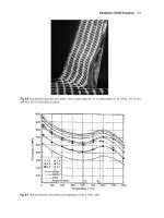
Figure 3 compares the efficiencies of the Q
n
, the median absolute deviation about
the median (MAD) and the interquartile range (IQR) measured as the percentage vari-
ance of the empirical standard deviation as a function of the sample size n, derived
from 200000 simulation runs for each n. Obviously, the Q
n
is much more efficient
than the other, ’classical’ robust scale estimators.

The higher efficiency of the Q
n
is an intuitive explanation for median compar-
isons standardized by the Q
n
having higher power than those standardized by the
MAD or the IQR if the windows are not very short. The power functions depicted in
Figure 3 for the case h = k = 15 have been derived from shifts of several heights
G = 0,1, ,6 overlaid by standard Gaussian noise, using 10000 simulation runs
each. The two-sample t-test, which is included for the reason of comparison, of-
fers under Gaussian assumptions higher power than all the median comparisons, of
course. However, Figure 3 shows that its power can drop down to zero because of
a single outlier, even if the shift is huge. To see this, a shift of fixed size 10V was
generated, and a single outlier of increasing size into the opposite direction of the
shift inserted briefly after the shift. The median comparisons are not affected by a
single outlier even if windows as short as h = k = 7 are used.
Applying the Q
n
Estimator Online 283
0 1020304050
0 20406080100
sample size
efficiency
0123456
0 20406080100
shift size
power
0 5 10 15 20
0 20406080100
outlier size

power
01234567
0 20406080100
number of deviating observations
detection rate
Fig. 3. Gaussian efficiencies (top left), power of shift detection (top right), power for a 10V-
shift in case of an outlier of increasing size (bottom left), and detection rate in case of an
increasing number of deviating observations (bottom right): Q
n
(solid), MAD (dashed), IQR
(dotted), and S
n
(dashed-dot). The two-sample t-test (thin solid) is included for the reason of
comparison.
As a final exercise, we treat shift detection in case of an increasing number of
deviating observations in the right-hand window. Since a few outliers should neither
mask a shift nor cause false detection when the signal is constant, we would like
a test to resist the deviating observations until more than half of the observations
are shifted, and to detect a shift from then on. Figure 3 shows the detection rates
calculated as the percentage of cases in which a shift was detected for h = k = 7.
Median comparisons with the Q
n
behave as desired, while a few outliers can mask
a shift when using the IQR for standardization, similar as for the t-test. This can be
explained by the IQR having a smaller breakdown point than the Q
n
and the MAD.
4 Conclusions
The proposed new update algorithm for calculation of the Q
n

scale estimator or the
Hodges-Lehmann location estimator in a moving time window shows good running
284 Robin Nunkesser, Karen Schettlinger and Roland Fried
time behavior in different data situations. The real time application of these esti-
mators, which are both robust and quite efficient, is thus rendered possible. This is
interesting for practice since the comparative studies reported here show that the
good efficiency of the Q
n
for instance improves edge detection as compared to other
robust estimators.
Acknowledgements
The financial support of the Deutsche Forschungsgemeinschaft (SFB 475, "Reduc-
tion of complexity in multivariate data structures") is gratefully acknowledged.
References
BERNHOLT, T., FRIED, R., GATHER, U. and WEGENER, I. (2006): Modified Repeated
Median Filters. Statistics and Computing, 16, 177–192.
BESPAMYATNIKH, S. N. (1998): An Optimal Algorithm for Closest-Pair Maintenance. Dis-
crete and Computational Geometry, 19 (2), 175–195.
BOVIK, A. C. and MUNSON, D. C. Jr. (1986): Edge Detection using Median Comparisons.
Computer Vision, Graphics, and Image Processing, 33, 377–389.
CROUX, C.t’and ROUSSEEUW, P. J. (1992): Time-Efficient Algorithms for Two Highly Ro-
bust Estimators of Scale. Computational Statistics, 1, 411–428.
FRIED, R. (2007): On the Robust Detection of Edges in Time Series Filtering. Computational
Statistics & Data Analysis, to appear.
GATHER, U. and FRIED, R. (2003): Robust Estimation of Scale for Local Linear Temporal
Trends. Tatra Mountains Mathematical Publications, 26, 87–101.
HWANG, H. and HADDAD, R. A. (1994): Multilevel Nonlinear Filters for Edge Detection
and Noise Suppression. IEEE Trans. Signal Processing, 42, 249–258.
JOHNSON, D. B. and MIZOGUCHI, T. (1978): Selecting the kth Element in X +Y and X
1

+
X
2
+ +X
m
. SIAM Journal on Computing, 7 (2), 147–153.
ROUSSEEUW, P.J. and CROUX, C. (1993): Alternatives to the Median Absolute Deviation.
Journal of the American Statistical Association, 88, 1273–1283.
SMID, M. (1991): Maintaining the Minimal Distance of a Point Set in Less than Linear Time.
Algorithms Review, 2, 33–44.
Classification and Retrieval of Ancient Watermarks
Gerd Brunner and Hans Burkhardt
Institute for Pattern Recognition and Image Processing, Computer Science Faculty,
University of Freiburg, Georges-Koehler-Allee 052, 79110 Freiburg, Germany
{gbrunner, Hans.Burkhardt}@informatik.uni-freiburg.de
Abstract. Watermarks in papers have been in use since 1282 in Medieval Europe. Water-
marks can be understood much in the sense of being an ancient form of a copyright signature.
The interest of the International Association of Paper Historians (IPH) lies specifically in the
categorical determination of similar ancient watermark signatures.
The highly complex structure of watermarks can be regarded as a strong and discrimina-
tive property. Therefore we introduce edge-based features that are incorporated for retrieval
and classification. The feature extraction method is capable of representing the global structure
of the watermarks, as well as local perceptual groups and their connectivity. The advantage of
the method is its invariance against changes in illumination and similarity transformations.
The classification results have been obtained with leave-one out tests and a support vec-
tor machine (SVM) with an intersection kernel. The best retrieval results have been received
with the histogram intersection similarity measure. For the 14 class problem we obtain a true
positive rate of more than 87%, that is better than any earlier attempt.
1 Introduction
Ancient watermarks served as a mark for the paper mill that made the sheet. Hence,

they served as a unique identifier and as a quality label. Nowadays, scientists from
the International Association of Paper Historians (IPH) try to identify unique wa-
termarks in order to get known the evolution of commercial and cultural exchanges
between cities in the Middle Ages (IHP 1998). The work is tedious since there are
approximately 600.000 known watermarks and their number is steadily growing.
In this paper we present a structure-based feature approach in order to automati-
cally retrieve and classify ancient watermarks. In the following we show that struc-
ture is a well suited feature to discriminate ancient watermarks.
Next, we present relevant work that is followed by a section on the actual feature
computation. In the second part of this article we show the most important results. We
summarize our contribution with a discussion of the results and a final conclusion.
238 Gerd Brunner and Hans Burkhardt
1.1 Related work
To date, there have been attempts to classify and retrieve watermark images, both by
textual- and content-based approaches. Textual approaches have been developed by
Del Marmol (1987) and Briquet (1923). As a matter of fact, pure textual classification
systems can be error prone. Watermark labels and or textual descriptions might be
very old, erroneous or just not detailed enough. Therefore, more recent attempts have
been undertaken in order to focus on the real content of watermark images. In Rauber
et al. (1997) the authors used a 16-bin large circular histogram computed around the
center of gravity of each watermark image. In addition, eight directional filters were
applied to each image and used as a feature vector. The algorithms were tested on a
small watermark database consisting of 120 images, split up into 12 different classes.
The system achieved a probability of 86% that the first retrieved image belongs to
the same class as the query image. A different approach was taken by the authors in
Riley and Eakins (2002) who used three sets of various global moment features and
three sets of component-based features. The latter set of features consists of several
shape descriptors which are extracted from various image regions.
In the following we will show that the structure of watermarks can be most effi-
ciently represented by features taken from a set of straight line segments. Therefore,

we will extract sets of segments and compute features from them on different scales.
2 Feature extraction
The geometric structure of watermarks is a strong descriptor. Therefore, we compute
a hierarchy of structural features, namely global and local ones. The former ones
depict a holistic scene representation and the latter ones take local perceptual groups
and their connectivity into account. As mentioned earlier we represent the structure
of the watermarks by straight line segments. In order to extract the line segments
we have adopted the algorithms of Pope and Lowe (1994) and Kovesi (2002). In
the first step we create an edge map with the Canny detector. Next, the algorithm
scans through the binary edge map, where the neighborhood of every edge pixel is
investigated in order to form line segments. The final segments serve as a ground
truth for the further feature computation.
Global Features
Let L = {l
i
|i = 1,2, ,N}, be a set of line segments obtained from a watermark im-
age. Then, we compute geometric properties of L such as the angles of all segments
between each other, the relative lengths of every segment and the relative Euclidean
distance between all segment mid-points.
In detail, the angle between two segments l
i
and l
j
is defined as:
cos(T
ij
)=
l
i
·l

j
||l
i
·l
j
||
2
, (1)
Classification and Retrieval of Ancient Watermarks 239
with ||·||
2
being the L2 −Norm. The angle is in the range of [−S,S]. The relative
length of a segment l
i
can be written as:
len(l
i
)=

(x
e
i
−x
b
i
)
2
+(y
e
i

−y
b
i
)
2

(x
max
−x
0
)
2
+(y
max
−y
0
)
2
, (2)
where x
b
i
, x
e
i
, y
b
i
and y
e

i
denote the coordinates of the segment’s begin and end points.
The denominator is a scaling factor in respect to the longest possible line segment
1
with (x
0
,y
0
) and (x
max
,y
max
) as the begin and end point coordinates. The Euclidean
distance between the mid-points p
c
i
and p
c
j
of the segments l
i
and l
j
is defined as
dist
c
(l
i
,l
j

)=

(x
c
j
−x
c
i
)
2
+(y
c
j
−y
c
i
)
2

(x
max
−x
0
)
2
+(y
max
−y
0
)

2
, (3)
with x
c
i
, x
c
j
, y
c
i
and y
c
j
as the coordinates of the segment mid-points. The denominator
fulfills the same scaling purpose as the one in Equation 2. Thus, the relative length
of a segment and the relative distance between two segments is limited to the range
[0,1]. The relative representation ensures invariance under isotropic scaling.
Now, that the three basic properties of a set of line segments are computed, we
can incorporate this information into Euclidean distance matrices (EDM). An EDM
is a two-dimensional array consisting of distances taken from a set of entities, that
can be coordinates or points from a feature space. Thus, an EDM incorporates dis-
tance knowledge. For our feature computation, EDMs are used in order to represent
the relative geometric connectivity for a set of straight line segments. Specifically,
we define three EDMs: one based on segment angles E
ang
(see Equation 1) a second
one based on relative segment lengths E
len
(see Equation 2) and a third one based on

relative distances between segments E
dist
(see Equation 3). The matrix of E
ang
can
be written as:
E
ang
=
⎡
⎢
⎢
⎢
⎣
e
ang
11
e
ang
12
···e
ang
1n
e
ang
21
e
ang
22
···e

ang
2n
.
.
.
.
.
.
.
.
.
.
.
.
e
ang
n1
e
ang
n2
···e
ang
nn
⎤
⎥
⎥
⎥
⎦
, (4)
and each element is computed according to

e
ang
ij
= T
i
−T
j
, (5)
where the values of T
i
and T
j
are in the range of [−S,S]. The angles are taken between
the line segments i and j. E
len
and E
dist
can be represented in a similar fashion.
Next, we compute three histograms from the previously created EDMs. The his-
tograming step is necessary since the size of the EDMs can differ, i.e. the number of
line segments is not the same for each watermark.ming step is necessary since the
size of EDMs can differ, i.e. the number of line segments is not the same for each
1
The longest possible line segment is as long as the diagonal of the image.
240 Gerd Brunner and Hans Burkhardt
watermark. The three histograms can be understood as a holistic representation of a
set of segments. The final concatenation of the three histograms resembles a global
feature and is invariant against similarity transformations.
Local features
The previously developed global features encode a complete watermark. However,

local structural information plays an important role, too. Watermarks commonly ex-
hibit certain local regularities in their structure. In order to tackle this problem we
introduce local features that are based on perceptual groups of line segments.
Therefore, we define subsets of line segments from every watermark which are
unique, eminent structural entities with well defined relations: Parallelity, Perpen-
dicularity, Diagonality (
S
4
,
3S
4
). These groups are formed according to angular re-
lations between segments and will be used in order to compute geometric relations
between their members.
The four subsets reflect line segments with certain relations. In fact, we will
extract similar features as we did in the global case. Following that methodology, we
can compute three EDMs: E
ang
∗
, E
len
∗
and E
dist
∗
, for each of the four extracted sets of
segments. Note that the ∗ is a placeholder for the four sets. Specifically, we define the
angles between two segments, the relative segment lengths and the relative distance
between two segments according to Equations 1, 2 and 3 for every subset of line
segments.

Then we create three histograms for every subset of line segments. The his-
tograms represent geometric relations of perceptual segment subsets. Since three
histograms have been formed for every set, we obtain 12 histograms in total. The
final set of local feature vectors is obtained by concatenation of all 12 histograms.
Feature representation
In our experiments we have empirically determined the best resolution for the his-
tograms. For the angle based histograms
2
we have incorporated 36 bins, that corre-
sponds to a 10
◦
resolution with respect to angles. The resolutions for every length
based histogram
3
is 15 bins, which results in a robust and compact feature. The fi-
nal feature vector is obtained by the concatenation of all global and local feature
histograms.
3 Results
3.1 Data description
The Swiss Paper Museum in Basel provided us a subset of their digital watermark
database. The database used in the subsequent experiments consists of about 1800
2
Histograms that are computed from the following EDMs: E
ang
(global features) and
E
ang
∗
(local features).
3

Histograms that are computed from the following EDMs: E
len
, E
dist
(global features) and
E
len
∗
, E
dist
∗
(local features).
Classification and Retrieval of Ancient Watermarks 241
images, split up into 14 classes. : Eagle, Anchor1, Anchor2, Coat of Arm, Circle, Bell,
Heart, Column, Hand, Sun, Bull Head, Flower, Cup and Other objects. The class
memberships are according to the Briquet catalog (Briquet 1923). Figure 1 shows
scanned sample watermark images. A detailed description of the scanning setup can
be found in Rauber (1998). In fact, the watermarks are digitized from the original
sources. Specifically, each ancient document was scanned three times (front, back
and by transparency) in order to obtain a high quality digital copy, where the last
scan contains all necessary information (Rauber 1998). A semi-automatic method,
that is describe in (Rauber 1998), delivers the final images. The method incorporates
a global contrast, contour enhancement and grey-level inversion. Figure 2 shows
sample images after the method was applied.
Fig. 1. Samples of scanned ancient watermark images (courtesy Swiss Paper Museum, Basel).
3.2 Ancient Watermark Retrieval
For retrieval we have computed the features offline for all watermarks. At retrieval
time, only the feature vector for the query watermark has to be computed. The re-
trieval results are obtained with the histogram intersection similarity measure.
Figure 3 shows a set of 10 watermark images. The first image is the query, the

second one is the identical match, indicated by the 1 above the image. The subse-
quent images are sorted in decreasing similarity, as it is indicated by the numbers
above each image. It is interesting to observe that most of the retrieved anchors show
the same orientation. A closer look at the query image reveals that it is featured with
a tiny cross atop and with cusp-like structures at the outer endings
4
. The retrieved
images clearly show that both of these small scale structures are present in all of
the displayed images. In Figure 4 we can see another retrieval result. Table 1 shows
the averaged class-wise precision and recall at N/2, where N is the number of class
4
Note, that the class Anchor1 possesses a large intra-class variation of shapes, i.e. many
anchors have no crosses or show very different endings.
242 Gerd Brunner and Hans Burkhardt
Fig. 2. Sample filigrees from the watermark database after enhancement and binarization (see
Rauber 1998). Each of the two rows shows watermarks from the same class, namely Heart
and Eagle. The samples show the large intra-class variability of the watermark database.
Fig. 3. Retrieval result obtained with our structure-based features from the class Anchor1 of
the watermark database.
Table 1.
Averaged precision and recall at N/2 for the watermark database.
Classes 1 2 3 4 5 6 7 8 9 10 11 12 13 14
N 322 115 139 71 91 44 197 126 99 33 14 31 17 416
P(N/2) .492 .243 .214 .144 .109 .244 .173 .097 .442 .068 .190 .802 .556 .283
R(N/2) .528 .139 .302 .197 .088 .182 .152 .191 .263 .061 .143 .710 .352 .361
Classification and Retrieval of Ancient Watermarks 243
Fig. 4. Retrieval result of the class Circle from the watermark database, under the usage of
global and local structural features.
members. Due to place limitations the watermark classes have been assigned a num-
ber

5
, where one refers to the class Eagle and 14 to the class Other objects.However,
we do observe some classes of worse performance. That is to a large extent due to the
high intra-class variation of the database. Figure 2 shows the large intra-class vari-
ation for two sample classes. Since CBIR performs a similarity ranking some class
members can be less similar to a certain query (from the same class) then images
from other classes. Visual inspections have shown that this argumentation holds for
the classes Eagle and Coat of Arm. The reason is that eagle motives are very com-
mon in heraldry, i.e. about half of the members of the class Coat of Arms have some
kind of eagle embedded on a shield or armorial bearings. Similar observations hold
for some other classes.
3.3 Ancient Watermark Classification
In the previous section we have retrieved watermark images. Now we want to learn
the feature distribution of every class in the feature space. Therefore, the classifi-
cation of the watermark images is treated as a learning problem. The classification
results are obtained with leave-one out tests and SVMs under the usage of different
kernel. Specifically, we have obtained the best results with the intersection kernel and
a cost parameter C = 2
20
. We have used the same features as for the retrieval task.
The feature vectors have been normalized according to zero mean and unit variance.
Table 2 shows the class-wise true and false positive rates which have been obtained
Table 2. Class-wise true positive (TP) and false positive (FP) rates for the watermark
database.
Classes 1 2 3 4 5 6 7 8 9 10 11 12 13 14 Total
TP .919 .870 .871 .465 .758 .773 .817 .865 .919 .546 .571 1.00 .824 .995 .874
FP .037 .001 .019 .012 .011 .003 .025 .008 .002 .004 .001 0 0 .008 .125
5
The class names are listed in Section 3.1.
244 Gerd Brunner and Hans Burkhardt

with a leave-one-out test. We can see that for most of the classes a high recognition
rate is achieved. In total, a 87.41% true positive rate is achieved.
4 Conclusion
The retrieval and classification of watermark images is of great importance for paper
historians. Therefore we have developed a structure-based feature extraction method
that encodes relative spatial arrangements of line segments. The method determines
relations on global and local scales. The results show that structure is a powerful de-
scriptor for the current problem. The retrieval results show that the proposed features
work very well.
Next, we have performed a classification of the watermark images. A support
vector machine with intersection kernel was able to successfully learn the character-
istics of every class. A classification rate (true positive rate) of more than 87% is an
indicator of a good performance. In future work, we would like to apply the struc-
tural features to a larger database of watermarks and investigate partial matching as
well.
References
BRIQUET, C. M. (1923): Les filigranes, Dictionnaire historique des marques de papier des
leur apparition vers 1282 jusqu’en 1600. Tome I B IV, Deuxieme edition. Verlag Von Karl
W. Hiersemann, Leipzig.
DEL MARMOL, F. (1987): Dictionnaire des filigranes classes en groupes alphabetique et
chronologiques. Namur: J. Godenne, 1900. -XIV, 192.
IHP (1998): International Standard for the Registration of Watermarks. International Associ-
ation of Paper Historians (IHP). Isbn 0250-8338.
KOVESI, P. D. (2002): Edges Are Not Just Steps. Proceedings of the Fifth Asian Conference
on Computer Vision, Melbourne, 822–827.
POPE, A. R. and LOWE, D. G. (1994): Vista: A Software Environment for Computer Vision
Research. CVPR, 768-772.
RAUBER, C. (1998): Acquisition, archivage et recherche de documents accessibles par le
contenu: Application à la gestion d’une base de données d’images de filigranes. Ph.D.
Dissertation No. 2988. University of Geneva, Switzerland.

RAUBER, C. and PUN, T. and TSCHUDIN, P. (1997): Retrieval of images from a library of
watermarks for ancient paper identification. EVA 97, Elekt. Bildverarbeitung und Kunst,
Kultur, Historie. Berlin, Germany.
RILEY, K. J. and EAKINS, J. P. (2002): Content-Based Retrieval of Historical Watermark
Images: I-tracings. Image and Video Retrieval, International Conference, CIVR. LNCS
2383, 253-261, Springer.
Collective Classification for Labeling of Places and
Objects in 2D and 3D Range Data
Rudolph Triebel
1
, Óscar Martínez Mozos
2
and Wolfram Burgard
2
1
Autonomous Systems Lab, ETH Zürich, Switzerland

2
Department of Computer Science, University of Freiburg, Germany
{omartine,burgard}@informatik.uni-freiburg.de
Abstract. In this paper, we present an algorithm to identify types of places and objects from
2D and 3D laser range data obtained in indoor environments. Our approach is a combination
of a collective classification method based on associative Markov networks together with an
instance-based feature extraction using nearest neighbor. Additionally, we show how to select
the best features needed to represent the objects and places, reducing the time needed for the
learning and inference steps while maintaining high classification rates. Experimental results
in real data demonstrate the effectiveness of our approach in indoor environments.
1 Introduction
One key application in mobile robotics is the creation of geometric maps using data
gathered with range sensors in indoor environments. These maps are usually used for

navigation and represent free and occupied spaces. However, whenever the robots
are designed to interact with humans, it seems necessary to extend these representa-
tions of the environment to improve the human-robot communication. In this work,
we present an approach to extend indoor laser-based maps with semantic terms like
“corridor”, “room”, “chair”, “table”, etc, used to annotate different places and ob-
jects in 2D or 3D maps. We introduce the instance-based associative Markov net-
work (iAMN), which is an extension of associative Markov networks together with
instance-based nearest neighbor methods. The approach follows the concept of col-
lective classification in the sense that the labeling of a data point in the space is partly
influenced by the labeling of its neighboring points. iAMNs classify the points in a
map using a set of features representing these points. In this work, we show how to
choose these features in the different cases of 2D and 3D laser scans. Experimental
results obtained in simulation and with real robots demonstrate the effectiveness of
our approach in various indoor environments.
294 Triebel et al.
2 Related work
Several authors have considered the problem of adding semantic information to 2D
maps. Koenig and Simmons (1998) apply a pre-programmed routine to detect door-
ways. Althaus and Christensen (2003) use sonar data to detect corridors and door-
ways. Moreover, Friedman et al. (2007) introduce Voronoi random fields as a tech-
nique for mapping the topological structure of indoor environments. Finally, Mar-
tinez Mozos et al. (2005) use AdaBoost to create a semantic classifier to classify free
cells in occupancy maps.
Also the problem of recognizing objects from 3D data has been studied inten-
sively. Osada et al. (2001) propose a 3D object recognition technique based on shape
distributions. Additionally, Huber et al. (2004) present an approach for parts-based
object recognition. Boykov and Huttenlocher (1999) propose an object recognition
method based on Markov random fields. Finally, Anguelov et al. (2005) present an
associative Markov network approach to classify 3D range data. This paper is based
on our previous work (Triebel et al. (2007)) which introduces the instance-based

associative Markov networks.
3 Collective classification
In most standard spatial classification methods, the label of a data point only depends
on its local features but not on the labeling of nearby data points. However, in practice
one often observes a statistical dependence of the labeling associated to neighboring
data points. Methods that use the information of the neighborhood are denoted as
collective classification techniques. In this work, we use a collective classifier based
on associative Markov networks (AMNs) (Taskar et al. (2004)), which is improved
with an instance-based nearest-neighbor (NN) approach.
3.1 Associative Markov networks
An associative Markov network is an undirected graph in which the nodes are rep-
resented by N random variables y
1
, ,y
N
. In our case, these random variables are
discrete and correspond to the semantic label of each of the data points p
1
, ,p
N
,
each represented by a vector x
i
∈R
L
of local features. Additionally, edges have asso-
ciated a vector x
ij
of features representing the relationship between the correspond-
ing nodes. Each node y

i
has an associated non-negative potential M(x
i
,y
i
). Similarly,
each edge (y
i
,y
j
) has a non-negative potential \(x
ij
,y
i
,y
j
) assigned to it. The node
potentials reflect the fact that for a given feature vector x
i
some labels are more likely
to be assigned to p
i
than others, whereas the edge potentials encode the interactions
of the labels of neighboring nodes given the edge features x
ij
. Whenever the poten-
tial of a node or edge is high for a given label y
i
or a label pair (y
i

,y
j
), the conditional
probability of these labels given the features is also high. The conditional probability
that is represented by the network is expressed as:
Collective Classification in 2D and 3D Range Data 295
P(y | x)=
1
Z
N

i=1
M(x
i
,y
i
)

(ij)∈E
\(x
ij
,y
i
,y
j
), (1)
where the partition function Z =

y



N
i=1
M(x
i
,y

i
)

(ij)∈E
\(x
ij
,y

i
,y

j
) .
The potentials can be defined using the log-linear model proposed by Taskar
et al. (2004). However, we use a modification of this model in which a weight vector
w
k
∈ R
d
n
is introduced for each class label k = 1, ,K. Additionally, a different
weight vector w
k,l

e
, with k = y
i
and l = y
j
is assigned to each edge. The potentials are
then defined as:
logM(x
i
,y
i
)=
K

k=1
(w
k
n
·x
i
)y
k
i
(2)
log\(x
ij
,y
i
,y
j

)=
K

k=1
K

l=1
(w
k,l
e
·x
ij
)y
k
i
y
l
j
, (3)
where y
k
i
is an indicator variable which is 1 if point p
i
has label k and 0, otherwise.
In a further refinement step in our model, we introduce the constraints w
k,l
e
= 0 for
k ≡ l and w

k,k
e
≥ 0. This results in \(x
ij
,k,l)=1fork ≡ l and \(x
ij
,k,k)=O
k
ij
,
where O
k
ij
≥ 1. The idea here is that edges between nodes with different labels are
penalized over edges between equally labeled nodes.
If we reformulate Equation 1 as the conditional probability P
w
(y | x), where the
parameters Z are expressed by the weight vectors w =(w
n
,w
e
), and plugging in
Equations (2) and (3), we then obtain that logP
w
(y |x) equals
N

i=1
K


k=1
(w
k
n
·x
i
)y
k
i
+

(ij)∈E
K

k=1
(w
k,k
e
·x
ij
)y
k
i
y
k
j
−logZ
w
(x). (4)

In the learning step we try to maximize P
w
(y | x) by maximizing the margin
between the optimal labeling
ˆ
y and any other labeling y (Taskar et at. (2004)). This
margin is defined by:
logP
Z
(
ˆ
y | x) −logP
Z
(y |x). (5)
The inference in the unlabeled data points is done by finding the labels y that
maximize logP
w
(y | x). We refer to Triebel et al. (2007) for more details.
3.2 Instance-based AMNs
The main drawback of the AMN classifier explained previously, which is based on
the log-linear model, is that it separates the classes linearly. This assumes that the
features are separable by hyper-planes, which is not justified in all applications. This
does not hold for instance-based classifiers such as the nearest-neighbor (NN), in
which a query data point
˜
p is assigned to the label that corresponds to the training
296 Triebel et al.
data point p whose features x are closest to the features
˜
x of

˜
p. In the learning step,
the NN classifier simply stores the entire training data set and does not compute a
reduced set of training parameters.
To combine the advantage of instance-based NN classification with the AMN
approach, we convert the feature vector
˜
x of the query point
˜
p using the transform
W : R
L
→ R
K
: W(
˜
x)=(d(
˜
x,
ˆ
x
1
), ,d(
˜
x,
ˆ
x
K
)), where K is the number of classes and
ˆ

x
k
denotes the training example with label k closest to
˜
x. The transformed features
are more easily separable by hyperplanes. Additionally, the N nearest neighbors can
be used in the transform function.
4 Feature extraction in 2D maps
In this paper, indoor environments are represented by two dimensional occupancy
grid maps (Moravec (1988)). The unoccupied cells of a grid map form an 8-connected
graph which is used as the input to the iAMN. Each cell is represented by a set of
single-valued geometrical features calculated from the 360
o
laser scan in that partic-
ular cell as shown by Martínez Mozos et al. (2005).
Three dimensional scenes are presented by point clouds which are extracted with
a laser scan. For each 3D point we computed spin images (Johnson (1997)) with a
size of 5 ×10 bins. The spherical neighborhood for computing the spin images had
a radius between 10 and 15cm, depending on the resolution of the input data.
5 Feature selection
One of the problems when classifying points represented by range data consists in
selecting the size L of the features vectors x. The number of possible features that
can be used to represent each data point is usually very large and can easily be in
the order of hundreds. This problem is known as curse of dimensionality. There are
at least two reasons to try to reduce the size of the feature vector. The most obvious
one is the computational complexity, which in our case, is also the more critical. We
have to learn an inference in networks with thousands of nodes. Another reason is
that although some features may carry a good classification when treated separately,
maybe there is a little gain if they are combined together if they have a high mutual
correlation (Theodoridis and Koutroumbas (2006)).

In our approach, the size of the feature vector for 2D data points is of the order
of hundreds. The idea is to reduce the size of the feature vectors when used with the
iAMN and at the same time try to maintain their class discriminatory information. To
do this we apply a scalar feature selection procedure which uses a class separability
criterion and incorporates correlation information. As separability criterion C,weuse
the Fisher’s discrimination ratio (FDR) extended to the multi-class case (Theodoridis
and Koutroumbas (2006)). For a scalar feature f and K classes {w
1
, ,w
K
}, C( f )
can be defined as: