Data Analysis Machine Learning and Applications Episode 2 Part 2 ppsx

Collective Classification in 2D and 3D Range Data 297
C( f )=FDR
f
=
K

i
K

j≡i
(z
i
−z
j
)
2
V
i
+ V
j
, (6)
where the subscripts i, j refer to the mean and variance of the classes w
i
and w
j
respectively. Additionally, the cross-correlation coefficient between any two features
f and g given T training examples is defined as:
U
fg
=


T
t=1
x
tf
x
tg


T
t=1
x
2
tf

T
t=1
x
2
tg
, (7)
where x
tf
denotes the value of the feature f in the training example t. Finally, the
selection of the best L features involves the following steps:
• Select the first feature f
1
as f
1
= argmax
f

C( f ).
• Select the second feature f
2
as:
f
2
= argmax
f ≡f
1

D
1
C( f )−D
2
|U
f
1
f
|

,
where D
1
and D
2
are weighting factors.
• Select f
l
, l = 1, ,L, such that:
f

l
= argmax
f ≡f
r

D
1
C( f )−
D
2
l −1
l

r=1
|U
f
r
f
|

, r = 1,2, ,l −1
6 Experiments
The approach described above has been implemented and tested in several 2D maps
and 3D scenes. The goal of the experiment is to show the effectiveness of the iAMN
in different indoor range data.
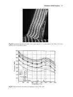
6.1 Classification of places in 2D maps
This experiment was carried out using the occupancy grid map of the building 79 at
the University of Freiburg. For efficiency reasons we used a grid resolution of 20cm,
which lead us to a graph of 8088 nodes. The map was divided into two parts, the left
one used for learning, and the right one used for classification purposes (Figure 1).

For each cell we calculate 203 geometrical features. This number was reduced to 30
applying the feature selection of Section 5. The right image of Figure 1 shows the
resulting classification with a success rate of 97.6%.
298 Triebel et al.
Fig. 1. The left image depicts the training map of building 79 at the University of Freiburg.
The right image shows the resulting classified map using an iAMN with 30 selected features.
6.2 Classification of objects in 3D scenes
In this experiment we classify 3D scans of objects that appear in a laboratory of
the building 79 of the University of Freiburg. The laboratory contain tables, chairs,
monitors and ventilators. For each object class, an iAMN is trained with 3D range
scans each containing just one object of this class (apart from tables, which may have
screens standing on top of them). Figure 2 shows three example training objects. A
complete laboratory in the building 79 of the University of Freiburg was later scanned
with a 3D laser. In this 3D scene all the objects appear together and the scene is used
as a test set. The resulting classification is shown in Figure 3. In this experiment
76.0% of the 3D points where classified correctly.
6.3 Comparison with previous approaches
In this section we compare our results with the ones obtained using other approaches
for place and object classification. First, we compare the classification of the 2D map
when using a classifier based on AdaBoost as shown by Martinez Mozos et al. (2005).
In this case we obtained a classification rate of 92.1%, in contrast with the 97.6% ob-
tained using iAMNs. We believe that the reason for this improvement is the neighbor-
ing relation between classes, which is ignored when using the AdaBoost approach. In
a second experiment, we compare the resulting classification of the 3D scene with the
one obtained when using AMN and NN. As we can see in Table 1, iAMNs perform
better than the other approaches. A posterior statistical analysis using the t-student
test indicates that the improvement is significant at the 0.05 level. We additionally
realized different experiments in which we used the 3D scans of isolated objects for
training and test purposes. The results are shown in Table 1 and they confirm that
iAMN outperform the other methods.

7 Conclusions
In this paper we propose a semantic classification algorithm that combines associa-
tive Markov networks with an instance-based approach based on nearest neighbor.
Collective Classification in 2D and 3D Range Data 299
Fig. 2. 3D scans of isolated objects used for training: a ventilator, a chair and a table with a
monitor on top.
Fig. 3. Classification of a complete 3D range scan obtained in a laboratory at the University
of Freiburg.
Table 1. Classification results in 3D data
Data set NN AMN iAMN
Complete scene 63% 62% 76%
Isolated objects 81% 72% 89%
Furthermore, we show how this method can be used to classify points described by
features extracted from 2D and 3D laser scans. Additionally, we present an approach
to reduce the number of features needed to represent each data point, while main-
taining their class discriminatory information. Experiments carried out in 2D and 3D
300 Triebel et al.
maps demonstrated the effectiveness of our approach for semantic classification of
places and objects in indoor environments.
8 Acknowledgment
This work has been supported by the EU under the project CoSy with number FP6-
004250-IP and under the project BACS with number FP6-IST-027140.
References
ALTHAUS, P. and CHRISTENSEN, H.I. (2003): Behaviour Coordination in Structured Envi-
ronments. Advanced Robotics, 17(7), 657–674.
ANGUELOV, D., TASKAR, B., CHATALBASHEV, V., KOLLER, D., GUPTA, D., HEITZ,
G. and NG, A. (2005): Discriminative Learning of Markov Random Fields for Segmen-
tation of 3D Scan Data. IEEE Computer Vision and Pattern Recognition.
BOYKOV, Y. and HUTTENLOCHER. D. P. (1999): A New Bayesian Approach to Object
Recognition. IEEE Computer Vision and Pattern Recognition.

FRIEDMAN, S., PASULA, S. and FOX, D. (2007): Voronoi Random Fields: Extracting the
Topological Structure of Indoor Environments via Place Labeling. International Joint
Conference on Artificial Intelligence.
HUBER, D., KAPURIA, A., DONAMUKKALA, R. R. and HEBERT, M. (2004): Parts-Based
3D Object Classification. IEEE Computer Vision and Pattern Recognition.
JOHNSON, A. (1997): Spin-Images: A Representation for 3-D Surface Matching. PhD thesis,
Robotics Institute, Carnegie Mellon University, Pittsburgh, PA.
KOENIG, S. and SIMMONS, R. (1998): Xavier: A Robot Navigation Architecture Based on
Partially Observable Markov Decision Process Models. In: Kortenkamp, D. and Bonasso,
R. and Murphy, R. (Eds). Artificial Intelligence Based Mobile Robotics: Case Studies of
Successful Robot Systems. MIT-Press, 91–122.
MARTINEZ MOZOS, O., STACHNISS, C. and BURGARD, W. (2005): Supervised Learning
of Places from Range Data using Adaboost. IEEE International Conference on Robotics
& Automation.
MORAVEC, H. P. (1988): Sensor Fusion in Certainty Grids for Mobile Robots. AI Magazine,
61–74.
OSADA, R., FUNKHOUSER, T., CHAZELLE, B. and DOBKIN, D. (2001): Matching 3D
Models with Shape Distributions. Shape Modeling International 154–166.
TASKAR, B., CHATALBASHEV, V. and KOLLER, D. (2004): Learning Associative Markov
Networks.International Conference on Machine Learning.
THEODORIDIS, S. and KOUTROUMBAS, K. (2006): Pattern Recognition. Academic Press,
3rd Edition, 2006.
TRIEBEL, R., SCHMIDT, R., MARTINEZ MOZOS, O. and BURGARD, W. (2007): Instace-
based AMN Classification for Improved Object Recognition in 2D and 3D Laser Range
Data. International Joint Conference on Artificial Intelligence
FSMTree: An Efficient Algorithm for Mining
Frequent Temporal Patterns
Steffen Kempe
1
, Jochen Hipp

1
and Rudolf Kruse
2
1
DaimlerChrysler AG, Group Research, 89081 Ulm, Germany
{Steffen.Kempe, Jochen.Hipp}@daimlerchrysler.com
2
Dept. of Knowledge Processing and Language Engineering,
University of Magdeburg, 39106 Magdeburg, Germany

Abstract. Research in the field of knowledge discovery from temporal data recently focused
on a new type of data: interval sequences. In contrast to event sequences interval sequences
contain labeled events with a temporal extension. Mining frequent temporal patterns from
interval sequences proved to be a valuable tool for generating knowledge in the automotive
business. In this paper we propose a new algorithm for mining frequent temporal patterns from
interval sequences: FSMTree. FSMTree uses a prefix tree data structure to efficiently organize
all finite state machines and therefore dramatically reduces execution times. We demonstrate
the algorithm’s performance on field data from the automotive business.
1 Introduction
Mining sequences from temporal data is a well known data mining task which gained
much attention in the past (e.g. Agrawal and Srikant (1995), Mannila et al. (1997),
or Pei et al. (2001)). In all these approaches, the temporal data is considered to con-
sist of events. Each event has a label and a timestamp. In the following, however,
we focus on temporal data where an event has a temporal extension. These tempo-
rally extended events are called temporal intervals. Each temporal interval can be
described by a triplet (b,e,l) where b and e denote the beginning and the end of the
interval and l its label.
At DaimlerChrysler we are interested in mining interval sequences in order to
further extend the knowledge about our products. Thus, in our domain one interval
sequence may describe the history of one vehicle. The configuration of a vehicle, e.g.

whether it is an estate car or a limousine, can be described by temporal intervals. The
build date is the beginning and the current day is the end of such a temporal interval.
Other temporal intervals may describe stopovers in a garage or the installation of
additional equipment. Hence, mining these interval sequences might help us in tasks
like quality monitoring or improving customer satisfaction.
254 Steffen Kempe, Jochen Hipp and Rudolf Kruse
2 Foundations and related work
As mentioned above we represent a temporal interval as a triplet (b,e,l).
Definition 1. (Temporal Interval) Given a set of labels l ∈ L, we say the triplet
(b,e,l) ∈ R ×R ×L is a temporal interval, if b ≤ e. The set of all temporal inter-
vals over L is denoted by I.
Definition 2. (Interval Sequence) Given a sequence of temporal intervals, we say
(b
1
,e
1
,l
1
),(b
2
,e
2
,l
2
), ,(b
n
,e
n
,l
n

) ∈ I is an interval sequence, if
∀(b
i
,e
i
,l
i
),(b
j
,e
j
,l
j
) ∈I,i = j : b
i
≤ b
j
∧e
i
≥ b
j
⇒ l
i
= l
j
(1)
∀(b
i
,e
i

,l
i
),(b
j
,e
j
,l
j
) ∈ I,i < j :
(b
i
< b
j
) ∨(b
i
= b
j
∧e
i
< e
j
) ∨(b
i
= b
j
∧e
i
= e
j
∧l

i
< l
j
)
(2)
hold. A given set of interval sequences is denoted by S.
Equation 1 above is referred to as the maximality assumption (Höppner (2002)).
The maximality assumption guarantees that each temporal interval A is maximal,
in the sense that there is no other temporal interval in the sequence sharing a time
with A and carrying the same label. Equation 2 requires that an interval sequence
has to be ordered by the beginning (primary), end (secondary) and label (tertiary,
lexicographically) of its temporal intervals.
Without temporal extension there are only two possible relations. One event is
before (or after as the inverse relation) the other or they coincide. Due to the tem-
poral extension of temporal intervals the possible relations between two intervals
become more complex. There are 7 possible relations (or 13 if one includes inverse
relations). These interval relations have been described in Allen (1983) and are de-
picted in Figure 1. Each relation of Figure 1 is a temporal pattern on its own that
consists of two temporal intervals. Patterns with more than two temporal intervals
are straightforward. One just needs to know which interval relation exists between
each pair of labels. Using the set of Allen’s interval relations I, a temporal pattern is
defined by:
Definition 3. (Temporal Pattern) A pair P =(s,R), where s :1, ,n → L and R ∈
I
n×n
,n∈ N, is called a “temporal pattern of size n” or “n-pattern”.
Fig. 1. Allen’s Interval Relations
FSMTree: An Efficient Algorithm for Mining Frequent Temporal Patterns 255
a)
b)

ABA
A eob
B
io e m
A
aime
Fig. 2. a) Example of an interval sequence: (1,4,A), (3,7,B), (7,10,A) b) Example of a temporal
pattern (e stands for equals, o for overlaps,bforbefore,mformeets,ioforis-overlapped-by,
etc.)
Figure 2.a shows an example of an interval sequence. The corresponding tempo-
ral pattern is given in Figure 2.b.
Note that a temporal pattern is not necessarily valid in the sense that it must be
possible to construct an interval sequence for which the pattern holds true. On the
other hand, if a temporal pattern holds true for an interval sequence we consider this
sequence as an instance of the pattern.
Definition 4. (Instance) An interval sequence S =(b
i
,e
i
,l
i
)
1≤i≤n
conforms to a n-
pattern P =(s, R),if∀i, j : s(i)=l
i
∧s( j)=l
j
∧R[i, j]=ir([b
i

,e
i
],[b
j
,e
j
]) with func-
tion ir returning the relation between two given intervals. We say that the interval
sequence S is an instance of temporal pattern P. We say that an interval sequence S

contains an instance of P if S ⊆ S

, i.e. S is a subsequence of S

.
Obviously a temporal pattern can only be valid if its labels have the same order as
their corresponding temporal intervals have in an instance of the pattern. Next, we
define the support of a temporal pattern.
Definition 5. (Minimal Occurrence) For a given interval sequence S a time interval
(time window) [b,e] is called a minimal occurrence of the k-pattern P (k ≥2), if (1.)
the time interval [b,e] of S contains an instance of P, and (2.) there is no proper
subinterval [b

,e

] of [b,e] which also contains an instance of P. For a given interval
sequence S a time interval [b,e] is called a minimal occurrence of the 1-pattern P,if
(1.) the temporal interval (b,e,l) is contained in S, and (2.) l is the label in P.
Definition 6. (Support) The support of a temporal pattern P for a given set of interval
sequences S is given by the number of minimal occurrences of P in S: Sup

S
(P)=
|{[b,e] : [b, e] is a minimal occurrence of P in S ∧S ∈S}|.
As an illustration consider the pattern AbeforeAin the example of Figure 2.a. The
time window [1, 11] is not a minimal occurrence as the pattern is also visible e.g. in
its subwindow [2, 9]. Also the time window [5, 8] is not a minimal occurrence. It does
not contain an instance of the pattern. The only minimal occurrence is [4,7] as the
endofthefirst and the beginning of the second A are just inside the time window.
The mining task is to find all temporal patterns in a set of interval sequences
which satisfy a defined minimum support threshold. Note that this task is closely
related to frequent itemset mining, e.g. Agrawal et al. (1993).
Previous investigations on discovering frequent patterns from sequences of tem-
poral intervals include the work of Höppner (2002), Kam and Fu (2000), Papapetrou
256 Steffen Kempe, Jochen Hipp and Rudolf Kruse
et al. (2005), and Winarko and Roddick (2005). These approaches can be divided
into two different groups. The main difference between both groups is the definition
of support. Höppner defines the temporal support of a pattern. It can be interpreted
as the probability to see an instance of the pattern within the time window if the time
window is randomly placed on the interval sequence. All other approaches count the
number of instances for each pattern. The pattern counter is incremented once for
each sequence that contains the pattern. If an interval sequence contains multiple
instances of a pattern then these additional instances will not further increment the
counter.
For our application neither of the support definitions turned out to be satisfying.
Höppner’s temporal support of a pattern is hard to interpret in our domain, as it
is generally not related to the number of instances of this pattern in the data. Also
neglecting multiple instances of a pattern within one interval sequence is inapplicable
when mining the repair history of vehicles. Therefore we extended the approach
of minimal occurrences in Mannila (1997) to the demands of temporal intervals.
In contrast to previous approaches, our support definition allows (1.) to count the

number of pattern instances, (2.) to handle multiple instances of a pattern within one
interval sequence, and (3.) to apply time constraints on a pattern instance.
3 Algorithms FSMSet and FSMTree
In Kempe and Hipp (2006) we presented FSMSet, an algorithm to find all frequent
patterns within a set of interval sequences S. The main idea is to generate all frequent
temporal patterns by applying the Apriori scheme of candidate generation and sup-
port evaluation. Therefore FSMSet consists of two steps: generation of candidate sets
and support evaluation of these candidates. These two steps are alternately repeated
until no more candidates are generated. The Apriori scheme starts with the frequent
1-patterns and then successively derives all k-candidates from the set of all frequent
(k-1)-patterns.
In this paper we will focus on the support evaluation of the candidate patterns, as
it is the most time consuming part of the algorithm. FSMSet uses finite state machines
which subsequently take the temporal intervals of an interval sequence as input to
find all instances of a candidate pattern.
It is straightforward to derive a finite state machine from a temporal pattern.
For each label in the temporal pattern a state is generated. The finite state machine
starts in an initial state. The next state is reached if we input a temporal interval that
contains the same label as the first label of the temporal pattern. From now on the
next states can only be reached if the shown temporal interval carries the same label
as the state and its interval relation to all previously accepted temporal intervals is
the same as specified in the temporal pattern. If the finite state machine reaches its
last state it also reaches its final accepting state. Consequently the temporal intervals
that have been accepted by the state machine are an instance of the temporal pattern.
The minimal time window in which this pattern instance is visible can be derived
from the temporal intervals which have been accepted by the state machine. We
FSMTree: An Efficient Algorithm for Mining Frequent Temporal Patterns 257
a)
b)
c) d)

e)
Fig. 3. a) – d) four candidate patterns of size 3 e) an interval sequence
Table 1. Set of state machines of FSMSet for the example of Figure 3. Each column shows the
new state machines that have been added by FSMSet.
1 2 3 4 5 6
S
a
() S
a
(1) S
a
(2) S
c
(3) S
c
(3,4) S
a
(5) S
a
(1,3,6)
S
b
() S
b
(1) S
b
(2) S
d
(3) S
d

(3,4) S
b
(5) S
b
(2,3,6)
S
c
() S
a
(1,3) S
c
(3,4,5)
S
d
() S
b
(2,3)
know that the time window contains an instance but we do not know whether it is
a minimal occurrence. Therefore FSMSet applies a two step approach. First it will
find all instances of a pattern using state machines. Then it prunes all time windows
which are not minimal occurrences.
To find all instances of a pattern in an interval sequence FSMSet is maintaining
asetoffinite state machines. At first, the set only contains the state machine that
is derived from the candidate pattern. Subsequently, each temporal interval from the
interval sequence is shown to every state machine in the set. If a state machine can
accept the temporal interval, a copy of the state machine is added to the set. The
temporal interval is shown only to one of these two state machines. Hence, there will
always be a copy of the initial state machine in the set trying to find a new instance
of the pattern. In this way FSMSet also can handle situations in which single state
machines do not suffice. Consider the pattern A meets B and the interval sequence

(1, 2, A), (3, 4, A), (4, 5, B). Without using look ahead a single finite state machine
would accept the first temporal interval (1, 2, A). This state machine is stuck as it
cannot reach its final state because there is no temporal interval which is-met-by
(1, 2, A). Hence the pattern instance (3, 4, A), (4, 5, B) could not be found by a single
state machine. Here this is not a problem because there is a copy of the first state
machine which will find the pattern instance.
Figure 3 and Table 1 give an example of FSMSet’s support evaluation. There are
four candidate patterns (Figure 3.a – 3.d) for which the support has to be evaluated
on the given interval sequence in Figure 3.e.
At first, a state machine is derived for each candidate pattern. The first column
in Table 1 corresponds to this initialization (state machines S
a
– S
d
). Afterwards
each temporal interval of the sequence is used as input for the state machines. The
first temporal interval has label A and can only be accepted by the state machines
S
a
() and S
b
(). Thus the new state machines S
a
(1) and S
b
(1) are added. The numbers
258 Steffen Kempe, Jochen Hipp and Rudolf Kruse
in brackets refer to the temporal intervals of the interval sequence that have been
accepted by the state machine. The second temporal interval carries again the label
A and can only be accepted by S

a
() and S
b
(). The third temporal interval has label B
and can be accepted by S
c
() and S
d
(). It also stands to the first A in the relation after
and to the second A in the relation is-overlapped-by. Hence also the state machines
S
a
(1) and S
b
(2) can accept this interval. Table 1 shows all new state machines for
each temporal interval of the interval sequence. For this example the approach of
FSMSet needs 19 state machines to find all three instances of the candidate patterns.
A closer examination of the state machines in Table 1 reveals that many state
machines show a similar behavior. E.g. both state machines S
c
and S
d
accept ex-
actly the same temporal intervals until the fourth iteration of FSMSet. Only the fifth
temporal interval cannot be accepted by S
d
. The reason is that both state machines
share the common subpattern B overlaps C as their first part (i.e. a common prefix
pattern). Only after this prefix pattern is processed their behavior can differ. Thus we
can minimize the algorithmic costs of FSMSet by combining all state machines that

share a common prefix. Combining all state machines of Figure 3 in a single data
structure leads to the prefix tree in Figure 4. Each path of the tree is a state machine.
But now different state machines can share states, if their candidate patterns share a
common pattern prefix. By using the new data structure we derive a new algorithm
for the support evaluation of candidate patterns — FSMTree.
Instead of maintaining a list of state machines FSMTree maintains a list of nodes
from the prefix tree. In the first step the list only contains the root node of the tree. Af-
terwards all temporal intervals of the interval sequence are processed subsequently.
Each time a node of the set can accept the current temporal interval its corresponding
child node is added to the set. Table 2 shows the new nodes that are added in each
step if we apply the prefix tree of Figure 4 to the example of Figure 3. Obviously the
algorithmic overhead is reduced significantly. Instead of 19 state machines FSMTree
only needs 11 nodes to find all pattern instances.
Fig. 4. FSMTree: prefix tree of state machines based on the candidates of Figure 3
FSMTree: An Efficient Algorithm for Mining Frequent Temporal Patterns 259
Table 2. Set of nodes of FSMTree for the example of Figure 3. Each column gives the new
nodes that have been added by FSMTree.
1 2 3 4 5 6
N
1
() N
2
(1) N
2
(2) N
3
(3) N
6
(3,4) N
2

(5) N
7
(1,3,6)
N
4
(1,3) N
9
(3,4,5) N
8
(2,3,6)
N
5
(2,3)
Fig. 5. Runtimes of FSMSet and FSMTree for different support thresholds.
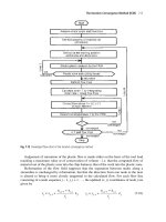
4 Performance evaluation and conclusions
In order to evaluate the performance of FSMTree in a real application scenario we
employed a dataset from our domain. This dataset contains information about the
history of 101250 vehicles. There is one sequence for each vehicle. Each sequence
comprises between 14 and 48 temporal intervals. In total, there are 345 different
labels and about 1.4 million temporal intervals in the dataset.
We performed 5 different experiments varying the minimum support threshold
from 3200 down to 200. For each experiment we measured the runtimes of FSMSet
and FSMTree. The algorithms are implemented in Java and all experiments were
carried out on a SUN Fire X2100 running at 2.2 GHz.
Figure 5 shows that FSMTree clearly outperforms FSMSet.Inthefirst experiment
FSMTree reduced the runtime from 36 to 5 minutes. The difference between FSMSet
and FSMTree even grows as the minimum support threshold gets lower. For the last
experiment FSMSet needed two days while it took FSMTree only 81 minutes. The
reason for FSMTree’s huge runtime advantage at low support threshold is that as the
support threshold decreases the number of frequent patterns increases. Consequently

the number of candidate patterns increases too. The number of candidates is the
same for FSMSet and FSMTree but FSMTree combines all patterns with common
prefix patterns. If there are more candidate patterns the chance for common prefixes
increases. Therefore FSMTree’s ability to reduce the runtime will increase (compared
to FSMSet) as the support threshold gets lower.
In this paper we presented FSMTree: a new algorithm for mining frequent tem-
poral patterns from interval sequences. FSMTree is based on the Apriori approach of
260 Steffen Kempe, Jochen Hipp and Rudolf Kruse
candidate generation and support evaluation. For each candidate pattern a finite state
machine is derived to parse the input data for instances of this pattern. FSMTree uses
aprefixtree-like data structure to efficiently organize all finite state machines. In our
application of mining the repair history of vehicles FSMTree was able to dramatically
reduce execution times.
References
AGRAWAL, R., IMIELINSKI, T. and SWAMI, A. (1993): Mining association rules between
sets of items in large databases. In: Proc. of the ACM SIGMOD Int. Conf. on Management
of Data (ACM SIGMOD ’93). 207–216.
AGRAWAL, R. and SRIKANT, R. (1995): Mining sequential patterns. In: Proc. of the 11th
Int. Conf. on Data Engineering (ICDE ’95). 3–14.
ALLEN, J. F. (1983): Maintaining knowledge about temporal intervals. Commun. ACM,
26(11):832–843.
HÖPPNER, F. and KLAWONN, F. (2002): Finding informative rules in interval sequences.
Intelligent Data Analysis, 6(3):237–255.
KAM, P S. and FU, A. W C. (2000): Discovering Temporal Patterns for Interval-Based
Events. In: Data Warehousing and Knowledge Discovery, 2nd Int. Conf., DaWaK 2000.
Springer, 317–326.
KEMPE, S. and HIPP, J. (2006): Mining Sequences of Temporal Intervals. In: 10th Europ.
Conf. on Principles and Practice of Knowledge Discovery in Databases Springer, Berlin-
Heidelberg, 569–576.
MANNILA, H., TOIVONNEN, H. and VERKAMO, I. (1997): Discovery of frequent episodes

in event sequences. Data Mining and Knowl. Discovery, 1(3):259–289.
PAPAPETROU, P., KOLLIOS, G., SCLAROFF, S. and GUNOPULOS, D. (2005): Discover-
ing frequent arrangements of temporal intervals. In: 5th IEEE Int. Conf. on Data Mining
(ICDM ’05). 354–361.
PEI, J., HAN, J., MORTAZAVI, B., PINTO, H., CHEN, Q., DAYAL, U. and HSU, M. (2001):
Prefixspan: Mining sequential patterns by prefix-projected growth. In: Proc. of the 17th
Int. Conf. on Data Engineering (ICDE ’01). 215–224.
WINARKO, E. and RODDICK, J. F. (2005): Discovering Richer Temporal Association Rules
from Interval-Based Data. In: Data Warehousing and Knowledge Discovery, 7th Int.
Conf., DaWaK 2005. Springer, Berlin-Heidelberg, 315–325.
Graph Mining: Repository vs. Canonical Form
Christian Borgelt and Mathias Fiedler
European Center for Soft Computing
c/ Gonzalo Gutiérrez Quirós s/n, 33600 Mieres, Spain


Abstract. In frequent subgraph mining one tries to find all subgraphs that occur with a user-
specified minimum frequency in a given graph database. The basic approach is to grow sub-
graphs, adding an edge and maybe a node in each step, to count the number of database graphs
containing them, and to eliminate infrequent subgraphs. The predominant method to avoid re-
dundant search (the same subgraph can be grown in several ways) is to define a canonical form
that uniquely identifies a graph up to automorphisms. The obvious alternative, a repository of
processed subgraphs, has received fairly little attention yet. However, if the repository is laid
out as a hash table with a carefully designed hash function, this approach is competitive with
canonical form pruning. In experiments we conducted, the repository-based approach could
sometimes outperform canonical form pruning by 15%.
1 Introduction
Frequent subgraph mining consists in the task to find all subgraphs that occur with a
user-specified minimum frequency in a given database of (attributed) graphs. Since
this problem appears in applications in biochemistry, web mining, and program flow

analysis, it has attracted a lot of attention, and several algorithms were proposed to
tackle it. Some of them rely on principles from inductive logic programming and
describe graphs by logical expressions (Finn et al. 1998). However, the vast ma-
jority transfers techniques developed originally for frequent item set mining. Ex-
amples include MolFea (Kramer et al. 2001), FSG (Kuramochi and Karypis 2001),
MoSS/MoFa (Borgelt and Berthold 2002), gSpan (Yan and Han 2002), Closegraph
(Yan and Han 2003), FFSM (Huan et al. 2003), and Gaston (Nijssen and Kok 2004).
A related, but slightly different approach is used in Subdue (Cook and Holder 2000).
The basic idea of these approaches is to grow subgraphs into the graphs of the
database, adding an edge and maybe a node (if it is not already in the subgraph) in
each step, to count the number of graphs containing each grown subgraph, and to
eliminate infrequent subgraphs. All found frequent subgraphs are reported (or often
only the subset of so-called closed subgraphs).
While in frequent item set mining it is trivial to ensure that each item set is
checked only once, it is a core problem in frequent subgraph mining how to avoid
230 Christian Borgelt and Mathias Fiedler
redundant search. The reason is that the same subgraph can be grown in several
ways, namely by adding the same nodes and edges in different orders. Although
multiple tests of the same subgraph do not invalidate the result of a subgraph mining
algorithm, they can be devastating for its execution time.
One of the most elegant ways to avoid redundant search is to define a canonical
description of a (sub)graph. Combined with a specific way of growing the subgraphs,
such a canonical description can be used to check whether a given subgraph has
been considered in the search before. For example, Borgelt (2006) studied a family
of such canonical forms, which comprises the special forms used in gSpan (Yan
and Han 2002) and Closegraph (Yan and Han 2003) as well as the one underlying
MoSS/MoFa (Borgelt and Berthold 2002).
However, canonical form pruning is not the only way to avoid redundant search.
A simpler and much more straightforward approach is a repository of already pro-
cessed subgraphs, against which each grown subgraph is checked. Nevertheless this

approach is rarely used, has actually not even been properly investigated yet. To
our knowledge only two existing algorithms use a repository, namely MoSS/MoFa,
which prunes with a canonical form by default, but offers the optional use of a repos-
itory, and Gaston (Nijssen and Kok 2004), in which a repository is used in the final
phase for general graphs, since Gaston’s canonical form is restricted to trees. In order
to close this gap, this paper examines repository-based pruning and compares it to
canonical form pruning. Surprisingly enough, a repository-based approach is highly
competitive and could sometimes outperform canonical form pruning by 15%.
2 Canonical form pruning
The core idea underlying a canonical form is to construct a code word that uniquely
identifies a graph up to automorphisms. The characters of this code word describe
the connection structure of the graph. If the graph is attributed (labeled), they also
comprise information about edge and node attributes. While it is straightforward
to capture the attribute information, it is less obvious how to describe the connec-
tion structure. For this, the nodes of the graph must be numbered (more generally:
endowed with unique labels), because we need to specify the source and the desti-
nation node of an edge. Unfortunately, different ways of numbering the nodes of a
graph yield different code words, because they lead to different descriptions of an
edge (simply because the indices of source and destination node differ). In addition,
the edges can be listed in different orders. Different possible solutions to these two
problems give rise to different canonical forms (see Borgelt (2006) for details).
However, given a (systematic) way of numbering the nodes of a graph and a
sorting criterion for the edges, a canonical description is derived as follows: each
numbering of the nodes yields a code word, which is the concatenation of the sorted
edge descriptions. The resulting code words are sorted lexicographically. The lexico-
graphically smallest code word is the canonical description. (It should be noted that
the graph can be reconstructed from this code word.)
Graph Mining: Repository vs. Canonical Form 231
Canonical code words are used in the search as follows: the process of growing
subgraphs is associated with a way of building code words for them. Most naturally,

the code word of a subgraph is obtained by simply concatenating the descriptions
of its edges in the order in which they are added in the search. Since each possible
subgraph needs to be checked only once, we may choose to process it only in the
node of the search tree, in which its code word (as constructed by the search) is the
canonical code word. Otherwise the subgraph (and thus the search tree rooted at it)
is pruned.
It follows that we cannot use just any possible canonical form. If extended code
words are built by appending the next edge description to the code word of the cur-
rent subgraph, then the canonical form must have the so-called prefix property:any
prefix of a canonical code word must be a canonical code word itself. Since we plan
to extend only graphs in canonical form, the prefix property is needed to ensure that
all possible subgraphs can be reached in the search. A simple way to ensure that a
canonical form has the prefix property is to confine oneself to spanning tree number-
ings of the nodes of a graph.
In a straightforward algorithm (the code words of) all possible extensions of a
subgraph are created and checked for canonical form. Extensions in canonical form
are processed further, the rest is discarded. However, canonical forms also give rise
to restrictions of the extensions of a subgraph, because for certain extensions one can
see immediately that they lead to a non-minimal code word. For the two most impor-
tant canonical forms, namely those that are based on a breadth-first (MoSS/Mofa)
and a depth-first spanning tree numbering (gSpan/Closegraph), these are (for details
see Borgelt (2006)):
• maximum source extensions
Only nodes having an index no less than the maximum source of an edge may be
extended (the source of an edge is the node with the smaller index).
• rightmost path extensions
Only the nodes on the rightmost path of the spanning tree used for numbering
the nodes may be extended (children of a node are sorted by index).
While reasons of space prevent us from reviewing details, restricted extensions are
important to mention here. The reason is that they can be exploited for the repos-

itory approach as well, because they are an inexpensive way of avoiding most of
the redundancy imminent in the search. (Note, however, that they cannot rule out all
redundancy, as there are no perfect “simple rules”.)
3 Repository of processed subgraphs
A repository of processed subgraphs is the most straightforward way of avoiding
redundant search. Every encountered frequent subgraph is stored in a data structure,
which allows us to check quickly whether a given subgraph is contained in it or not.
Whenever a new subgraph is created, this data structure is accessed and if it contains
the subgraph, we know that it has already been processed and thus can be discarded.
232 Christian Borgelt and Mathias Fiedler
Only subgraphs that are not contained in the repository are extended and, of course,
inserted into the repository.
There are two main issues one has to address when designing such a data struc-
ture. In the first place, we have to make sure that each subgraph is stored using a
minimal amount of memory, because the number of processed subgraphs is usually
huge. (This consideration may be one of the main reasons why a subgraph repository
is so rarely used.) Secondly, we have to make the containment test as fast as possible,
since it will be carried out frequently.
In order to achieve the first objective, we exploit that we only want to store graphs
that appear in at least one graph of the database (which usually resides in memory
anyway). Therefore we can store a subgraph by listing the edges of one embedding
(that is, one occurrence of the subgraph in a graph of the database). Note that it
suffices to list the edges, since the search is usually restricted to connected subgraphs
and thus the edges also identify all nodes.
1
It is pleasing to observe that this way of storing a subgraph can also make it
easier to check whether a given subgraph is equivalent to it (isomorphism test). The
rationale is to fix an order of the database graphs and to create the embeddings of all
subgraphs in this order. Then we do not store an arbitrary embedding, but one into
the first database graph it is contained in. For a new subgraph, for which we want

to know whether it is in the repository, we can then check whether the first database
graph containing it coincides with the one underlying the stored embedding. If it
does not, we already know that the subgraphs (the new one and the stored one to
which it is compared) cannot be equivalent, since equivalent subgraphs have the
same embeddings.
However, if the database graphs coincide, we carry out the actual isomorphism
test by also relying on the embeddings. We mark the embedding that is stored in the
repository (that is, its edges) in the containing database graph. Then we traverse all
embeddings of the new subgraph into the same graph
2
and check whether for any
of them all edges are marked. If such an embedding exists, the two subgraphs (the
new one and the stored one) must be equivalent, otherwise they differ. Obviously,
this isomorphism test is linear in the number of edges and thus very efficient. It
should be kept in mind, though, that it can be costly if a subgraph possesses a large
number of embeddings into the same graph, because in the worst case (that is, if
the two subgraphs are not isomorphic) all of these embeddings have to be checked.
However, our experiments showed that this is an unlikely case, since especially larger
subgraphs most of the time possess only a single embedding per database graph.
Even though an isomorphism test of the described form is fairly efficient, one
should try to avoid it. Apart from the obvious checks whether the number of nodes
and edges, the support in the graph database and the number of embeddings coin-
1
The only exception are subgraphs consisting of a single node. Fortunately, such subgraphs
need not be stored, since they cannot be created in more than one way, thus making it
unnecessary to check whether they have been processed before.
2
This is straightforward in our implementation, since in order to facilitate and accelerate
forming extensions, we keep a list of all embeddings of a subgraph.
Graph Mining: Repository vs. Canonical Form 233

cide (naturally these must all be equal for isomorphic subgraphs), we employ a hash
function that is computed from local graph properties. The basic idea is to com-
bine the node and edge attributes and the node degrees, hoping that this allows us
to distinguish non-isomorphic subgraphs. In particular, we combine for each edge
the edge attribute and the attribute and degree of the two incident nodes into a num-
ber. For each node we compute a number from the node attribute, the node degree,
the attributes of its incident edges and the attributes of the other nodes these edges
are incident to. These numbers (one for each node and one for each edge) are then
combined with the total numbers of nodes and edges to yield a hash code.
3
The computed hash code is used in the standard way to build a hash table, thus
making it possible to restrict the isomorphism test to (a subset of) the subgraphs in
one hash bin (a subset, because some collisions can be resolved by comparing the
support etc., see above). By carefully tuning the parameters of the hash function we
tried to minimize the number of collisions.
4 Comparison
Considering how canonical form pruning and repository-based pruning work, we
can make the following observations, which already give hints w.r.t. their relative
performance (and which we use to explain our experimental findings):
Canonical form pruning has the advantage that we only have to carry out one test
(for canonical form) in order to determine whether a subgraph needs to be processed
or not (even though this test can be expensive). It has the disadvantage that it is most
costly for the subgraphs that are in canonical form (and thus have to be processed),
because for these subgraphs all possibilities to construct a code word have to be tried.
For non-canonical code words the test usually terminates earlier, since it can often
construct fairly quickly a prefix that is smaller than the code word of the subgraph to
test.
Repository-based pruning has the advantage that it often allows to decide very
quickly that a subgraph has not been processed yet (for example, if a hash bin is
empty). Together with comparing the numbers of nodes and edges, the support etc.,

this suggests that a repository-based approach is fastest for subgraphs that actually
have to be processed. Only if these simple tests fail (as for equivalent subgraphs), we
have to carry out the isomorphism test.
As a consequence, we expect repository-based pruning to perform well if the
number of subgraphs to be processed is large compared to the number of subgraphs
to be discarded (as the repository is usually faster for the former).
3
A technical remark: we do not only combine these numbers by summing them and com-
puting their bitwise exclusive or, but also apply bitwise shifts of varying width in order to
cover the full range of values of (32 bit) integer numbers.
234 Christian Borgelt and Mathias Fiedler
2
2.5
3
3.5
4
4.5 5 5.5
6
20
40
60
80
time/seconds
canon. form
repository
2
2.5
3
3.5
4

4.5 5 5.5
6
20
40
60
80
time/seconds
canon. form
repository
Fig. 1. Experimental results on the IC93 data set, search time vs. minimum support in percent.
Left: maximum source extensions, right: rightmost path extensions.
5 Experiments
In order to test our repository-based pruning experimentally, we implemented it as
part of the MoSS program
4
, which is written in Java. As a test dataset (to which we
confine ourselves here due to limits of space) we used a subset of the Index Chemicus
from 1993. The results we obtained with different restricted extensions (maximum
source and rightmost path, see Section 2) are shown in Figures 1 to 3. The horizontal
axis shows the minimal support in percent.
Figure 1 shows the execution times in seconds. The upper graph refers to canon-
ical form pruning, the lower to repository-based pruning. The times do not dif-
fer much, but diverge for lower support values, reaching 15% advantage for the
repository-based approach together with maximum source extensions.
Figure 2 shows the numbers of subgraphs considered in the search and provides
a basis for explanations of the observed behavior. The graphs refer (from top to bot-
tom) to the number of generated subgraphs, the number checked for duplicates, the
number of processed subgraphs, and the number of (discarded) duplicates (difference
between the two preceding curves).
Note that about half of the work is done by minimum support pruning (which

discards all subgraphs that do not appear in the user-specified minimum number of
database graphs), as it is responsible for the difference between the two top curves.
The subgraphs discarded in this way may be unique or not—we need not care, since
they do not qualify anyway.
Canonical form or repository-based pruning only serve the purpose to get rid of
the subgraphs between the two middle curves. That the gap between them is fairly
small compared to their vertical location indicates the high quality of restricted ex-
tensions: most redundancy is already removed by them and only fairly few redundant
subgraphs still need to be detected. (Note that the gap is smaller for maximum source
extensions, which is the main reason for the usually lower execution times achieved
by this approach).
4
MoSS is available for download under the Gnu Lesser (Library) General Public License at
/>Graph Mining: Repository vs. Canonical Form 235
2
2.5
3
3.5
4
4.5 5 5.5
6
0
20
40
60
80
subgraphs/10
4
generated
dupl. tests

processed
duplicates
2
2.5
3
3.5
4
4.5 5 5.5
6
0
20
40
60
80
subgraphs/10
4
generated
dupl. tests
processed
duplicates
Fig. 2. Experimental results on the IC93 data set, numbers of subgraphs used in the search.
Left: maximum source extensions, right: rightmost path extensions.
2
2.5
3
3.5
4
4.5 5 5.5
6
0

20
40
60
80
subgraphs/10
4
generated
accesses
isom. tests
duplicates
2
2.5
3
3.5
4
4.5 5 5.5
6
0
20
40
60
80
subgraphs/10
4
generated
accesses
isom. tests
duplicates
Fig. 3. Experimental results on the IC93 data set, performance of repository-based pruning.
Left: maximum source extensions, right: rightmost path extensions.

Figure 3 finally shows the performance of repository-based pruning (mainly the
effectiveness of the hash function). All curves are the same as in the preceding fig-
ure, with the exception of the third curve from the top, which shows the number of
isomorphism tests. Subgraphs in the gap between this curve and the one above it
have to be processed and are identified as such without any isomorphism test. Only
subgraphs in the (small) gap between this curve and the bottom curve (the number of
actual duplicates) have to be identified and discarded with the help of isomorphism
tests.
Note that for a perfect hash function (which maps only equivalent subgraphs to
the same value) the two bottom curves would coincide. Note also that a canonical
form can be seen as a perfect hash function (with a range of values that does not fit
into an integer), since it uniquely identifies a graph.
6 Summary
In this paper we investigated the widely neglected possibility to avoid redundant
search in frequent subgraph mining with a repository of already encountered sub-
graphs. Even though it may be less elegant than the more popular approach of canon-
236 Christian Borgelt and Mathias Fiedler
ical forms and, of course, requires additional memory for storing the subgraphs, it
should not be dismissed too easily. If the repository is designed carefully, namely as
a hash table with a hash function computed from local graph properties, it is highly
competitive with a canonical form approach. In our experiments we observed exe-
cution times that were up to 15% lower for the repository-based approach than for
canonical form pruning, while the additional memory requirements were bearable.
References
BORGELT, C., and BERTHOLD, M.R. (2002): Mining Molecular Fragments: Finding Rel-
evant Substructures of Molecules. Proc. IEEE Int. Conf. on Data Mining (ICDM 2002,
Maebashi, Japan), 51–58. IEEE Press, Piscataway, NJ, USA
BORGELT, C., MEINL, T., and BERTHOLD, M.R. (2005): MoSS: A Program for Molec-
ular Substructure Mining. Workshop Open Source Data Mining Software (OSDM’05,
Chicago, IL), 6–15. ACM Press, New York, NY, USA

BORGELT, C. (2006): Canonical Forms for Frequent Graph Mining. Proc. 30th Ann. Conf.
of the German Classification Society (GfKl 2006, Berlin, Germany). Springer-Verlag,
Heidelberg, Germany
COOK, D.J., and HOLDER, L.B. (2000) Graph-Based Data Mining. IEEE Trans. on Intelli-
gent Systems 15(2):32–41. IEEE Press, Piscataway, NJ, USA
FINN, P.W., MUGGLETON, S., PAGE, D., and SRINIVASAN, A. (1998): Pharmacore Dis-
covery Using the Inductive Logic Programming System PROGOL. Machine Learning,
30(2-3):241–270. Kluwer, Amsterdam, Netherlands
HUAN, J., WANG, W., and PRINS, J. (2003): Efficient Mining of Frequent Subgraphs in
the Presence of Isomorphism. Proc. 3rd IEEE Int. Conf. on Data Mining (ICDM 2003,
Melbourne, FL), 549–552. IEEE Press, Piscataway, NJ, USA
INDEX CHEMICUS — Subset from 1993. Institute of Scientific Information, Inc. (ISI).
Thomson Scientific, Philadelphia, PA, USA 1993
msonscientific.com/products/indexchemicus/
KRAMER, S., DE RAEDT, L., and HELMA, C. (2001): Molecular Feature Mining in HIV
Data. Proc. 7th ACM SIGKDD Int. Conf. on Knowledge Discovery and Data Mining
(KDD 2001, San Francisco, CA), 136–143. ACM Press, New York, NY, USA
KURAMOCHI, M., and KARYPIS, G. (2001): Frequent Subgraph Discovery. Proc. 1st
IEEE Int. Conf. on Data Mining (ICDM 2001, San Jose, CA), 313–320. IEEE Press,
Piscataway, NJ, USA
NIJSSEN, S., and KOK, J.N. (2004): A Quickstart in Frequent Structure Mining Can Make
a Difference. Proc. 10th ACM SIGKDD Int. Conf. on Knowledge Discovery and Data
Mining (KDD2004, Seattle, WA), 647–652. ACM Press, New York, NY, USA
YAN, X., and HAN, J. (2002): gSpan: Graph-Based Substructure Pattern Mining. Proc. 2nd
IEEE Int. Conf. on Data Mining (ICDM 2003, Maebashi, Japan), 721–724. IEEE Press,
Piscataway, NJ, USA
YAN, X., and HAN, J. (2003): Closegraph: Mining Closed Frequent Graph Patterns. Proc.
9th ACM SIGKDD Int. Conf. on Knowledge Discovery and Data Mining (KDD 2003,
Washington, DC), 286–295. ACM Press, New York, NY, USA
Lag or Error? - Detecting the Nature of Spatial

Correlation
Mario Larch
1
and Janette Walde
2
1
ifo Institute for Economic Research at the University of Munich,
Poschingerstrasse 5, 81679 Munich, Germany

2
Department of Statistics, University of Innsbruck, Faculty of Economics and Statistics,
Universitaetsstrasse 15, 6020 Innsbruck, Austria

Abstract. Theory often suggests spatial correlations without being explicit about the exact
form. Hence, econometric tests are used for model choice. So far, mainly Lagrange Multiplier
tests based on ordinary least squares residuals are employed to decide whether and in which
form spatial correlation is present in Cliff-Ord type spatial models. In this paper, the model
selection is based both on likelihood ratio and Wald tests using estimates for the general model
and information criteria. The results of the conducted large Monte Carlo study suggest that
Wald tests on the spatial parameters after estimation of the general model are the most reliable
approach to reveal the nature of spatial correlation.
1 Introduction
Theoretical considerations frequently suggest proximity and/or similarity between
observational units as important determinant. Econometric models trying to capture
the proximity and/or similarity are referred to as ’spatial models’. Spatial models are
nowadays employed widely. Spatial correlation can have numerous reasons, e.g. in-
teraction between cross-sectional units could be due to environmental circumstances,
network externalities, market interdependencies, strategic effects such as tax set-
ting behavior and vote seeking behavior, contagion problems, population and em-
ployment growth, or the determinants of welfare expenditures. For a state-of-the-art

overview, see the book by Anselin, Florax and Rey (2004). A Google Scholar search
with the words ’spatial correlation cliff ord’ lead to 1,770 hits. This kind of spatial
models capture the proximity between observational units either by introducing a
spatially lagged (endogenous or exogenous) variable or by modeling spatial corre-
lation in the error term. In either way it is necessary to specify a weighting scheme
which specifies the proximity or similarity. A common example for the former is
the inverse distance between the capitals, whereas for the latter the membership in
regional trade groups or the common language are examples.
302 Mario Larch and Janette Walde
In most cases theory is silent about the explicit functional form of the spatial
interaction. In many applications modeling either a spatial lag in the endogenous
variable and/or a lag in the error term cooperates with the theory. Including both, a
spatially lagged endogenous variable and spatial correlation in the error term, may
therefore be useful in order to obtain white noise errors and valid hypothesis tests
for the regression parameters. The spatial autoregressive model with spatial autore-
gressive disturbances is then an obvious model to start with. However, this general
model is so far not considered as the starting point for model selection/specification.
For the choice of the econometric model, there are basically two different ap-
proaches that can be employed: the ’bottom-up’ or the ’top-down’ approach. In the
spatial econometric literature the classical specification search approach has been
predominant, which is the ’specific to general’ or ’bottom-up’ approach. First a
model without spatially lagged variables is estimated. Afterwards, Lagrange Mul-
tiplier (LM) tests for the spatial error model or the spatial lag model using ordinary
least squares (OLS) residuals are employed to decide whether spatial correlation is
present or not. If the null hypothesis of a test for a spatial autoregressive process
is rejected, a spatial variant is calculated (see Florax et al. (2003)). Florax and de
Graaff (2004) suggest to rely on the ad hoc decision rule that whichever test statistic
is greater and significantly different form zero, points to the right alternative. Note,
however, that LM tests for the spatial error and the spatial lag model exhibit power
against both alternatives.

The second approach is a ’general to specific’ or ’top-down’ approach put for-
ward by Hendry (1979), and in spatial econometrics by Florax et al. (2003). The
’top-down’ approach starts with a very general model that allows for spatial cor-
relation among various variables. A sequence of specification tests progressively
simplifies the model. We propose to use the ’top-down’ approach with the spatial
autoregressive model with spatial autoregressive disturbances as the general model.
The appropriateness of this approach is shown in a large Monte Carlo study, using
maximum likelihood (ML) and generalized method of moments (GMM) estimators.
2 Model and test statistics
We describe the estimation approaches for the spatial autoregressive model with spa-
tial autoregressive disturbances (henceforth short SARAR(1,1)), i.e. in our case the
most general model. The estimation procedure for the other models are then eas-
ily obtained by implying the restriction U = 0 for the spatial error model (abbrevi-
ated by SARAR(0,1)) and O = 0 for the spatial lag model (denoted subsequently
by SARAR(1,0)). We restrict ourself to these classes of model choice and do not
consider other possible functional forms or misspecifications (see for an analysis of
misspecification resulting form an improper weighting matrix Dubin (2003) and for
misspecification concerning the functional form McMillen (2003)).
The data generating process (DGP) for the SARAR(1,1) model considered in our
study is given by:
y=UWy+XE+u, u=OWu+H,(1)
Lag or Error? - Detecting the Nature of Spatial Correlation 303
where y is the n ×1 vector of the dependent variable, n is the sample size, X is the
n ×k matrix of the independent variables, k is the number of independent variables,
E is the k ×1 vector of coefficients, W is a given n ×n weighting matrix, U is the
coefficient of the spatially lagged dependent variable, O is the spatial error correlation
coefficient, and H is the n ×1 disturbance term. The disturbances H
i
(i = 1, , n)
are assumed to be i.i.d.(0,V

2
) with finite second and fourth moments. Further we
assume that all diagonal elements of the row normalized weighting matrix W are
zero, the absolute values of U and O are less than 1, and thus the matrices (I −UW)
and (I −UW) are nonsingular.
2.1 Estimation approaches
We use two different approaches to estimate our models: (i) Maximum Likelihood,
and (ii) GMM. For the maximum likelihood estimator two of the first order condi-
tions are employed to get the concentrated log-likelihood function LL
c
=
Fkt(U,O;X,y). This is a non-linear function in the two parameters U and O (Anselin
(1988a)). The standard errors of all the estimators are obtained via the information
matrix.
The second approach is based on generalized method of moments (GMM). The
GMM estimator is a two-stage least squares procedure that uses additional moment
conditions to estimate the spatial parameters. To account for the endogeneity of Wy,
all independent variables as well as the once and twice spatially lagged independent
variables ([X, WX, W
2
X]) serve as instruments as recommended by Kelejian and
Prucha (1999). Kelejian and Prucha (1999) proposed a three-step procedure. In the
first step a consistent estimate for the residuals is obtained by two-stage least squares
(2SLS). These residuals are used in the moment conditions to estimate the spatial cor-
relation coefficient of the error term. In the final step, a Cochrane-Orcutt type trans-
formation is applied and the parameters are estimated by 2SLS on the transformed
values. Lee (2003) proved that these instruments do not lead to asymptotically effi-
cient parameter estimates. He suggests to use H =(I −OW)[X,W(I −UW)
−1
X

ˆ
E] as
instruments, where
ˆ
E are the estimates from the first-step regression. We apply these
optimal instruments by replacing U and O with their estimates from the first step.
The standard errors for the regression coefficients and the coefficient of the spatially
lagged dependent variable are readily obtained from the last stage regression. How-
ever, in order to obtain the standard error for the spatial error parameter, we have to
apply the estimator suggested in Kelejian and Prucha (2006).
2.2 Applied tests for model selection
First the ’specific to general’ approaches are described. These tests start from the
most simple model and turn to more complicated ones if the test statistic rejects the
simple model. In the applied framework the most simple model is one without spatial
lag and spatial error, i.e. OLS regression.
Available tests are mainly LM tests, which only rely on the estimates of the
model unter the null hypothesis. Basically the LM tests suggested by Anselin et
304 Mario Larch and Janette Walde
al. (1996) are implemented. As the LM tests are based on OLS resiudals,
ˆ
u denotes
the estimated residuals from the OLS regression, and
ˆ
V
2
=(1/n)
ˆ
u

ˆ

u.Further,we
have to distinguish whether we assume the second spatial parameter to be zero or
not. The following definitions will simplify the expressions: T = tr((W

+ W)W),
M = I −X(X

X)
−1
X

,
ˆ
J
UE
=
1
n
ˆ
V
2
[(WX
ˆ
E)

M(WX
ˆ
E)+T
ˆ
V

2
]. Now the following tests
can be conducted:
Model: y = XE +u, assumption: U = 0,H
0
: O = 0(2)
LM
O
=
( ˆu

W ˆu/
ˆ
V
2
)
2
T
.
Model: y = XE +u, assumption: O = 0,H
0
: U = 0(3)
LM
U
=
( ˆu

Wy/
ˆ
V

2
)
2
n
ˆ
J
UE
.
Model: y = UWy+XE +u,H
0
: O = 0(4)
LM
∗
O
=
[ ˆu

W ˆu/
ˆ
V
2
−T(n
ˆ
J
UE
)
−1
ˆu

Wy/

ˆ
V
2
]
2
T[1 −T (n
ˆ
J
UE
)]
−1
.
Model: y = XE +u,u = OWu + H,H
0
: U = 0(5)
LM
∗
U
=
[ ˆu

Wy/
ˆ
V
2
− ˆu

W ˆu/
ˆ
V

2
]
2
n
ˆ
J
UE
−T
.
LM tests for U and O in the case of spatial correlation in the error term or in the
dependent variable respectively, which are assumed to be estimated, were derived by
Anselin (1988b):
LM
A
O
=
[ˆu

W
2
ˆu/
ˆ
V
2
]
2
T
22
−(T
21A

)
2
ˆvar(
ˆ
U)
, (6)
LM
A
U
=
[ˆu

B

BW
1
y]
2
H
rho
−H
TU
ˆvar(
ˆ
T)H

TU
, (7)
where T
21A

= tr[W
2
W
1
A
−1
+W

2
W
1
A
−1
], A = I −
ˆ
UW
1
, T

=(E

OV12)

, B = I −
ˆ
OW
2
,
H
U

= trW
2
+ tr(BW B
−1
)

(BW B
−1
)+
1
V
2
(BW X E)

(BW X E) and H

TU
=
⎛
⎝
1
V
2
(BX)

BW X E
tr(WB
−1
)


BW B
−1
+trWW B
−1
0
⎞
⎠
, with ˜var(
˜
T) as the estimated variance matrix
for the parameter vector T in the null model.
Besides the described LM test we calculate likelihood ratio (LR) tests. There-
fore one needs to calculate both the restricted and the unrestricted model, i.e. LR =
−2(LL
r
−LL
ur
), where LL
ur
(LL
r
) denotes the value of the maximized log-likelihood
of the unrestricted (restricted) model.
Third, we calculate Wald tests for both the MLE and the GMM approach. The
SARAR(1,1) model has to be estimated in order to test against more sparse variants.
Hence, these tests are in the vein of a ’general to specific’ methodology. Given the
Lag or Error? - Detecting the Nature of Spatial Correlation 305
estimates for the general model, we can conduct the Wald test for U and O: W
U
=

ˆ
U/
ˆ
V
U
and W
O
=
ˆ
O/
ˆ
V
O
, where
ˆ
U and
ˆ
O are the estimates of the general model under
consideration, and
ˆ
V
U
and
ˆ
V
O
are the estimated standard errors thereof. Note that with
the estimates of the SARAR(1,1) model we can conduct a test for joint significance
of U and O for both, the MLE and the GMM estimators.
Fourth, widely used information criteria are implemented in order to obtain the

true DGP. The Akaike information criterion (AIC), the bias corrected Akaike crite-
rion (AIC
c
), and the Schwartz information criterion (BIC) are calculated (e.g., Belitz
and Lang (2006)).
3 Monte Carlo study
All test evaluations are done using a sample size of 400. The regression coefficient
vector E is set to be (1,1). The independent variable is drawn randomly from the
uniform distribution between zero and twenty. The remainder noise is normally dis-
tributed with mean zero and variance one. For each setting of the true DGP 1000
Monte Carlo data sets are calculated which leads to a 95% confidence interval for
the nominal significance level of 5%±1.35%.
Two different weighting schemes are employed. The units are ordered regularly
in a square grid of size
√
n×
√
n. The first weighting matrix uses the Moore (Queen,
e.g., Anselin (1988b)) neighborhood with radius r = 1. After row normalizing the
matrix, the weighting matrix W is obtained, and denoted henceforth as W
1
. As sec-
ond weighting matrix (W
2
) the distance d
ij
between observation units i and j is com-
puted and the elements of the weighting matrix are calculated as 1/d
ij
if i ≡ j.The

diagonal elements are set to zero. In order to limit the neighboring influence, addi-
tionally the elements of the weighting matrix are set to zero if the distance is greater
than 7.1 (which corresponds to a radius of 5). Hence, the weighting matrix based on
the Moore neighborhood (W
1
) is sparser and demonstrates less spatial connectivity
than the one based on the distance (W
2
).
In order to obtain the power function the true spatial correlation parameters
are varied in the following way (U,O)=(0,0.5),(0.05, 0.5), (0.1, 0.5), (0.15, 0.5),
(0.2,0.5),(0.5,0),(0.5,0.05),(0.5,0.1),(0.5,0.15), (0.5, 0.2
).
4 Results
Let us first analyze the experiments with SARAR(1,1) as true DGP. In order to obtain
the size and the power of the Wald test the spatial parameter O (U)isfixed at the value
of 0.5. The second spatial parameter U (O) is varied from 0 to 0.2. The actual size
of the Wald test with the null hypothesis H
0
: U = 0(H
0
: O = 0) is not significantly
different from the nominal size of 5%. The joint hypothesis test supports the alter-
native hypothesis with 100% as well as the Wald test for the corresponding second
spatial parameter O(U). Hence, the correct more parsimonious model under the null
hypothesis is detected accordingly.