Data Analysis Machine Learning and Applications Episode 2 Part 3 pps

306 Mario Larch and Janette Walde
When the null hypothesis is tested whether the spatial correlation parameter U
is zero in the presence of spatial correlation in the error term the Wald test has a
very good power although the power is higher with the sparser weighting matrix.
The latter characteristic is a general feature for all conducted tests. The power for
the spatial error parameter in the presence of a non-zero spatial lag parameter is
lower. However, the power of the Wald test in this circumstances is (much) greater
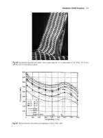
than the power achievable by using Lagrange Multiplier tests. In Figure 1c the best
performing LM test is plotted, i.e. LM
A
. All LM tests relying on OLS residuals fail
seriously to detect the true DGP.
Comparable to the performance of the Wald test based on MLE estimates is the
Wald test based on GMM estimates but only in detecting the significant lag parameter
in the presence of a significant spatial error parameter. In the reverse case the Wald
test using GMM estimates is much worse.
As a further model selection approach the performance of information criteria
is analyzed. The performance of the classical Akaike information criterion and the
bias corrected AIC are almost identical. In Figure 1d the share of cases in which
AIC/AIC
c
identifies the correct DGP is plotted on the y-axis. All information cri-
teria fail in more than 15% of the cases to identify the correct more parsimonious
model, i.e. SARAR(1,0) or SARAR(0,1) instead of SARAR(1,1). However, in the
remaining experiments (U = 0.05, ,0.2orO = .05, ,0.2) AIC/AIC
c
is compara-
ble to the performance of the Wald test. BIC performs better than AIC/AIC
c
to detect
SARAR(1,0) or SARAR(0,1) instead of SARAR(1,1) but much worse in the remain-

ing experiments.
In order to be able to propose a general procedure for model selection the ap-
proach must also be suitable if the true DGP is SARAR(1,0) or SARAR(0,1). In this
case the Wald test based on the general model has again the appropriate size and a
very good power. Further the sensitivity on different weighting matrices is less se-
vere. However, the power is smallest for the test with the null hypothesis H
0
: O = 0
and with distance as weighting scheme W
2
. The Wald test using GMM estimates is
again comparable when testing for the spatial lag parameter but worse when testing
for the spatial error parameter.
Not significantly different from the power function of the Wald test based on the
general model are both LM statistics based on OLS residuals. However, in this case
LM
A
fails to identify the correct DGP.
The Wald test outperforms the information criteria regarding the identification of
SARAR(1,0) or SARAR(0,1). If OLS is the DGP, the correct model is chosen only
about two thirds of the time by AIC/AIC
c
but comparably often to Wald by BIC. If
SARAR(1,0) is the data generating process all information criteria perform poorer
than the Wald test independent of the underlying weighting scheme. If the
SARAR(0,1) is the data generating process, BIC is worse than the Wald test, and
AIC/AIC
c
has a slightly higher performance for small values of the spatial parame-
ter but is outperformed by the Wald test for higher values of the spatial parameters.

For the sake of completeness it is noted that no valid model selection can be con-
ducted using likelihood ratio tests.
Lag or Error? - Detecting the Nature of Spatial Correlation 307
0 0.05 0.1 0.15 0.2
0
0.1
0.2
0.3
0.4
0.5
0.6
0.7
0.8
0.9
1
U,O
power
a) SARAR(1,1): MLE Wald
W
1
W
1
, O=0.5
W
1
W
1
, U=0.5
W
2

W
2
, O=0.5
W
2
W
2
, U=0.5
0 0.05 0.1 0.15 0.2
0
0.1
0.2
0.3
0.4
0.5
0.6
0.7
0.8
0.9
1
U,O
power
b) SARAR(1,1): GMM opt.inst. Wald
W
1
W
1
, O=0.5
W
1

W
1
, U=0.5
W
2
W
2
, O=0.5
W
2
W
2
, U=0.5
0 0.05 0.1 0.15 0.2
0
0.1
0.2
0.3
0.4
0.5
0.6
0.7
0.8
0.9
1
U,O
power
c) SARAR(1,1): LM
A
W

1
W
1
, O=0.5
W
1
W
1
, U=0.5
W
2
W
2
, O=0.5
W
2
W
2
, U=0.5
0 0.05 0.1 0.15 0.2
0
0.1
0.2
0.3
0.4
0.5
0.6
0.7
0.8
0.9

1
U,O
correct model choice [%]
d) SARAR(1,1): AIC
W
1
W
1
, O=0.5
W
1
W
1
, U=0.5
W
2
W
2
, O=0.5
W
2
W
2
, U=0.5
Fig. 1. a) Power of the Wald test based on the general model and MLE estimates. b) Power
of the Wald test based on the general model and GMM estimates. c) Power of the Lagrange
Multiplier test using LM
A
as test statistic. d) Correct model choice of the better performing
information criterion (AIC/AIC

c
).
To conclude, we find that the ’general to specific’ approach is the most suitable
procedure to identify the correct data generating process (DGP) regarding Cliff-Ord
type spatial models. Independent whether the true DGP is a SARAR(1,1),
SARAR(1,0), SARAR(0,1), or just a regression model without any spatial corre-
lation, the general model should be estimated and the Wald tests conducted. The
chance to identify the true DGP is than higher compared to the alternative model
choice criteria based on the LM tests, LR tests or on information criteria like AIC,
AIC
c
or BIC.
References
ANSELIN, L. (1988a): Lagrange Multiplier Test Diagnostics for Spatial Dependence and Spa-
tial Heterogeneity. Geographical Analysis, 20, 1–17.
ANSELIN, L. (1988b): Spatial Econometrics: Methods and Models. Kluwer Academic Pub-
lishers, Boston.
ANSELIN, L., BERA, A., FLORAX, R. and YOON, M. (1996): Simple Diagnostic Tests for
Spatial Dependence, Regional Science and Urban Economics, 26, 77–104.
308 Mario Larch and Janette Walde
ANSELIN, L., FLORAX, R. and REY, S. (2004): Advances in Spatial Econometrics. Springer,
Berlin.
BELITZ, C. and LANG, S. (2006), Simultaneous selection of variables and smoothing param-
eters in geoadditive regression models. In H J. Lenz, and R. Decker (Eds.):Advances in
Data Analysis. Springer, Berlin-Heidelberg, forthcoming.
DUBIN, R. (2003): Robustness of Spatial Autocorrelation Specifications: Some Monte Carlo
Evidence, Journal of Regional Science, 43, 221–248.
FLORAX, R.J., and DE GRAAFF, T. (2004): The Performance of Diagnostic Tests for Spatial
Dependence in Linear Regression Models: A Meta-Analysis of Simulation Studies. In:
L. Anselin, R.J. Florax, and S.J. Rey (Eds.): Advances in Spatial Econometrics - Method-

ology, Tools and Applications. Springer, Berlin-Heidelberg, 29-65.
FLORAX, R.J., and REY, S.J. (1995): The Impacts of Misspecified Spatial Interaction in Lin-
ear Regression Models. In: L. Anselin, R.J. Florax, and S.J. Rey (Eds.): New Directions
in Spatial Econometrics. Springer, Berlin-Heidelberg, 111-135.
FLORAX, R.J., FOLMER, H., and REY, S.J. (2003): Specification Searches in Spatial Econo-
metrics: The Relevance of HendryŠs Methodology, Regional Science and Urban Eco-
nomics, 33, 557–579.
HENDRY, D. (1979): Predictive Failure and Econometric Modelling in Macroeconomics: The
Transactions Demand for Money. In: P. Ormerod (Ed.): Economic Modelling. Heine-
mann, London, 217-242.
KELEJIAN, H., and PRUCHA, I. (1999): A Generalized Moments Estimator for the Autore-
gressive Parameter in a Spatial Model, International Economic Review, 40, 509–533.
KELEJIAN, H., and PRUCHA, I. (2006): Specification and Estimation of Spatial Autore-
gressive Models with Autoregressive and Heteroskedastic Disturbances, unpublished
manuscript, University of Maryland.
LEE, L. (2003): Best Spatial Two-Stage Least Squares Estimators for a Spatial Autoregressive
Model with Autoregressive Disturbances, Econometric Reviews, 22, 307–335.
MCMILLEN, D. (2003): Spatial Autocorrelation or Model Misspecification?, International
Regional Science Review, 26, 208–217.
Segmentation and Classification
of Hyper-Spectral Skin Data
Hannes Kazianka
1
, Raimund Leitner
2
and Jürgen Pilz
1
1
University of Klagenfurt, Institute of Statistics, Alpen-Adria-Universität Klagenfurt,
Universitätsstraße 65-67, 9020 Klagenfurt, Austria

{hannes.kazianka, juergen.pilz} @uni-klu.ac.at
2
CTR Carinthian Tech Research AG, Europastraıe 4/1, 9524 Villach, Austria

Abstract. Supervised classification methods require reliable and consistent training sets. In
image analysis, where class labels are often assigned to the entire image, the manual genera-
tion of pixel-accurate class labels is tedious and time consuming. We present an independent
component analysis (ICA)-based method to generate these pixel-accurate class labels with
minimal user interaction. The algorithm is applied to the detection of skin cancer in hyper-
spectral images. Using this approach it is possible to remove artifacts caused by sub-optimal
image acquisition. We report on the classification results obtained for the hyper-spectral skin
cancer data set with 300 images using support vector machines (SVM) and model-based dis-
criminant analysis (MclustDA, MDA).
1 Introduction
Hyper-spectral images consist of several, up to hundred, images acquired at different
- mostly narrow band and contiguous - wavelengths. Thus, a hyper-spectral image
contains pixels represented as multidimensional vectors with elements indicating the
reflectivity at a specific wavelength. For a contiguous set of narrow band wavelengths
these vectors correspond to spectra in the physical meaning and are equal to spectra
measured with e.g. spectrometers.
Supervised classification of hyper-spectral images requires a reliable and consistent
training set. In many applications labels are assigned to the full image instead of to
each individual pixel even if instances of all the classes occur in the image. To obtain
a reliable training set it may be necessary to label the images on a pixel by pixel basis.
Manually generating pixel-accurate class labels requires a lot of effort; cluster-based
automatic segmentation is often sensitive to measurement errors and illumination
problems. In the following we present a labelling strategy for hyper-spectral skin
cancer data that uses PCA, ICA and K-Means clustering. For the classification of
unknown images, we compare support vector machines and model-based discrimi-
nant analysis.

246 Hannes Kazianka, Raimund Leitner and Jürgen Pilz
Section 2 describes the methods that are used for the labelling approach. The classi-
fication algorithms are discussed in Section 3. In Section 4 we present the segmen-
tation and classification results obtained for the skin cancer data set and Section 5 is
devoted to discussions and conclusions.
2 Labelling
Hyper-spectral data are highly correlated and contain noise which adversely affects
classification and clustering algorithms. As the dimensionality of the data equals the
number of spectral bands, using the full spectral information leads to computational
complexity. To overcome the curse of dimensionality we use PCA to reduce the di-
mensions of the data, and inherently also unwanted noise. Since different features of
the image may have equal score values for the same principal component, an addi-
tional feature extraction step is proposed. ICA makes it possible to detect acquisition
artifacts like saturated pixels and inhomogeneous illumination. Those effects can be
significantly reduced in the spectral information giving rise to an improved segmen-
tation.
2.1 Principal Component Analysis (PCA)
PCA is a standard method for dimension reduction and can be performed by sin-
gular value decomposition. The algorithm gives uncorrelated principal components.
We assume that those principal components that correspond to very low eigenvalues
contribute only to noise. As a rule of thumb, we chose to retain at least 95% of the
variability which led to selecting 6-12 components.
2.2 Independent Component Analysis (ICA)
ICA is a powerful statistical tool to determine hidden factors of multivariate data. The
ICA model assumes that the observed data, x, can be expressed as a linear mixture
of statistically independent components, s. The model can be written as
x = As
where the unknown matrix A is called the mixing matrix. Defining W as the unmixing
matrix we can calculate s as
s = Wx.

As we have already done a dimension reduction, we can assume that noise is neg-
ligible and A is square which implies W = A
−1
. This significantly simplifies the
estimation of A and s. Providing that no more than one independent component has
Gaussian distribution, the model can be uniquely estimated up to scalar multipliers.
There exists a variety of different algorithms for fitting the ICA model. In our work
we focused on the two most popular implementations which are based on maximisa-
tion of non-Gaussianity and minimisation of mutual information respectively: Fas-
tICA and FlexICA.
Segmentation and Classification of Hyper-Spectral Skin Data 247
FastICA
The FastICA algorithm developed by Hyvärinen et al. (2002) uses negentropy, J (y),
as a measure of Gaussianity. Since negentropy is zero for Gaussian variables and
always nonnegative one has to maximise negentropy in order to maximise non-
Gaussianity. To avoid computation problems the algorithm uses an approximation
of negentropy: If G denotes a nonquadratic function and we want to estimate one
independent component s we can approximate
J(y) ≈[E
{
G(y)
}
−E
{
G(Q)
}
]
2
,
where Q is a standardised Gaussian variable and y is an estimate of s. We adopt to use

G(y)=logcoshy since this has been shown to be a good choice. Maximisation di-
rectly leads to a fixed-point iteration algorithm that is 20−50 times faster than other
ICA implementations. To estimate several independent components a deflationary
orthogonalisation method is used.
FlexICA
Mutual information is a natural measure of information that members of a set of
random variables have on the others. Choi et al. (2000) proposed an ICA algorithm
that attempts to minimise this quantity. All independent components are estimated
simultaneously using a natural gradient learning rule with the assumption that the
source signals have the generalized Gaussian distribution with density
q
i
(y
i
)=
r
i
2V
i
*(1/r
i
)
exp

−
1
r
i





y
i
V
i




r
i

.
Here r
i
denotes the Gaussian exponent which is chosen in a flexible way depending
on the kurtosis of the y
i
.
2.3 Two-Stage K-Means clustering
From a statistical point of view it may be inappropriate to use K-means clustering
since K-means cannot use all the higher order information that ICA provides. There
are several approaches that avoid using K-means, for example Shah et al. (2005) pro-
posed the ICA mixture model (ICAMM). However, for large images this algorithm
fails to converge. We developed a 2-stage K-means clustering strategy that works
particularly well with skin data. The choice of 5 resp. 3 clusters for the K-means
algorithm has been determined empirically for the skin cancer data set.
1. Drop ICs that contain a high amount of noise or correspond to artifacts.
2. Perform K-means clustering with 5 clusters.

3. Those clusters that correspond to healthy skin are taken together into one cluster.
This cluster is labelled as skin.
4. Perform a second run of K-means clustering on the remaining clusters (inflamed
skin, lesion, etc.). This time use 3 clusters. Label the clusters that correspond to
the mole and melanoma centre as mole and melanoma. The remaining clusters
are considered to be ‘regions of uncertainty’.
248 Hannes Kazianka, Raimund Leitner and Jürgen Pilz
3 Classification
This section describes the classification methods that have been investigated. The
preprocessing steps for the training data are the same as in the segmentation task:
Dimension reduction using PCA and feature extraction performed by ICA. Using
the Bayesian Information Criterion (BIC), the data were reduced to 6 dimensions.
3.1 Mixture Discriminant Analysis (MDA)
MDA assumes that each class j can be modelled as a mixture of R
j
subclasses.
The subclasses have a multivariate Gaussian distribution with mean vector z
jr
, r =
1, ,R
j
, and covariance matrix 6, which is the same for all classes. Hence, the
mixture model for class j has the density
m
j
(x)=
|
2S6
|
−

1
2
R
j

r=1
S
jr
exp

−

x −z
jr

6
−1

x −z
jr

2

,
where S
jr
denote the mixing probabilities for the j-th subclass,

R
j

r=1
S
jr
= 1. The
parameters T =

z
jr
,6,S
jr

can be estimated using an EM-algorithm or, as Hastie et
al. (2001) suggest, using optimal scoring. It is also possible to use flexible discrim-
inant analysis (FDA) or penalized discriminant analysis (PDA) in combination with
MDA. The major drawback of this classification approach is that, similar to LDA
which is also described in Hastie et al. (2001), the covariance matrix is fixed for all
classes and the number of subclasses for each class has to be set in advance.
3.2 Model-based Discriminant Analysis (MclustDA)
MclustDA, proposed by Fraley et al. (2002), extends MDA in a way that the covari-
ance in each class is parameterized using the eigenvalue decomposition
6
r
= O
r
D
r
A
r
D
T

r
, r = 1, ,R
j
.
The volume of the component is controlled by O
r
, A
r
defines the shape and D
r
is
responsible for the orientation. The model selection is done using the BIC and the
maximum likelihood estimation is performed by an EM-algorithm.
3.3 Support Vector Machines (SVM)
The aim of support vector machines is to find a hyperplane that optimally separates
two classes in a high-dimensional feature space induced by a Mercer kernel K (x,z).
In the L
2
-norm case the Lagrangian dual problem is to find O
∗
that solves the follow-
ing convex optimization problem:
max
O
m

i=1
O
i
−

1
2
m

i=1
m

j=1
O
i
O
j
y
i
y
j

K (x
i
,x
j
)+
1
C
G
ij

s.t.
m


i=1
O
i
y
i
= 0, O
i
≥ 0,
Segmentation and Classification of Hyper-Spectral Skin Data 249
where x
i
are training points belonging to classes y
i
. The cost parameter C and the
kernel function have to be chosen to suit to the problem. It is also possible to use
different cost parameters for unbalanced data as was suggested by Veropoulos et al.
(1999).
Although SVMs were originally designed as binary classifiers, there exists a vari-
ety of methods to extend them to k > 2 classes. In our work we focused on one-
against-all and one-against-one SVMs. The one-against-all formulation trains each
class against all remaining classes resulting in k binary SVMs. The one-against-one
formulation uses
k(k−1)
2
SVMs, each separating one class from one another.
4 Results
A set of 310 hyper-spectral images (512 ×512 pixels and 300 spectral bands) of
malign and benign lesions were taken in clinical studies at the Medical University
Graz, Austria. They are classified as melanoma or mole by human experts on the
basis of a histological examination. However, in our survey we distinguish between

three classes, melanoma, mole and skin, since all these classes typically occur in the
images. The segmentation task is especially difficult in this application: We have
to take into account that melanoma typically occurs in combination with mole.To
reduce the number of outliers in the training set we define a ‘region of uncertainty’
as a transition region between the kernels of mole and melanoma and between the
lesion and the skin.
4.1 Training
Figures 1(b) and 1(c) display the first step of the K-Means strategy described in Sec-
tion 2.3. The original image displayed in Figure 1(a) shows a mole that is located
in the middle of a hand. For PCA-transformed data, as in Figure 1(b), the algorithm
performs poorly and the classes do not correspond to lesion, mole and skin regions
(left and bottom). Even the lesion is in the same class together with an illumination
problem. If the data is also transformed using ICA, as in Figure 1(c), the lesion is
already identified and there exists a second class in the form of a ring around the
lesion which is the desired ‘region of uncertainty’. The other classes correspond to
wrinkles on the hand.
Figure 1(d) shows the second K-Means step for the PCA transformed data. Although
the second K-Means step makes it possible to separate the lesion from the illumina-
tion problem it can be seen that the class that should correspond to the kernel of the
mole is too large. Instances from other classes are present in the kernel. The second
K-Means step with the ICA preprocessed data is shown in Figure 1(e). Not only the
kernel is reliably detected but there also exists a transition region consisting of two
classes. One class contains the border of the lesion. The second class separates the
kernel from the remaining part of the mole.
We believe that the FastICA algorithm is the most appropriate ICA implementation
250 Hannes Kazianka, Raimund Leitner and Jürgen Pilz
(a) (b) (c)
(d) (e)
Fig. 1. The two iteration steps of the K-Means approach for both PCA ((b) and (d)) and
ICA ((c) and (e)) are displayed together with the original image (a). The different gray levels

indicate the cluster the pixel has been assigned to.
for this segmentation task. The segmentation quality for both methods is very simi-
lar, however the FastICA algorithm is faster and more stable.
To generate a training set of 12.000 pixel spectra per class we labelled 60 mole im-
ages and 17 melanoma images using our labelling approach. The pixels in the train-
ing set are chosen randomly from the segmented images.
4.2 Classification
In Table 1 we present the classification results obtained for the different classifiers
described in Section 3. As a test set we use 57 melanoma and 253 mole images. We
use the output of the LDA classifier as a benchmark.
LDA turns out to be the worst classifier for the recognition of moles. Nearly one half
of the mole images are misclassified as melanoma. On the other hand LDA yields
excellent results for the classification of melanoma, giving rise to the presumption
that there is a large bias towards the melanoma class. With MDA we use three sub-
classes in each class. Although both MDA and LDA keep the covariance fixed, MDA
models the data as mixture of Gaussians leading to a significantly higher recognition
rate compared to LDA. Using FDA or PDA in combination with MDA does not im-
prove the results. MclustDA performs best among these classifiers. Notice however,
that BIC overestimates the number of subclasses in each class which is between 14
and 21. For all classes the model with varying shape, varying volume and varying
Segmentation and Classification of Hyper-Spectral Skin Data 251
Table 1. Recognition rates obtained for the different classifiers
Pre-Proc. Class
MDA MclustDA LDA
FlexICA
Mole
84.5% 86.5% 56.1%
Melanoma
89.4% 89.4% 98.2%
FastICA

Mole
84.5% 87.7% 56.1%
Melanoma
89.4% 89.4% 98.2%
Pre-Proc. Class
OAA-SVM OAO-SVM unbalanced SVM
FlexICA
Mole
72.7% 69.9% 87.7%
Melanoma
92.9% 94.7% 89.4%
FastICA
Mole
71.5% 69.9% 87.3%
Melanoma
92.9% 94.7% 89.4%
orientation of the mixture components is chosen. This extra flexibility makes it pos-
sible to outperform MDA even though only half of the training points could be used
due to memory limitations. Another significant advantage of MclustDA is its speed,
taking around 20 seconds for a full image.
Since misclassification of melanoma into the mole class is less favourable than mis-
classification of mole into the melanoma class, we clearly have unbalanced data
in the skin cancer problem. According to Veropoulos et al. (1999) we can choose
C
melanoma
> C
mole
= C
skin
. We obtain the best results using the polynomial kernel of

degree three with C
melanoma
= 0.5andC
mole
= C
skin
= 0.1. This method is clearly
superior when compared with the other SVM approaches. For the one-against-all
(OAA-SVM) and the one-against-one (OAO-SVM) formulation we use Gaussian
kernels with C = 2 and V = 20. A drawback of all the SVM classifiers, however, is
that training takes 20 hours (Centrino Duo 2.17GHz, 2GB RAM) and classification
of a full image takes more than 2 minutes.
We discovered that different ICA implementations have no significant impact on the
quality of the classification output. FlexICA performs slightly better for the unbal-
anced SVM and one-against-all-SVM. FastICA gives better results for MclustDA.
For all other classifiers the performances are equal.
5 Conclusion
The combination of PCA and ICA makes it possible to detect both artifacts and the
lesion in hyper-spectral skin cancer data. The algorithm projects the correspond-
ing features on different independent components; dropping the independent com-
ponents that correspond to the artifacts and applying a 2-stage K-Means clustering
leads to a reliable segmentation of the images. It is interesting to note that for the
mole images in our study there is always one single independent component that
carries the information about the whole lesion. This suggests very simple segmen-
tation in the case where the skin is healthy: keep the single independent component
that contains the desired information and perform the K-Means steps. For melanoma
252 Hannes Kazianka, Raimund Leitner and Jürgen Pilz
images the spectral information about the lesion is contained in at least two inde-
pendent components, leading to reliable separation of the melanoma kernel from the
mole kernel.

Unbalanced SVM and MclustDA yield equally good classification results, however,
because of its computational performance MclustDA is the best classifier for the skin
cancer data in terms of overall accuracy.
The presented segmentation and classification approach does not use any spatial in-
formation. In future research Markov random fields and contextual classifiers could
be used to take into account the spatial context.
In a possible application, where the physician is assisted by system which pre-screens
patients, we have to take care of high sensitivity which is typically accompanied with
a loss in specificity. Preliminary experiments showed that a sensitivity of 95% is pos-
sible at the cost of 20% false-positives.
References
ABE, S. (2005): Support Vector Machines for Pattern Classification. Springer, London.
CHOI, S., CICHOCKI, A. and AMARI, S. (2000): Flexible Independent Component Analysis.
Journal of VLSI Signal Processing, 26(1/2), 25-38.
FRALEY, C. and RAFTERY, A. (2002): Model-Based Clustering, Discriminant Analysis, and
Density Estimation. Journal of the American Statistical Association, 97, 611–631.
HASTIE, T., TIBSHIRANI, R. and FRIEDMAN, J. (2001): The Elements of Statistical Learn-
ing. Springer, New York.
HYVÄRINEN, A., KARHUNEN, J. and OJA, E. (2001): Independent Component Analysis.
Wiley, New York.
SHAH, C., ARORA, M. and VARSHNEY, P. (2004): Unsupervised classification of hyper-
spectral data: an ICA mixture model based approach. International Journal of Remote
Sensing, 25, 481–487.
VEROPOULOS, K., CAMPBELL, C. and CRISTIANI, N. (1999): Controlling the Sensitivity
of Support Vector Machines. Proceedings of the Sixteenth International Joint Conference
on Artificatial Intelligence, Workshop ML3, 55–60.
A Framework for Statistical Entity Identification in R
Michaela Denk
EC3 – E-Commerce Competence Center,
Donau-City-Str. 1, 1220 Vienna, Austria

Abstract. Entity identification deals with matching records from different datasets or within
one dataset that represent the same real-world entity when unique identifiers are not available.
Enabling data integration at record level as well as the detection of duplicates, entity identifi-
cation plays a major role in data preprocessing, especially concerning data quality. This paper
presents a framework for statistical entity identification in particular focusing on probabilistic
record linkage and string matching and its implementation in
R. According to the stages of
the entity identification process, the framework is structured into seven core components: data
preparation, candidate selection, comparison, scoring, classification, decision, and evaluation.
Samples of real-world CRM datasets serve as illustrative examples.
1 Introduction
Ensuring data quality is a crucial challenge in statistical data management aiming at
improved usability and reliability of the data. Entity identification deals with match-
ing records from different datasets or within a single dataset that represent the same
real-world entity and, thus, enables data integration at record level as well as the
detection of duplicates. Both can be regarded as a means of improving data qual-
ity, the former by completing datasets through adding supplementary variables, re-
placing missing or invalid values, and appending records for additional real-world
entities, the latter by resolving data inconsistencies. Unless sophisticated methods
are applied, data integration is also a potential source of ‘dirty’ data: duplicate or
incomplete records might be introduced. Besides its contribution to data quality, en-
tity identification is regarded as a means of increasing the efficiency of the usage
of available data as well. This is of particular interest in official statistics, where
the reduction of the responder burden is a prevailing issue. In general, applications
necessitating statistical entity identification (SEI) are found in diverse fields such as
data mining, customer relationship management (CRM), bioinformatics, criminal in-
vestigations, and official statistics. Various frameworks for entity identification have
been proposed (see for example Denk (2006) or Neiling (2004) for an overview),
most of them concentrating on particular stages of the process, such the author’s

336 Michaela Denk
SAS implementation of a metadata framework for record linkage procedures (Denk
(2002)). Moreover, commercial as well as ‘governmental’ software (especially from
national statistical institutes) is available (for a survey cf. Herzog et al. (2007) or Gill
(2001)).
Based on the insights gained from the EU FP5 research project DIECOFIS (Denk
et al. (2004 & 2005)) in the context of the integration of enterprise data sources, a
framework for statistical entity identification has been designed (Denk (2006)) and
implemented in the free software environment for statistical computing
R (R De-
velopment Core Team (2006)). Section 2 provides an overview of the underlying
methodological framework, Section 3 introduces its implementation. The function-
ality of the framework components is discussed and illustrated by means of demo
samples of real-world CRM data. Section 4 concludes with a short summary and an
outlook on future work.
2 Methodological framework
Statistical entity identification aims at finding a classification rule assigning each
pair of records from the original dataset(s) to the set of links (identical entities or
duplicates) or the set of non-links (distinct entities), respectively. Frequently, a third
class is introduced containing undetermined record pairs (possible links/duplicates)
for which the final linkage status can only be set by using supplementary information
(usually obtained via clerical review). The process of deriving such a classification
rule can be structured into seven stages (Denk (2006)). In the initial data prepara-
tion stage, matching variables are defined and undergo various transformations to
become suitable for the usage in the ensuing processing stages. In particular, string
variables have to be preprocessed to become comparable among datasets (Winkler
(1994)). In the candidate selection or filtering stage, candidate record pairs with a
higher likelihood of representing identical real-world entities are selected (Baxter
et al. (2003)), since a detailed comparison, scoring, and classification of all possi-
ble record pairs from the cross product of the original datasets is extremely time-

consuming (if accomplishable at all). In the third stage, the comparison or profiling
stage, similarity profiles are determined which consist of compliance measures of the
records in a candidate pair with respect to the specified matching variables, in which
the treatment of string variables (Navarro (2001)) and missing values is the most
challenging (Neiling (2004)). Based on the similarity patterns, the scoring stage esti-
mates matching scores for the candidate record pairs. In general, matching scores are
defined as ratios of the conditional probabilities of observing a particular similarity
pattern provided that the record pair is a true match or non-match respectively, or as
the binary or natural logarithm thereof (Fellegi and Sunter (1969)). The conditional
probabilities are estimated via the classical EM algorithm (Dempster et al. (1977))
or one of the problem-specific EM variants (Winkler (1994)). In the ensuing clas-
sification stage classification rules are determined. Especially in the record linkage
setting, rules are based on prespecified error levels for erroneous links and non-links
through two score thresholds that can be directly obtained from the estimated condi-
A Framework for Statistical Entity Identification in R 337
tional probabilities (Fellegi and Sunter (1969)) or via comparable training data with
known true matching status (Belin and Rubin (1995)). In the decision stage, exam-
ined record pairs are finally assigned to the set of links or non-links and inconsistent
values of linked records with respect to common variables are resolved. If 1:n or 1:1
assignment of records is targeted, the m:n assignment resulting from the classifica-
tion stage has to be refined (Jaro (1989)). The seventh and final stage focuses on
the evaluation of the entity identification process. Training data (e.g. from previous
studies or from a sample for which the true matching status has been determined)
are required to provide sound estimates of quality measures. A contingency table of
the true versus the estimated matching status is used as a basis for the calculation of
misclassification rates and other overall quality criteria, such as precision and recall,
which can be visualized for varying score thresholds.
3 Implementation
The SEI framework is structured according to the seven stages of the statistical en-
tity identification process. For each stage there is one component, i.e. one function,

that establishes an interface to the lower-level functions which implement the respec-
tive methods. The outcome of each stage is a list containing the processed data and
protocols of the completed processing stages. Table 1 provides an overview of the
functionality of the components and the spectrum of available methods. Methods not
yet implemented are italicised.
3.1 Sample data
As an illustrative example, samples of real-life CRM datasets are used originating
from a register of casino customers and their visits (approx. 150,000) and a survey
on customer satisfaction. Common (and thus potential matching) variables are first
and last name, sex, age group, country, region, and five variables related to previous
visits and the playing behaviour of the customers (visit1, visit2, visit3, visit4, and
lottery). The demo datasets correspond to a sample of 100 survey records for which
the visitor ID is also known and 100 register entries from which 70 match the survey
sample and the remaining 30 were drawn at random. I.e., the true matching status of
all 10,000 record pairs is known. The data snippet shows a small subset of the first
dataset.
fname sex agegroup country visit1 visit2
711 GERALD m 41-50 Austria 1 1
13 PAOLO m 41-50 Italy 1 1
164988 WEIFENG m 19-30 other 0 1
3.2 Data preparation
preparation(data, variable, method, label, )
provides an interface to
the
phoncode()
function from the STRINGMATCH toolbox (Denk (2007)) as well as
338 Michaela Denk
Table 1. Component Functionality and Methodological Range
Component Functionality Methods
Preparation parsing address and name parsing in different languages

standardisation dictionary provided by the user
integrated dictionaries
phonetic coding American Soundex, Original Russel Soundex
NYSIIS, ONCA, Daitch-Mokotoff,
Koelner Phonetik, Reth-Schek-Phonetik
(Double) Metaphone, Phonex, Phonet, Henry
Filtering single-pass cross product / no selection, blocking,
sorted neighbourhood, string ranking
hybrid
multi-pass sequence of single-pass
Comparison universal binary, frequency-based
metric variables tolerance intervals, (absolute distance)
p
, Canberra
string variables: see above
phonetic coding
string variables: Jaccard, n -gram, maximal match,
token-based longest common subsequence, TF-IDF
string variables: Damerau-Levenstein, Hamming, Needleman-
edit distances Wunsch, Monge-Elkan, Smith-Waterman
string variables: Jaro, Jaro-Winkler
Jaro algorithms Jaro-McLaughlin, Jaro-Lynch
Scoring binary outcomes two-class EM
two-class EM interactions, three-class EM
frequency based Fellegi-Sunter, two-class EM frequency based
similarities two-class EM approximate
any logistic regression
Classification no training data Fellegi-Sunter empiric, Fellegi-Sunter pattern
training data Belin-Rubin
Decision assignment greedy

LSAP
review possible links, inconsistent values
Evaluation confusion matrix absolute, relative
quality measures false match rate Fellegi-Sunter & Belin-Rubin,
false non-match rate Fellegi-Sunter & Belin-Rubin,
accuracy, precision, recall, f-measure, specificity,
unclassified pairs
plots varying classification rules
the functions
standardise()
and
parse()
. By this means,
preparation()
pho-
netically codes, standardizes, or parses the
variable
(s) in data frame
data
accord-
ing to the specified
method
(s) (default: American Soundex ('
asoundex
')) and ap-
pends the resulting variable(s) with the defined
label
(s) to the
data
. The default

label is composed of the specified variables and methods. At the moment, a selec-
tion of popular phonetic coding algorithms and standardization with user-provided
A Framework for Statistical Entity Identification in R 339
dictionaries are implemented, whereas parsing is not yet supported. The ellipsis indi-
cates additional method-specific arguments, e.g., the dictionary according to which
standardisation should be carried out. The following code chunk illustrates the usage
of the function.
> preparation(data=d1, variable='lname',
method='asoundex')
lname asoundex.lname
115256 WESTERHEIDE W236
200001 BESTEWEIDE B233
200002 WESTERWELLE W236
3.3 Candidate selection
candidates(data1, data2, method, selvars1, selvars2, key1, key2,
)
provides an interface to the functions
crossproduct()
,
blocking()
,
sortedneighbour()
,and
stringranking()
. Candidate record pairs from data
frames
data1
and
data2
are created and filtered according to the specified

method
(default: '
blocking
'). In case of a deduplication scenario, data2 does not have to
be specified.
selvars1
and
selvars2
specify the variables that the filtering is based
on. The ellipsis indicates additional method-specific arguments, e.g. the extent
k
of
the neighbourhood for sorted neighbourhood filtering or the string similarity mea-
sure to be used for string ranking. The following examples illustrate the usage of
the function. In contrast to the full cross product of the datasets with 10,000 record
pairs, sorted neighbourhood by region, age group, and sex reduces the list of can-
didate pairs to 1,024, and blocking by Soundex code of last name retains only 83
candidates.
> candidates(data1=d1.prep, data2=d2.prep,
method='blocking',selvars1='asoundex.lname')
> candidates(data1=d1.prep, data2=d2.prep,
method='sorted', selvars1=c
('region','agegroup','sex'), k=10)
3.4 Comparison
comparison(data, matchvar1, matchvar2, method, label, )
makes
use of the
stringsim()
function from the STRINGMATCH toolbox (Denk (2007))
as well as the functions

simplecomp()
for simple (dis-)agreement and
metcomp()
for similarities of metric variables.
comparison()
computes the similarity profiles
for the candidate pairs in data frame
data
with respect to the specified matching
variable(s)
matchvar1
,
matchvar2
according to the selected
method
and appends
the resulting variable(s) with the defined
label
(s) to
data
. The ellipsis indicates ad-
ditional method-specific arguments, e.g. different types of weights for Jaro or edit
distance algorithms. In the current implementation, missing values are not specially
treated.
340 Michaela Denk
> comparison(data=d12, matchvar1=c('fname.d1',
'lname.d1','visit1.d1'), matchvar1=c('fname.d1',
'lname.d1','visit1.d1'),
method=c('jaro','asoundex','simple'))
fname.d1 fname.d2 jaro.fname c.asound.lname simple.visit1

1 GERALD SELJAMI 0.53175 0.00000 0.00000
2 PAOLO SELJAMI 0.39524 0.00000 0.00000
3 WEIFENG SELJAMI 0.42857 0.00000 1.00000
3.5 Scoring
scoring(data, profile, method, label, wtype, )
estimates matching
scores for the candidate pairs in data frame
data
from the specified similarity
profile
according to the selected
method
and appends the resulting variable with
the defined
label
to the
data
.
wtype
indicates the score to be computed, e.g. '
LR
'
for likelihood ratio (default). The ellipsis indicates additional method-specific argu-
ments, for example the maximum number of iterations for the EM algorithm. The
following example illustrates the usage of the function. The output is shown together
with the output of
classification()
and
decision()
in section 3.7.

> scoring(data=d12, profile=31:39, method='EM01',
wtype='LR')
3.6 Classification
classification(data, scorevar, method, mu, lambda, label, )
determines a classification rule for the candidate pairs in data frame
data
according
to the selected
method
(default: empirical Fellegi-Sunter) based on prespecified error
levels
mu
and
lambda
and the matching score in
scorevar
. The estimated matching
status is appended to the
data
as a variable with the defined
label
. The ellipsis
indicates additional method-specific arguments, for instance a data frame holding the
training
data and the position or label of the true matching status
trainstatus
.
The following example illustrates the usage of the function. The result is shown in
section 3.7.
> classification(data=d12, scorevar='score.EM01',

method='FSemp')
3.7 Decision
decision(data, keys, scorevar, classvar, atype, method, label,
)
provides an interface to the function
assignment()
that enables 1:1, 1:n/n:1
and particular m:n assignments of the examined records. Eventually, features sup-
porting the review of undetermined record pairs and inconsistent values in linked
A Framework for Statistical Entity Identification in R 341
pairs are intended.
decision()
comes to a final decision concerning the matching
status of the record pairs in data frame
data
based on the preliminary classifica-
tion in
classvar
, the matching score
scorevar
, and the specified
method
(default:
'
greedy
').
keys
specifies the positions or labels of the key variables referring to
the records from the original data frames.
atype

specifies the target type of assign-
ment (default: '
1:1
'). A variable with the defined
label
is appended to the
data
.
The ellipsis indicates additional method-specific arguments not yet determined. The
following example illustrates the usage of the function. In this case, 60 pairs first
classified as links as well as all 112 possible links were transferred to the class of
non-links.
> decision(data=d12, keys=1:2, scorevar='score.EM01',
classvar='class.FSemp', atype='1:1', method='greedy')
fname.d1 fname.d2 score.EM01 class.FSemp 1:1.greedy
1 GERALD SELJAMI 6.848e-03 L N
2 PAOLO SELJAMI 1.709e-04 P N
3 WEIFENG SELJAMI 1.709e-05 P N
3.8 Evaluation
evaluation(data, true, estimated, basis, plot, xaxes, yaxes, )
computes the confusion matrix and various quality measures, e.g. false match and
non-match rates, recall, precision, for the given data frame
data
containing the can-
didate record pairs with the
estimated
and
true
matching status.
basis

discerns
whether the confusion matrix and quality measures should be based on the num-
ber of '
pairs
' (default) or the number of '
records
'.
plot
is a flag indicating
whether a plot of two quality measures
xaxes
and
yaxes
, typically precision and
recall, should be created (default:
FALSE
). The ellipsis indicates additional method-
specific arguments not yet determined. The following example illustrates the usage
of the function.
> evaluation(data=d12, true='true',
estimated='1:1.greedy')
4 Conclusion and future work
The SEI framework introduced in this paper poses a considerable step towards statis-
tical entity identification in
R. It consists of seven components according to the stages
of the entity identification process, viz. the preparation of matching variables, the se-
lection of candidate record pairs, the creation of similarity patterns, the estimation
of matching scores, the (preliminary) classification of record pairs into links, non-
links, and possible links, the final decision on the classification and on inconsistent
values in linked records, and the evaluation of the results. The projected and current

range of functionality of the framework were presented. Future work consists in the
342 Michaela Denk
explicit provision for missing values in the framework as well as the implementa-
tion of additional algorithms for the most components. The main focus is on further
scoring and classification algorithms that significantly contribute to the completion
of the framework which will finally be provided as an
R package.
References
BAXTER, R., CHRISTEN, P., and CHURCHES, T. (2003): A Comparison of Fast Blocking
Methods for Record Linkage. In: Proc. 1st Workshop on Data Cleaning, Record Linkage,
and Object Consolidation, 9th ACM SIGKDD. Washington, D.C., August 2003.
BELIN, T.R. and RUBIN, D.B. (1995): A Method for Calibrating False-Match Rates in
Record Linkage. J. American Statistical Association, 90, 694–707.
DEMPSTER, A.P., LAIRD, N.M. and RUBIN, D.B. (1977): Maximum Likelihood from In-
complete Data via the EM-Algorithm. J. Royal Statistical Society (B), 39, 1–38.
DENK, M. (2002): Statistical Data Combination: A Metadata Framework for Record Linkage
Procedures. Doctoral thesis, Dept. of Statistics, University of Vienna.
DENK, M. (2006): A Framework for Statistical Entity Identification to Enhance Data Quality.
Report wp6dBiz14_br1. (EC3, Vienna, Austria). Submitted.
DENK, M. (2007): The StringMatch Toolbox: Determining String Compliance in R. In: Proc.
IASC 07 – Statistics for Data Mining, Learning and Knowledge Extraction. Aveiro, Por-
tugal, August 2007. Accepted.
DENK, M., FROESCHL, K.A., HACKL, P. and RAINER, N. (Eds.) (2004): Special Issue on
Data Integration and Record Matching, Austrian J. Statistics, 33.
DENK, M., HACKL, P. and RAINER, N. (2005): String Matching Techniques: An Empirical
Assessment Based on Statistics Austria’s Business Register. Austrian J. Statistics, 34(3),
235–250.
FELLEGI, I.P. and SUNTER, A.B. (1969): A Theory for Record Linkage. J. American Statis-
tical Association, 64, 1183–1210.
GILL, L.E. (2001): Methods for automatic record matching and linking in their use in National

Statistics. GSS Methodology Series, NSMS25, ONS UK.
HERZOG, T.N., SCHEUREN, F.J. and WINKLER, W.E. (2007): Data Quality and Record
Linkage Techniques. Springer, New York.
JARO, M.A. (1989): Advances in Record-Linkage Methodology as Applied to Matching the
1985 Census of Tampa, Florida. Journal of the American Statistical Association, 84,
414–420.
NAVARRO, G. (2001): A guided tour to approximate string matching. ACM Computing Sur-
veys, 33(1), 31–88.
NEILING, M. (2004): Identifizierung von Realwelt-Objekten in multiplen Datenbanken. Doc-
toral thesis, TU Cottbus. In German.
R DEVELOPMENT CORE TEAM (2006): R: A language and environment for statistical
computing. R Foundation for Statistical Computing, Vienna, Austria.
WINKLER, W.E. (1994): Advanced Methods for Record Linkage. In: Proc. Section on Survey
Research Methods. American Statistical Association, 467–472.
A Pattern Based Data Mining Approach
Boris Delibaši
´
c
1
, Kathrin Kirchner
2
and Johannes Ruhland
2
1
University of Belgrade, Faculty of Organizational Sciences, Center for Business
Decision-Making, 11000 Belgrade, Serbia

2
Friedrich-Schiller-University,
Department of Business Information Systems, 07737 Jena, Germany

{k.kirchner, j.ruhland}@wiwi.uni-jena.de
Abstract. Most data mining systems follow a data flow and toolbox paradigm. While this
modular approach delivers ultimate flexibility, it gives the user almost no guidance on the issue
of choosing an efficient combination of algorithms in the current problem context. In the field
of Software Engineering the Pattern Based development process has empirically proven its
high potential. Patterns provide a broad and generic framework for the solution process in its
entirety and are based on equally broad characteristics of the problem. Details of the individual
steps are filled in at later stages. Basic research on pattern based thinking has provided us with
a list of generally applicable and proven patterns. User interaction in a pattern based approach
to data mining will be divided into two steps: (1) choosing a pattern from a generic list based
an a handful of characteristics of the problem and later (2) filling in data mining algorithms
for the subtasks.
1 Current situation in data mining
The current situation in the data mining area is characterized by a plethora of algo-
rithms and variants. The well known WEKA collection (Witten and Frank (2005))im-
plements approx. 100 different algorithms. However, there is little guidance in select-
ing and using the appropriate algorithm for the problem at hand as each algorithm
may also have its very specific strengths and weaknesses.
As Figure 1 shows for large German companies, the most signifact problems in
data mining are application issues and the management of the process as a whole
and not the lack of algorithms (Hippner, Merzenich and Stolz (2002)). Standardizing
the process as proposed by Fayyad et.al (1996) and later refined into the CRISP-
DM model (Chapman et.al. (2000)) has resulted in a well established phase model
with preprocessing, mining and postprocessing steps, but has failed to give hints for
chosing a proper sequence of processing tools or avoidance of pitfalls.
Design has always elements of integrated and modular solutions. Integrated solu-
tions provide us with simplicity, but the lack of adaptability. Modular solutions give
us the ability to have greater influence on our solution, but ask for more knowledge
328 Boris Delibaši
´

c, Kathrin Kirchner and Johannes Ruhland
Fig. 1. Proposals for improvement of current data mining projects (46 questionnaires, average
scores,1=noimprovement, 5 = highly improvable)
and human attendance. In reality all solutions are between full modularity and full
integrality (Eckert and Clarkson (2005)). We believe that for solving problems in the
data mining area, it is more appropriate to use a modular solution, than an integrated
one.
Patterns are meant to be experience packages that give a broad outline on how
to solve specific aspects of complex problems. Complete solutions are built through
chaining and nesting of patterns. Thus they go beyond the pure structuring goal. They
have proven their potential in diverse fields of science.
2 Introduction to patterns
Patterns are already very popular in software design as the well known GOF-patterns
for Object Oriented Design exemplify. (Gamma et.al. (1995)). Patterns we envisage
are, however, applicable to a much wider context. With the development of pat-
tern theories in various areas (architecture, IS, tele-communications, organization)
it seems that also the problems of adaptability and maintenance of DM algorithms
can be solved using patterns.
The protagonist of the pattern movement, Cristopher Alexander defines a pattern
as a three-part rule that expresses the relation between a certain context, a problem
and a solution. It is at the same time a thing that happens in the world (empirics)
and a rule that tells us, how to create that thing (process rule) and when to create it
(context specificity). It is at the same time a process, a description of a thing that is
alive, and a process that generates that thing (Alexander (1979)). Alexander’s work
was concentrated in identifying patterns in architecture covering a broad range from
urban planning to details of interior design. The patterns are shells, which allows
various realizations, all of which will solve the problem.
A Pattern Based Data Mining Approach 329
Fig. 2. Small public square pattern
We shall illustrate the essence and power of C. Alexander style patterns by two

examples. On Figure 2 a pattern named Small public squares is presented. Such
squares enable people in large cities to gather, communicate and develop a commu-
nity feeling. The core of the pattern is to make such squares not too large, lest they
will be deserted and look strange to people.
Another example is shown on Figure 3. The pattern Entrance transition advo-
cates and enables a smooth transition between the outdoor and indoor space in a
house. People do not like instant transition. It makes them feel uncomfortable, and
the house ugly.
Fig. 3. Entrance transition pattern
Alexander (2002b) says:
1. Patterns contain life.
2. Patterns support each other: the life and existence of one pattern influences the
life and existence of another pattern.
3. Patterns are built of patterns, this way their composition can be explained.
4. The whole (the space in which patterns are implemented to) gets its life depend-
ing on the density and intensity of the patterns inside the whole.
330 Boris Delibaši
´
c, Kathrin Kirchner and Johannes Ruhland
We want to provide the user with the abilty to make data mining (DM) solutions
by nesting and pipelining of patterns. In that way, the user will concentrate on the
problems he wants to solve through the deployment of some key patterns. He may
then nest patterns deep enough to get the job done at the data processing level. Cur-
rent DM algorithms and DM process paradigms don’t provide users with such an
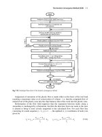
ability, as they are typically based on the data flow diagrams approach principle. A
standard problem solution in the SPSS Clementine system is shown on Figure 4; it
is a documentation of a chosen solution rather than a solution guide.
Fig. 4. Data flow principle in SPSS Clementine
3 Some data mining patterns
We have already developed some archetypical DM patterns. For their formal repre-

sentation the J.O. Coplien Pattern Formalization Form has been used (Coplien and
Zhao (2005), Coplien (1996), p 8). This form consists of the following elements:
Context, Problem, Forces, Solutions and Resulting context.
A pattern is applicable within a Context (description of the world) and creates a
Resulting Context, as the application of the Pattern will change the state space.
Problem describes what produces the uncomfortable feeling in a certain situation.
Forces are keys for pattern understanding. Each force will yield a quality critereon
for any solution, and as forces can be (and generally are) conflicting, the relative
importance of forces will drive a good solution into certain areas of the solution
A Pattern Based Data Mining Approach 331
space, hence their name. In many contexts, for instance, the relative importance of
the conflicting forces of economic, time and quality considerations will render a
particular solution a good or a bad compromise.
When a problem, forces as problem descriptors, are well understood, then a solu-
tion is most often easily evaluated. Understanding of a problem is crucial for finding
a solution. Patterns are functions that transform problems in a certain context into
solutions. Patterns are familiar and popular concepts, because they systematize re-
peatedly occuring solutions in nature. The solution, the pattern itself, resolves forces
in a problem and provides a good solution. On the other hand, a pattern is always a
compromise, it is not easy to recognize. Because it is a compromise it resolves some
forces, but may add to the context space new ones.
A pattern is best recognized through solving and generalizing real problems. The
quality and applicability of patterns may change over time as new forces gain rele-
vance or new solutions become available. The process of recognizing and deploying
patterns is continuous. For example, house building changed very much when con-
crete was invented.
3.1 The Condense Pattern: a popular DM pattern
The pattern is shown in the Coplien form is
1. Context: The collection of data is completed.
2. Problem: Data matrix is too large for efficient handling.

3. selected Forces:Efficiency of DM algorithms depends upon the number of cases
and variables. Irrelevant cases and variables will hamper learning capabilities of
DM algorithm. Leaving out a case or a variable may lead to errors and delete
special, but important cases.
4. Solution: Condense the data matrix
5. Resulting context: manageable data matrix with some information loss
The Condense pattern is a typical preprocessing pattern that has found diverse ap-
plications, for example on variables (by – for example – calculating a score, choosing
a representative variable or through clustering of variables), on cases (through sam-
pling, clustering with subsequent use of centers only, etc) or in transformation of
continuous variables (e.g. through equal width binning, equal frequency binning).
3.2 The Divide et Impera Pattern
A second pattern which is widely used in data mining is Divide et Impera. It can also
be described in the Coplien pattern form:
1. Context: A data mining problem is too large/complicated to be solved in one
step.
2. Problem: Structuring of the task
332 Boris Delibaši
´
c, Kathrin Kirchner and Johannes Ruhland
3. Forces: It is not possible to subdivide the problem, there are many strongly in-
terrelated facets influencing the problem. The sheer combination of subproblem
solutions may be grossly suboptimal. Subproblems may have very different rel-
evance for the global problem. Complexity of a generated subproblem may be
grossly out of proportion to its relevance. Solution: Divide the problem into sub-
problems that are more easily solved (and quite often structurally similar to the
original one) and build the solution to the complete problem as a combination.
4. Resulting context: a set of smaller problems, more palatable to solution
- It is possible that the problem structure is bad or the effort has not
been reduced in sum.

- The effort has not been reduced in sum.
The Divide et Impera pattern can be used for problem structuring where the prob-
lem is too complex to solve it in one step. It is found as a typical meta heuristic in
many algorithms such as decision trees or divisive clustering. Other application ar-
eas, which also vouch for its broad applicability, are segmented marketing (if an
across-the-board marketing strategy is not feasible, try to form homogeneous seg-
ments and cater to their needs), or the division of labor within divisional organiza-
tions.
3.3 More patterns in data mining
We have already identified a lot of other patterns in the field of data mining. Some of
them are:
• Combine voting(with boosting, bagging, stacking, etc. as corresponding algo-
rithms),
• Training / Retraining (supervised mining, etc.),
• Solution analysis,
• Categorization and
• Normalization
This list is in no way closed. Every area of human interest has its characteristic
patterns. However, there is not an infinite number of patterns, but always a limited
one. Collecting them and making them available for users gives the users the pos-
sibility to model the DM process, but also to understand the DM process through
patterns.
4 Summary and outlook
Pattern based data-mining offers some attractive features
1. The algorithm creators and the algortihm users have different interests and dif-
ferent need. These sides often don’t understand each others needs and, quite
often, do not need to know about specific details relevant to the other side. A
pattern is something that is understandable to all people.