Data Analysis Machine Learning and Applications Episode 2 Part 4 doc

A Pattern Based Data Mining Approach 333
2. Science converges. Concepts in one area of science is applicable in another area.
Patterns support these processes. This potential is comparable to the promises of
Systems Theory.
3. Decision for a specific algorithm can be postponed to later stages. A solution
path as a whole will be sketched through patterns and algorithms need only be
filled in immediately prior to processing. Using differnet algorithms in places
will not invalidate the solution path, creating “late binding” at the algorithm
level.
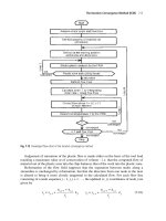
Current Data Mining applications occasionally provide the user with first traces
of pattern based DM. Figure 5 shows the example of Bagging of Classifiers within
the TANAGRA project and its graphical user interface (Rakotomalala (2004)). Bag-
ging cannot be described with a pure data flow paradigm, rather a nesting of a clas-
sifier pattern within the bagging pattern is needed. This nested structure will then be
pipelined with pre- and postprocessing patterns.
Fig. 5. Screenshot of Tanagra Software
Further steps in our project are to
• collect a list of patterns which are useful in the whole knowledge dis-
covery process and data mining (list will be open-ended).
• integrate these patterns into data mining software to help design ad-hoc
algorithms, choose an existing one or have guidance in the data mining
process.
• develop a software prototype with our pattern and make experiments
with users: how it works and what are the benefits.
334 Boris Delibaši
´
c, Kathrin Kirchner and Johannes Ruhland
References
ALEXANDER, C. (1979): The Timeless Way of Building, Oxford University Press.
ALEXANDER, C. (2002a): The Nature of Order Book 1: The Phenomenon of Life, The Center
for Environmental Structure, Berkeley, California.

ALEXANDER, C. (2002b): The Nature of Order Book 2: The Process of Creating Life, The
Center for Environmental Structure, Berkeley, California.
CHAPMAN, P., CLINTON, J., KERBER, R., KHABAZA, T., REINARTZ, T., SHEARER,
C. and WIRTH, R. (2000): CRISP-DM 1.0. Step-by-step data mining guide, www.crisp-
dm.org.
COPLIEN, J.O.(1996): Software Patterns, SIGS Books & Multimedia.
COPLIEN, J.O. and ZHAO, L. (2005): Toward a General Formal Foundation of Design -
Symmetry and Broken Symmetry, Brussels: VUB Press.
ECKERT, C. and CLARKSON, J. (2005): Design Process Improvement: a review of current
practice, Springer Verlag London.
FAYYAD, U.M., PIATETSKY-SHAPIRO, G. and UTHURUSAMY, R. (Ed.) (1996): Ad-
vances in Knowledge Discovery and Data Mining, MIT Press.
GAMMA, E., HELM, R., JOHNSON, R. and VLISSIDES, J. (1995): Design Patterns. Ele-
ments of Reusable Object-Oriented Software, Addison-Wesley.
HIPPNER, H., MERZENICH, M. and STOLZ, C. (2002): Data Mining: Einsatzpotentiale und
Anwendungspraxis in deutschen Unternehmen, In: WILDE, K.D.: Data Mining Studie,
absatzwirtschaft.
RAKOTOMALALA, R. (2004): Tanagra – A free data mining software for research and edu-
cation, www.eric.univ-lyon2.fr/∼rico/tanagra/.
WITTEN, I.H. and FRANK, E. (2005): Data Mining: Practical machine learning tools and
techniques, Morgan Kaufmann, San Francisco.
A Procedure to Estimate Relations in a Balanced
Scorecard
Veit Köppen
1
, Henner Graubitz
2
, Hans-K. Arndt
2
and Hans-J. Lenz

1
1
Institut für Produktion, Wirtschaftsinformatik und Operations Research
Freie Universität Berlin, Germany
{koeppen, hjlenz}@wiwiss.fu-berlin.de
2
Arbeitsgruppe Wirtschaftsinformatik - Managementinformationssysteme
Otto-von-Guericke-Universität Magdeburg, Germany
{graubitz, arndt}@iti.cs.uni-magdeburg.de
Abstract. A Balanced Scorecard is more than a business model because it moves perfor-
mance measurement to performance management. It consists of performance indicators which
are inter-related. Some relations are hard to find, like soft skills. We propose a procedure to
fully specify these relations. Three types of relationships are considered. For the function types
inverse functions exist. Each equation can be solved uniquely for variables at the right hand
side. By generating noisy data in a Monte Carlo simulation, we can specify function type and
estimate the related parameters. An example illustrates our procedure and the corresponding
results.
1 Related work
Indicator systems are appropriate instruments to define business targets and to mea-
sure management indicators together. Such a system should not be just a system of
hard indicators; it should be used as a system with control in which one can bring
hard indicators and management visions together.
In the beginning of the 90’s Johnson and Kaplan (1987) published the idea how
to bring a company’s strategy and used indicators together. This system, also known
as Balanced Scorecards (BSC), is developed until now.
The relationships between those indicators are hard to find. According to Marr
(2004), companies understand better their business if they visualise relations between
available indicators. However, some indicators influence each other in cause and
effect relations which increases the validity of these indicators. Unusually, compared
to a study of Ittner et al (2003) and Marr (2004) 46% of questioned companies do

not or are not able to visualise cause-and-effect relations of indicators.
Several approaches try to solve the existing shortcomings.
A possible way to model fuzzy relations in a BSC is described in Nissen (2006).
Nevertheless, this leads to restrictions in the variable domains.
364 Veit Köppen et al.
Blumenberg et al (2006) concentrate on Bayesian Belief Networks (BBN) and
try to predict value chain figures and enhanced corporate learning. The weakness of
this prediction method is that it does not contain any loops which BSCs may contain.
Loops within BSCs must be removed if BBN are used to predict causes and effects
in BSCs.
Banker et al (2004) suggest calculating trade-offs between indicators. The weak-
ness of this solution is that they concentrate on one financial and three nonfinancial
performance indicators and try to derive management decisions.
A totally different way of predicting relations in BSCs is the usage of system
dynamics. System Dynamics is usually used to simulate complex dynamic systems
(Forrester (1961)). Various publications exist of how to combine these indicators
with dynamics systems to predict economic scenarios in a company, e.g. Akkermans
et al (2002). In contrast to these approaches we concentrate on existing performance
indicators and try to predict relationships between these indicators instead of pre-
dicting economic scenarios. It is similar to the methods of system identification. In
contrast, our approach calculates in a more flexible way all models within the de-
scribed model classes (see section 3).
2 Balanced scorecards
”If you can’t measure it, you can’t manage it” (Kaplan and Norton (1996), p. 21).
With this sentence the BSC inventors Kaplan and Norton made a statement which
describes a common problem in the industry: you can not manage a company if
you don’t have performance indicators to manage and control your company.Kaplan
and Norton presented the BSC – a management tool for bringing the current state
of the business and the strategy of the company together. It is a result of previous
indicator systems. Nevertheless, a BSC is more than a business system (Friedag &

Schmidt 2004). Kaplan & Norton (2004) emphasise this in their further development
of Strategy Maps.
However, what are these performance indicators and how can you measure it.
PreiSSner (2002) divides the functionality of indicators into four topics: operational-
isation (”indicators should be able to reach your goal”), animation (”a frequent mea-
surement gives you the possibility to recognise important changes”), demand (”it can
be used as control input”) and control (”it can be used to control the actual value”).
Nonetheless, we understand an indicator as defined in (Lachnit 1979).
But before a decision is made which indicator is added to the BSC and the corre-
sponding perspective the importance of the indicator has to be evaluated. Kaplan &
Norton divide indicators additionally into hard and soft, short and long-term objec-
tives. They also consider cause and effect relations. The three main aspects are: 1. All
indicators that do not make sense are not worthwhile being included into a BSC; 2.
While building a BSC, a company should differentiate between performance and re-
sult indicators; 3. All non-monetary values should influence monetary values. Based
on these indicators we are now able to build up a complete system of indicators which
A Procedure to Estimate Relations in a Balanced Scorecard 365
turns into or influences each other and seeks a measurement for one of the follow-
ing four perspectives: (1) Financial Perspective to reflect the financial performance
like the return on investment; (2) Customer Perspective to summarize all indicators
of the customer/company relationships; (3) Business Process Perspective to give an
overview about key business processes; (4) Learning and Growth Perspective which
measures the company’s learning curve.
Financial
Profitability
Customer
Lower Costs Increase Revenue
More customers
Lowest Prices
Internal

Improve
Turnaround
Time
OnŦtime flights
Align
Ground
Crews
Learning
Fig. 1. BSC Example of a domestic airline
By splitting a company into four different views the management of a company
gets the chance of a quick overview. The management can focus on its strategic goal
and is able to react in time. They are able to connect qualitative performance indi-
cators with one or all business indicators. Moreover the construction of an adequate
equation system might be impossible.
Nevertheless the relations between indicators should be elaborated and an approx-
imation of the relations of these indicators should be considered. In this case mul-
tivariate density estimation is an appropriate tool for modeling the relations of the
business. Figure 1 shows a simple BSC of an airline company. Profitability is the
main figure of interest but additionally seven more variables are useful for manag-
ing the company. Each arc visualizes the cause and effect relations. This example is
taken from "The Balanced Scorecard Institute"
1
.
1
www.balancedscorecard.org
366 Veit Köppen et al.
3 Model
To quantify the relationships in a given data set different methods for parameter esti-
mation are used. Measurement errors within the data set are allowed, but these errors
are assumed to have a mean value of zero. For each indicator within the data set no

missing data is assumed. To quantify the relationships correctly it is further assumed
that intermediate results are included in the data set. Otherwise the relationships will
not be covered. Heteroscedasticity as well as autocorrelations of the data is not con-
sidered.
3.1 Relationships, estimations and algorithm
In our procedure three different types of relationships are investigated. The first two
function types are unknown because the operators linking the variables are unknown:
z = f (x,y)=x⊗y (1)
where ⊗ represent an addition or a multiplication operator. The third type includes a
parametric type of real valued function:
y = f
T
(x)=
⎧
⎪
⎨
⎪
⎩
px≤ a
c
1+e
−d·(x−g)
+ ha< x ≤ b
qx> b
(2)
with T =(abcdgh) and p =
c
1+e
−d·(a−g)
+h and q =

c
1+e
−d·(b−g)
+h. Note, that all three
function types are assumed to be separable, i.e. uniquely solvable for x or y in 1
and x in 2. Thus forward and backward calculations in the system of indicators are
possible. As a data set is tested independently with respect to the described function
types a
ˆ
Sidàk correction has to be applied (cf. Abdi (2007)).
Additive relationships between three indicators (Y = X
1
+ X
2
) are detected via
multiple regression. The model is:
Y = E
0
+ E
1
·X
1
+ E
2
·X
2
+ u (3)
where u ∼ N(0, V
2
). The relationship is accepted if level of significance of all ex-

planatory variables is high and E
0
= 0, E
1
= 1 and E
2
= 1. The multiplicative rela-
tionship Y = X
1
·X
2
is detected by the regression model:
Y = E
0
+ E
1
·Z + u with Z = X
1
·X
2
,u ∼N(0,V
2
). (4)
The relationship is accepted if the level of significance of the explanatory variable
is high and E
0
= 0andE
1
= 1. The nonlinear relationship between two indicators
according to equation 2 is detected by parameter estimation based on nonlinear re-

gression:
Y =
c
1+ e
−d·(X−g)
+ h + u ∀a < x ≤ b;u ∼N(0,V
2
). (5)
A Procedure to Estimate Relations in a Balanced Scorecard 367
In a first step the indicators are extracted from a business database, files or
tools like excel spreadsheets. The number of extracted indicators is denoted by n.
In the second step all possible relationships have to be evaluated. For the multiple
regression scenario
n!
3!·(n−3)!
cases are relevant. Testing multiplicative relationships
demands
n!
2·(n−3)!
test cases. The nonlinear regression needs to be performed
n!
(n−2)!
times. All regressions are performed in R. The univariate and the multivariate linear
regression are performed with the
lm
function from the R-base stats package. The
nonlinear regression is fitted by the
nls
function in the stats package and the level of
significance is evaluated. If additionally the estimated parameter values are in given

boundaries the relationship is accepted.
The pseudo code of the the complete environment is given in algorithm 3.1.
Algorithm 1 Estimation Procedure
Require: data matrix data[M
t×n
]witht observations for n indicators
significance level, boundaries for parameter
Ensure: detected relationships between indicators
1: for i =1ton −2 AND j = i +1 ton − 1 AND k = j +1 ton do
2: estimation by lm(data[,i] data[,j] + data[,k])
3: if significant AND parameter estimates within boundaries then
4: Relationship ”Addition” found
5: end if
6: end for
7: for i =1ton AND j =1ton − 1 AND k = j +1ton do
8: if i!=jANDi!=k then
9: set Z := data[,j] · data[,k]
10: estimation by lm(data[,i] Z)
11: if significant AND parameter estimates within boundaries then
12: Relationship ”Multiplication” found
13: end if
14: end if
15: end for
16: for i =1ton AND j =1ton do
17: if i!=jthen
18: estimation by nls(data[,j] c/(1+exp(-d+g*data[,i])) + h)
19: if significant then
20: ”Nonlinear Relationship” found
21: end if
22: end if

23: end for
4 Case study
For our case study we create an artificial model with 16 indicators and 12 relation-
ships, see Fig. 2. It includes typical cases of the real world.
368 Veit Köppen et al.
IndicatorPlus 1
IndicatorPlus 2
Indicator 1 Indicator 3 Indicator 4Indicator 2
IndicatorExp 2
exp
IndicatorPlus 3
x
IndicatorMultiply 3
IndicatorPlus 4
+
x
IndicatorMultiply 4
exp
IndicatorExp1
IndicatorExp 4
exp
x
IndicatorMultiply 1
exp
IndicatorExp 3
x
IndicatorMultiply 2
+
+
+

Fig. 2. Artificial Example
Indicators 1-4 are independently and randomly distributed. In Fig. 2 they are dis-
played in grey and represent the basic input for the simulated BSC system. All other
indicators are either functional dependent on two indicators related by an addition or
multiplication or functional dependent on an indicator according to equation 2. Some
of these indicators effect other quantities or represent leaf nodes in the BSC model
graph, cf. Fig. 2. Based on the fact that indicators may not be precisely measured
we add noise to some indicators, see Tab. 1. Note, that IndicatorPlus4 has a skewed
added noise whereas the remaining added noise is symmetrical.
In our case study we hide all given relationships and try to identify them, cf.
section 3.
Table 1. Indicator Distributions and Noise
Indicator Distribution Indicator added Noise Indicator Noise
Indicator1 N(100, 10
2
) IndicatorPlus1 N(0,1) IndicatorExp1 N(0, 1)
Indicator2 N(40, 2
2
) IndicatorPlus4 E(1) −1 IndicatorExp4 U(−1,1)
Indicator3 U(−10,10) IndicatorMultiply1 N(0, 1)
Indicator4 E(2) IndicatorMultiply4 U(−1,1)
5 Results
The case study runs in three different stages: with 1k, 10k, and 100k randomly dis-
tributed data. The results are similar and can be classified into four cases: (1) if a
A Procedure to Estimate Relations in a Balanced Scorecard 369
relation exists and it was found (displayed black in Fig. 3), (2) if a relation was found
but does not exist (displayed with a pattern in Fig. 3) (error of the second kind), (3)
if no relation was found but one exists in the model (displayed white in Fig. 3) (error
of the first kind), and (4) if no relation exists and no one was found. Additionally the
results have been split according to the operator class (see Tab. 2).

Table 2. Identification Results
Observations 1k 10k 100k
+*Exp+*Exp+*Exp
(2) 032705480249
(3)
103103103
560 1680 240 560 1680 240 560 1680 240
Hence, Tab. 2 shows that the results for all experiments are similar for the oper-
ators addition and multiplication. For non-linear regression, relationships could not
be discovered properly.
The additive relation of IndicatorPlus4 was the only non-detective relation, see
observation (3) in Tab. 2. This is caused by the fact that the indicator has an added
noise which is skewed. In such a case the identification is not possible.
IndicatorPlus 1
IndicatorPlus 2
Indicator 1 Indicator 3 Indicator 4Indicator 2
IndicatorExp 2
IndicatorPlus 3
IndicatorMultiply 3
IndicatorPlus 4
+
IndicatorMultiply 4
exp
IndicatorExp1
IndicatorExp 4
exp
IndicatorMultiply 1
exp
IndicatorExp 3
IndicatorMultiply 2

x
x
x
+
x
x
+
+
x
exp
Fig. 3. Results of the Artificial Example for 100k observations
370 Veit Köppen et al.
6 Conclusion and outlook
Traditional regression analysis allows estimating the cause and effect dependencies
within a profit seeking organization. Univariate and multivariate linear regression
exhibit the best results whereas skewed noise in the variables destroys the possibility
to detect these relationships.
Non-linear regression has a high error output due to the fact that optimization
has to be applied and starting values are not always at hand. The results from the
non-linear regression should only be carefully taken into account.
In future work we try to improve our results while removing indicators for which
we calculate a nearly 100% secure relationship. Additionally we plan to work on real
data which also includes the possibility of missing data for indicators. Research aims
at creating a company’s BSC with relevant business figures while looking only at a
company’s indicator system.
References
ABDI, H. (2007): Bonferroni and Sidak corrections for multiple comparisons. In: N.J. Salkind
(Ed.): Encyclopedia of Measurement and Statistics. Thousand Oaks (CA): Sage: 103–
107.
AKKERMANS, H. and VAN OORSCHOT, KIM (2002): Developing a balanced scorecard

with system dynamics in Proceeding of 2002 International System Dynamics Conference.
BANKER, R. D. and Chang, H. and JANAKIRAMAN, S. N. and KONSTANS, C. (2004): A
balanced scorecard analysis of performance metrics. in European Journal of Operational
Research 154(2): 423–436.
BLUMENBERG, STEFAN A. and HINZ, DANIEL J. (2006): Enhancing the Prognostic
Power of IT Balanced Scorecards with Bayesian Belief Networks. In HICSS ’06: Pro-
ceedings of the 39th Annual Hawaii International Conference on System Sciences IEEE
Computer Society, Washington, DC, USA
FORRESTER, J. W. (1961). Industrial Dynamics Waltham, MA: Pegasus Communications.
FRIEDAG, H.R. and SCHMIDT, W. (2004): Balanced Scorecard. 2nd edition. Haufe,
Planegg.
ITTNER, C.D. and LARCKER, D.F. and RANDALL, T. (2003): Performance implications of
strategic performance measurement in financial service firms". Accounting Organization
and Society, 2nd edition. Haufe, Planegg.
JOHNSON, T.H. and KAPLAN, R.S. (1987): Relevance lost: the rise and fall of management
accounting . Harvard Business Press, Boston.
KAPLAN, R.S. and NORTON, D.P. (1996): The Balanced Scorecard. Translating Strategy
Into Action. Harvard Business School Press, Harvard.
KÖPPEN, V. and LENZ, H J. (2006): A comparison between probabilistic and possibilistic
models for data validation. In: Rizzi, A. & Vichi, M. (Eds.) Compstat 2006
˝
U Proceedings
in Computational Statistics , Springer, Rome.
LACHNIT, L. (1979): Systemorientierte Jahresabschlussanalyse. Betriebswirtschaftlicher
Verlag Dr. Th. Gabler KG, Wiesbaden.
MARR, B. (2004): Business Performance Measurement: Current State of the Art. Cranfield
University, School of Management, Centre for Business Performance.
A Procedure to Estimate Relations in a Balanced Scorecard 371
NISSEN, V. (2006): Modelling Corporate Strategy with the Fuzzy Balanced Scorecard. In:
Hüllermeier, E. et al. (Eds.): Proceedings Symposium on Fuzzy Systems in Computer

Science FSCS 2006: 121– 138, Magdeburg.
PREISSNER, A. (2002): Balanced Scorecard in Vertrieb und Marketing: Planung und Kon-
trolle mit Kennzahlen, 2nd ed. Hanser Verlag, München, Wien
Benchmarking Open-Source Tree Learners in
R/RWeka
Michael Schauerhuber
1
, Achim Zeileis
1
,DavidMeyer
2
, Kurt Hornik
1
1
Department of Statistics and Mathematics
Wirtschaftsuniversität Wien
1090 Wien, Austria
2
Institute for Management Information Systems
Wirtschaftsuniversität Wien
1090 Wien, Austria
{Michael.Schauerhuber, Achim.Zeileis, Kurt.Hornik}@wu-wien.ac.at
Abstract. The two most popular classification tree algorithms in machine learning and statis-
tics — C4.5 and CART — are compared in a benchmark experiment together with two other
more recent constant-fit tree learners from the statistics literature (QUEST, conditional infer-
ence trees). The study assesses both misclassification error and model complexity on bootstrap
replications of 18 different benchmark datasets. It is carried out in the
R system for statistical
computing, made possible by means of the RWeka package which interfaces
R to the open-

source machine learning toolbox Weka. Both algorithms are found to be competitive in terms
of misclassification error—with the performance difference clearly varying across data sets.
However, C4.5 tends to grow larger and thus more complex trees.
1 Introduction
Due to their intuitive interpretability, tree-based learners are a popular tool in data
mining for solving classification and regression problems. Traditionally, practition-
ers with a machine learning background use the C4.5 algorithm (Quinlan, 1993)
while statisticians prefer CART (Breiman, Friedman, Olshen and Stone, 1984). One
important reason for this is that free reference implementations have not been easily
available within an integrated computing environment. RPart, an open-source im-
plementation of CART, has been available for some time in the
S/R package rpart
(Therneau and Atkinson, 1997) while the open-source implementation J4.8 for C4.5
became available more recently in the Weka machine learning package (Witten and
Frank, 2005) and is now accessible from within
R by means of the RWeka package
(Hornik, Zeileis, Hothorn and Buchta, 2007). With these software tools available,
the algorithms can be easily compared and benchmarked on the same computing
platform: the
R system for statistical computing (R Development Core Team 2006).
The principal concern of this contribution is to provide a neutral and unprejudiced
390 Michael Schauerhuber et al.
review, especially taking into account classical beliefs (or preconceptions) about per-
formance differences between C4.5 and CART and heuristics for the choice of hyper-
parameters. With this in mind, we carry out a benchmark comparison, including dif-
ferent strategies for hyper-parameter tuning as well as two further constant-fittree
models—QUEST (Loh and Shih, 1997) and conditional inference trees (Hothorn,
Hornik and Zeileis, 2006). The learners are compared with respect to misclassifica-
tion error and model complexity on each of 18 different benchmarking data sets by
means of simultaneous confidence intervals (adjusted for multiple testing). Across

data sets, the performance is aggregated by consensus rankings.
2 Design of the benchmark experiment
The simulation study includes a total of six tree-based methods for classification.
All learners were trained and tested in the framework of Hothorn, Leisch, Zeileis
and Hornik (2005) based on 500 bootstrap samples for each of 18 data sets. All
algorithms are trained on each bootstrap sample and evaluated on the remaining out-
of-bag observations. Misclassification rates are used as predictive performance mea-
sures, while model complexity requirements of the algorithms under study are mea-
sured by the number of estimated parameters (number of splits plus number of leafs).
Performance and model complexity distributions are assessed for each algorithm on
each of the datasets. In our setting, this results in 108 performance distributions (6
algorithms on 18 data sets), each of size 500. For comparison on each individual
data set, simultaneous pairwise confidence intervals (Tukey all-pair comparisons)
are used. For aggregating the pairwise dominance relations across data sets, median
linear order consensus rankings are employed following Hornik and Meyer (2007). A
brief description of the algorithms and their corresponding implementation is given
below.
CART/RPart: Classification and regression trees (CART, Breiman et al., 1984) is the
classical recursive partitioning algorithm which is still the most widely used in
the statistics community. Here, we employ the open-source reference implemen-
tation of Therneau and Atkinson (1997) provided in the
R package rpart.For
determining the tree size, cost-complexity pruning is typically adopted: either by
using a 0- or 1-standard-errors rule. The former chooses the complexity param-
eter associated with the smallest prediction error in cross-validation (RPart0),
whereas the latter chooses the highest complexity parameter which is within 1
standard error of the best solution (RPart1).
C4.5/J4.8: C4.5 (Quinlan, 1993) is the predominantly used decision tree algorithm
in the machine learning community. Although source code implementing C4.5
is available in Quinlan (1993), it is not published under an open-source license.

Therefore, the
Java implementation of C4.5 (revision 8), called J4.8, in Weka
is the de-facto open-source reference implementation. For determining the tree
size, a heuristic confidence threshold C is typically used which is by default
set to C = 0.25 (as recommended in Witten and Frank, 2005). To evaluate the
Benchmarking Open-Source Tree Learners in R/RWeka 391
Table 1. Artificial [∗] and non artificial benchmarking data sets
Data set # of obs. # of cat. inputs # of num. inputs
breast cancer 699 9 -
chess 3196 36 -
circle ∗ 1000 - 2
credit 690 - 24
heart 303 8 5
hepatitis 155 13 6
house votes 84 435 16 -
ionosphere 351 1 32
liver 345 - 6
Pima Indians diabetes 768 - 8
promotergene 106 57 -
ringnorm ∗ 1000 - 20
sonar 208 - 60
spirals ∗ 1000 - 2
threenorm ∗ 1000 - 20
tictactoe 958 9 -
titanic 2201 3 -
twonorm ∗ 1000 - 20
influence of this parameter, we compare the default J4.8 algorithm with a tuned
version where C and the minimal leaf size M (default: M = 2) are chosen by
cross-validation (J4.8(cv)). A full grid search for C = 0.01,0.05,0.1, ,0.5 and
M = 2,3, ,10,15, 20 is used in the cross-validation.

QUEST: Quick, unbiased and efficient statistical trees are a class of decision trees
suggested by Loh and Shih (1997) in the statistical literature. QUEST popular-
ized the concept of unbiased recursive partitioning, i.e., avoiding the variable se-
lection bias of exhaustive search algorithms (such as CART and C4.5). A binary
implementation is available from
/>html
and interfaced in the R package LohTools which is available from the au-
thors upon request.
CTree: Conditional inference trees (Hothorn et al., 2006) are a framework of un-
biased recursive partitioning based on permutation tests (i.e., conditional infer-
ence) and applicable to inputs and outputs measured at arbitrary scale. An open-
source implementation is provided in the
R package party.
The benchmarking datasets shown in Table 1 were taken from the popular UCI
repository of machine learning databases (Newman, Hettich, Blake and Merz, 1998)
as provided in the
R package mlbench.
392 Michael Schauerhuber et al.
3 Results of the benchmark experiment
3.1 Results on individual datasets: Pairwise confidence intervals
Here, we exemplify—using the well-known Pima Indians diabetes and breast cancer
data sets—how the tree algorithms are assessed on a single data set. Simultaneous
confidence intervals are computed for all 15 pairwise comparisons of the 6 learners.
The resulting dominance relations are used as the input for the aggregation analyses
in Section 3.2.
Pima Indians Diabetes: Misclassification
Ŧ2.5 Ŧ1.5 Ŧ0.5 0.0 0.5
CTree Ŧ QUEST
CTree Ŧ RPart1
QUEST Ŧ RPart1

CTree Ŧ RPart0
QUEST Ŧ RPart0
RPart1 Ŧ RPart0
CTree Ŧ J4.8(cv)
QUEST Ŧ J4.8(cv)
RPart1 Ŧ J4.8(cv)
RPart0 Ŧ J4.8(cv)
CTree Ŧ J4.8
QUEST Ŧ J4.8
RPart1 Ŧ J4.8
RPart0 Ŧ J4.8
J4.8(cv) Ŧ J4.8
(
(
(
(
(
(
(
(
(
(
(
(
(
(
(
)
)
)

)
)
)
)
)
)
)
)
)
)
)
)
Pima Indians Diabetes: Misclassification
Misclassification difference (in percent)
Pima Indians Diabetes: Complexity
Ŧ80 Ŧ60 Ŧ40 Ŧ20 0 20
CTree Ŧ QUEST
CTree Ŧ RPart1
QUEST Ŧ RPart1
CTree Ŧ RPart0
QUEST Ŧ RPart0
RPart1 Ŧ RPart0
CTree Ŧ J4.8(cv)
QUEST Ŧ J4.8(cv)
RPart1 Ŧ J4.8(cv)
RPart0 Ŧ J4.8(cv)
CTree Ŧ J4.8
QUEST Ŧ J4.8
RPart1 Ŧ J4.8
RPart0 Ŧ J4.8

J4.8(cv) Ŧ J4.8
(
(
(
(
(
(
(
(
(
(
(
(
(
(
(
)
)
)
)
)
)
)
)
)
)
)
)
)
)

)
Pima Indians Diabetes: Complexity
Complexity difference
Breast Cancer: Misclassification
Ŧ1.0 Ŧ0.5 0.0 0.5 1.0
CTree Ŧ QUEST
CTree Ŧ RPart1
QUEST Ŧ RPart1
CTree Ŧ RPart0
QUEST Ŧ RPart0
RPart1 Ŧ RPart0
CTree Ŧ J4.8(cv)
QUEST Ŧ J4.8(cv)
RPart1 Ŧ J4.8(cv)
RPart0 Ŧ J4.8(cv)
CTree Ŧ J4.8
QUEST Ŧ J4.8
RPart1 Ŧ J4.8
RPart0 Ŧ J4.8
J4.8(cv) Ŧ J4.8
(
(
(
(
(
(
(
(
(
(

(
(
(
(
(
)
)
)
)
)
)
)
)
)
)
)
)
)
)
)
Breast Cancer: Misclassification
Misclassification difference (in percent)
Breast Cancer: Complexity
Ŧ15 Ŧ10 Ŧ50 510
CTree Ŧ QUEST
CTree Ŧ RPart1
QUEST Ŧ RPart1
CTree Ŧ RPart0
QUEST Ŧ RPart0
RPart1 Ŧ RPart0

CTree Ŧ J4.8(cv)
QUEST Ŧ J4.8(cv)
RPart1 Ŧ J4.8(cv)
RPart0 Ŧ J4.8(cv)
CTree Ŧ J4.8
QUEST Ŧ J4.8
RPart1 Ŧ J4.8
RPart0 Ŧ J4.8
J4.8(cv) Ŧ J4.8
(
(
(
(
(
(
(
(
(
(
(
(
(
(
(
)
)
)
)
)
)

)
)
)
)
)
)
)
)
)
Breast Cancer: Complexity
Complexity difference
Fig. 1. Simultaneous confidence intervals of pairwise performance differences (left: misclas-
sification, right: complexity) for Pima Indians diabetes (top) and breast cancer (bottom) data.
As can be seen from the performance plots for Pima Indian diabetes in Figure 1,
standard J4.8 is outperformed (in terms of misclassification as well as model com-
plexity) by the other tree learners. All other algorithm comparisons indicate equal
predictive performances, except for the comparison of RPart0 and J4.8(cv), where
the former learner performs slightly better than the latter. On this particular dataset
tuning enhances the predictive performance of J4.8, while the misclassification rates
of the differently tuned RPart versions are not subject to significant changes. In terms
of model complexity J4.8(cv) produces larger trees than the other learners. Looking
Fig. 2. Distribution of J4.8(cv) parameters obtained through cross validation on Pima Indians
diabetes and breast cancer data sets.
at the breast cancer data yields a rather different picture: Both RPart versions are
outperformed by J4.8 or its tuned alternative in terms of predictive accuracy. Similar
to Pima Indians diabetes, J4.8 and J4.8(cv) tend to build significantly larger trees
than RPart. On this dataset, CTree has a slight advantage over all other algorithms
except J4.8 in terms of predictive accuracy. For J4.8 as well as RPart, tuning does
not promise to increase predictive accuracy significantly. A closer look at the dif-
fering behavior of J4.8(cv) under cross validation for both data sets is provided in

Figure 2. In contrast to the breast cancer example, the results based on the Pima
Indians diabetes dataset (on which tuning of J4.8 caused a significant performance
increase) show a considerable difference in choice of parameters. The multiple infer-
ence results gained from all datasets considered in this simulation experiment (just
like the results derived from the two datasets above) form the basis on which further
aggregation analyses of Section 3.2 are built upon.
3.2 Results across data sets: Consensus Rankings
Having 18×6 = 108 performance distributions of the 6 different learners applied to
18 bootstrap data settings at hand, aggregation methods can do a great favor to al-
low for summarizing and comparing algorithmic performance. The underlying dom-
inance relations derived from the multiple testing are summarized by simple sums in
Table 2 and by the corresponding median linear order rankings in Table 3. In Table 2,
rows refer to winners, while columns denote the losers. For example J4.8 managed
to outperform QUEST on 11 datasets and 4 times vice versa, i.e., on the remaining 3
datasets, J4.8 and QUEST perform equally well.
The median linear order for misclassification reported in Table 3 suggests that
tuning of J4.8 instead of using the heuristic approach is worth the effort. A similar
Benchmarking Open-Source Tree Learners in R/RWeka 393
394 Michael Schauerhuber et al.
Table 2. Summary of predictive performance dominance relations across all 18 datasets based
on misclassification rates and model complexity (columns refer to losers, rows are winners).
Misclassification
J4.8 J4.8(cv) RPart0 RPart1 QUEST CTree

J4.8 029911839
J4.8(cv)
408911941
RPart0
560710735
RPart1

64108625
QUEST
42250720
CTree
76789037

26 20 27 38 49 37
Complexity J4.8 J4.8(cv) RPart0 RPart1 QUEST CTree

J4.8 0100203
J4.8(cv)
17 0 0 0 5 3 25
RPart0
18 18 0 0 13 15 64
RPart1
18 18 16 0 14 15 81
QUEST
15 13 5 4 0 10 47
CTree
18 14 3 2 8 0 45

86 64 24 6 42 43
Table 3. Median linear order consensus rankings for algorithm performance
Misclassification Complexity
1 J4.8(cv) RPart1
2 J4.8 RPart0
3 RPart0 QUEST
4 CTree CTree
5 RPart1 J4.8(cv)
6 QUEST J4.8

conclusion can be made for the RPart versions. Here, the median linear order sug-
gests that the common one standard error rule performs worse. For both cases, the
underlying dominance relation figures of Table 2 catch our attention. Regarding the
first case, J4.8(cv) only dominates J4.8 in four of six data settings, in which a signifi-
cant test decision for performance differences could be made. In addition the remain-
ing 12 data settings yield equivalent performances. Therefore superiority of J4.8(cv)
above J4.8 is questionable. In contrast the superiority of RPart0 vs. RPart1 seems to
be more reliable but still the number of data settings producing tied results is high. A
comparison of the figures of CTree and the RPart versions confirms previous findings
(Hothorn et al., 2006) that CTree and RPart often perform equally well. The ques-
tion concerning the dominance relation between J4.8 and RPart cannot be answered
easily: Overall, the median linear order suggests that the J4.8 decision tree versions
are superior to the RPart tree learners in terms of predictive performance. But still,
looking at the underlying relations of the best performing versions of both algorithms
Benchmarking Open-Source Tree Learners in R/RWeka 395
(J4.8(cv) and RPart0) reveals that a confident decision concerning predictive supe-
riority cannot be made. The number of differences in favor of J4.8(cv) is only two
and no significant differences are reported on four data settings. A brief look at the
complexity ranking (Table 3) and the underlying complexity dominance relations
(Table 2, bottom) shows that J4.8 and its tuned version produce more complex trees
than the RPart algorithms. While analogous analyses of comparing J4.8 versions to
CTree do not indicate confident predictive performance differences, superiority of
the J4.8 versions versus QUEST in terms of predictive accuracy is evident.
0.0 0.1 0.2 0.3 0.4
024681012
medium confidence threshold (C)
medium minimal leaf size (M)
Fig. 3. Medians of the J4.8(cv) tuning parameter distributions for C and M
To aggregate the tuning results from J4.8(cv), Figure 3 depicts the median C
and M parameters chosen for each of the 18 parameter distributions. It confirms

the finding from the individual breast cancer and Pima Indians diabetes results (see
Figure 2) that the parameter chosen by cross-validation can be far off the default
values for C and M.
4 Discussion and further work
In this paper, we present results of a medium scale benchmark experiment with a
focus on popular open-source tree-based learners available in
R. With respect to
our two main objectives – performance differences between C4.5 and CART, and
heuristic choice of hyper-parameters – we can conclude: (1) The fully cross-validated
J4.8(cv) and RPart0 perform better than their heuristic counterparts J4.8 (with fixed
hyper-parameters) and RPart1 (employing a 1-standard-error rule). (2) In terms of
predictive performance, no support for the claims of (clear) superiority of either al-
gorithm can be found: J4.8(cv) and RPart0 lead to similar misclassification results,
however J4.8(cv) tends to grow larger trees. Overall, this suggests that many beliefs
396 Michael Schauerhuber et al.
or preconceptions about the classical tree algorithms should be (re-)assessed using
benchmark studies. Our contribution is only a first step in this direction and further
steps will require a larger study with additional datasets and learning algorithms.
References
BREIMAN, L., FRIEDMAN, J., OLSHEN, R. and STONE, C. (1984): Classification and
Regression Trees. Wadsworth, Belmont, CA, 1984.
HORNIK, K. and MEYER, D. (2007): Deriving Consensus Rankings from Benchmarking
Experiments In: Advances in Data Analysis (Proceedings of the 30th Annual Conference
of the Gesellschaft für Klassifikation e.V., March 8–10, 2006, Berlin), Decker, R., Lenz,
H J. (Eds.), Springer-Verlag, 163–170.
HORNIK, K., ZEILEIS, A., HOTHORN, T. and BUCHTA, C. (2007): RWeka:An
R Interface
to Weka.
R package version 0.3-2.
/>.

HOTHORN, T., HORNIK, K. and ZEILEIS, A. (2006): Unbiased Recursive Partitioning: A
Conditional Inference Framework. Journal of Computational and Graphical Statistics,
15(3), 651–674.
HOTHORN, T., LEISCH, F., ZEILEIS, A. and HORNIK, K. (2005): The Design and Analysis
of Benchmark Experiments. Journal of Computational and Graphical Statistics, 14(3),
675–699.
LOH, W. and SHIH, Y. (1997): Split Selection Methods for Classification Trees. Statistica
Sinica, 7, 815–840.
NEWMAN, D., HETTICH, S., BLAKE, C. and MERZ C. (1998): UCI Repository of Machine
Learning Databases.
/>.
QUINLAN, J. (1993): C4.5: Programs for Machine Learning. Morgan Kaufmann Publishers,
Inc., San Mateo, CA.
R DEVELOPMENT CORE TEAM (2006): R: A Language and Environment for Statistical
Computing.
R Foundation for Statistical Computing, Vienna, Austria. ISBN 3-900051-
07-0,
/>.
THERNEAU, T. and ATKINSON, E. (1997): An Introduction to Recursive Partitioning Using
the rpart Routine. Technical Report. Section of Biostatistics, Mayo Clinic, Rochester,
/>.
WITTEN, I., and FRANK, E. (2005): Data Mining: Practical Machine Learning Tools and
Techniques. Morgan Kaufmann, San Francisco, 2nd edition.
Combining Several SOM Approaches in Data Mining:
Application to ADSL Customer Behaviours Analysis
Francoise Fessant, Vincent Lemaire, Fabrice Clérot
R&D France Telecom, 22307 Lannion, France
{francoise.fessant,vincent.lemaire,fabrice.clerot}@orange-ftgroup.com
Abstract. The very rapid adoption of new applications by some segments of the ADSL cus-
tomers may have a strong impact on the quality of service delivered to all customers. This

makes the segmentation of ADSL customers according to their network usage a critical step
both for a better understanding of the market and for the prediction and dimensioning of the
network. Relying on a “bandwidth only" perspective to characterize network customer be-
haviour does not allow the discovery of usage patterns in terms of applications. In this paper,
we shall describe how data mining techniques applied to network measurement data can help
to extract some qualitative and quantitative knowledge.
1 Introduction
Broadband access for home users and small or medium business and especially
ADSL (Asymmetric Digital Subscriber Line) access is of vital importance for
telecommunication companies, since it allows them to leverage their copper infras-
tructure so as to offer new value-added broadband services to their customers. The
market for broadband access has several strong characteristics:
• there is a strong competition between the various actors,
• although the market is now very rapidly increasing, customer retention is impor-
tant because of high acquisition costs,
• new applications or services may be picked up very fast by some segments of the
customers and the behaviour of these applications or services may have a very
strong impact on the quality of service delivered to all customers (and not only
those using these new applications or services).
Two well-known examples of new applications or services with possibly very de-
manding requirements in term of bandwidth are peer-to-peer file exchange systems
and audio or video streaming.
The above characteristics explain the importance of an accurate understanding
of the customer behaviour and a better knowledge of the usage of broadband access.
The notion of “usage" is slowly shifting from a “bandwidth only" perspective to a
344 Francoise Fessant et al.
much broader perspective which involves the discovery of usage patterns in terms of
applications or services. The knowledge of such patterns is expected to give a much
better understanding of the market and to help anticipate the adoption of new services
or applications by some segments and allow the deployment of new resources before

the new usage effects hit all the customers.
Usage patterns are most often inferred from polls and interviews which allow an
in-depth understanding but are difficult to perform routinely, suffer from the small
size of the sampled population and cannot easily be extended to the whole popula-
tion or correlated with measurements (Anderson et al. (2002)). “Bandwidth only"
measurements are performed routinely on a very large scale by telecommunication
companies (Clement et al. (2002)) but do not allow much insight into the usage pat-
terns since the volumes generated by different applications can span many orders of
magnitude.
In this paper, we report another approach to the discovery of broadband cus-
tomers’ usage patterns by directly mining network measurement data. After a de-
scription of the data used in the study and their acquisition process, we explain the
main steps of the data mining process and we illustrate the ability of our approach to
give an accurate insight in terms of usages patterns of applications or services while
being highly scalable and deployable. We focus on two aspects of customers’ usages:
usage of types of applications and customers’ daily traffic; these analyses suppose to
observe the data at several levels of detail.
2 Network measurements and data description
2.1 Probes measurements
The network measurements are performed on ADSL customer traffic by means of
a proprietary network probe working at the SDH (Synchronous Digital Hierarchy)
level between the Broadband Access Server (BAS) and the Digital Subscriber Line
Access Multiplexer (DSLAM). This on-line probe allows to read and store all the
relevant fields of the ATM (Asynchronous Transfer Mode) cells and of the IP/TCP
headers. From now, 9 probes equip the network; they observe about 18000 customers
non-stop (a probe can observe about 2000 customers on a physical link). Once the
probe is in place, data collection is performed automatically. A detailed description
of the probe architecture can be found in (Francois (2002)).
2.2 Data description
For the study reported here, we gathered one month of data, on one site, for about two

thousand customers. The data give the volumes of data exchanged in the upstream
and downstream directions of twelve types of applications (web, peer-to-peer, ftp,
news, mail, db, control, games, streaming, chat, others and unknown) sampled for
each 6 minutes window for each customer. Most of the types of applications corre-
spond to a group of well-known TCP ports, except the last two which relate to some
ADSL customer segmentation combining several SOMs 345
well known but “obscure" ports (others) or dynamic ones (unknown). Since much
of peer-to-peer traffic uses dynamic ports, peer-to-peer applications are recognized
from a list of application names by scanning the payloads at the application level
and not by relying on the well-known ports only. This is done transparently for the
customers; no other use is made of such data than statistical analysis.
1 2 3 4 5 6 7 8 9 10 11 12
0
0.5
1
1.5
2
2.5
3
3.5
4
4.5
5
x 10
12
Applications
Volume (in byte)
Unknown
Web
P2P

FTP
News
Mail
DB
Others
Control
Games
Streaming
Chat
upstream traffic
downstream traffic
Fig. 1. Volume of the traffic on the applications
0 5 10 15 20 25
0
2
4
6
8
10
12
14
x 10
6
hours
Volume (in bytes)
Fig. 2. Average hourly volume
Figure 1 plots the distribution of the total monthly traffic on the applications (all
days and customers included) for one site in September 2003 (the volumes are given
in bytes). About 90 percent of the traffic is due to peer-to-peer, web and unknown
applications and all the monitored sites show a similar distribution. Figure 2 plots

the average hourly volume for the same month and the same site, irrespective of the
applications. We can observe that the night traffic remains significant.
346 Francoise Fessant et al.
3 Customer segmentation
3.1 Motivation
The motivation of this study is a better understanding of the customers’ daily traffic
on the applications. We try to answer the question: who is doing what and when?
To achieve this task we have developed a specific data mining process based on
Kohonen maps. They are used to build successive layers of abstraction starting from
low level traffic data to achieve an interpretable clustering of the customers.
For one month, we aggregate the data into a set of daily activity profiles given
by the total hourly volume, for each day and each customer, on each application
(we confined ourselves to the three most important applications in volume: peer-
to-peer, web and unknown; an extract of the log file is presented Figure 3). In the
following, “usage" means “daily activity" described by hourly volumes. The daily
activity profiles are recoded in a log scale to be able to compare volumes with various
orders of magnitude.
3.2 Data segmentation using self-organizing maps
We choose to cluster our data with a Self Organizing Map (SOM) which is an excel-
lent tool for data survey because it has prominent visualization properties. A SOM is
a set of nodes organized into a 2-dimensional
1
grid (the map). Each node has fixed
coordinates in the map and adaptive coordinates (the weights) in the input space.
The input space is spanned by the variables used to describe the observations. Two
Euclidian distances are defined, one in the original input space and one in the 2-
dimensional space.
The self-organizing process slightly moves the location of the nodes in the data
definition space -i.e. adjusts weights according to the data distribution. This weight
adjustment is performed while taking into account the neighbouring relation between

nodes in the map.
The SOM has the well-known ability that the projection on the map preserves the
proximities: observations that are close to each other in the original multidimensional
input space are associated with nodes that are close to each other on the map.
After learning has been completed, the map is segmented into clusters, each clus-
ter being formed of nodes with similar behaviour, with a hierarchical agglomerative
clustering algorithm. This segmentation simplifies the quantitative analysis of the
map (Vesanto and Alhoniemi (2000), Lemaire and Clérot (2005)). For a complete
description of the SOM properties and some applications, see (Kohonen (2001)) and
(Oja and Kaski (1999)).
3.3 An approach in several steps for the segmentation of customers
We have developed a multi-level exploratory data analysis approach based on SOM.
Our approach is organized in five steps (see Figure 6):
1
All the SOMs in this article are square maps with hexagonal neighborhoods.
ADSL customer segmentation combining several SOMs 347
• In a first step, we analyze each application separately. We cluster the set of all
the daily activity profiles (irrespective of the customers) by application. For example,
if we are interested in a classification of web down daily traffic, we only select the
relevant lines in the log file (Figure 3) and we cluster the set of all the daily activity
profiles for the application. We obtained a map with a limited number of clusters
(Figure 4): the typical days for the application. We proceed in the same way for all
the other applications.
As a result we end up, for each application, with a set of “typical application
days" profiles which allow us to understand how the customers are globally using
their broadband access along the day, for this application. Such “typical application
days" form the basis of all subsequent analysis and interpretations.
client day application volume
client 1 day 1 unknown-up volume-day-unknown-up-11
client 1 day 1 P2P-up volume-day-P2P-up-11

client 1 day 2 unknown-up volume-day-unknown-up-12

client 2 day 1 web-down volume-day-web-down-21
client 2 day 3 unknown-up volume-day-unknown-up-23
client 2 day 3 web-up volume-day-web-up-23
client 2 day 3 web-down volume-day-web-down-23
client 2 day 5 P2P-down volume-day-P2P-down-25

Fig. 3. log file : each application volume (last column) is a
curve similar to the one plotted Figure 2
Fig. 4. Typical Web-down days
• In a second step we gather the results of previous segmentations to form a
global daily activity profile: for one given day, the initial trafficprofile for an appli-
cation is replaced by a vector with as many dimensions as segments of typical days
obtained previously for this application.
The profile is attributed to its cluster; all the components are set to zero except the
one associated with the represented segment (Figure 5). This component is set to one.
We do the same for the other applications. The binary profiles are then concatenated
to form the global daily activity profile (the applications are correlated at this level
for the day).
• In a third step, we cluster the set of all these daily activity profiles (irrespec-
tive of the customers). As a result we end up with a limited number of “typical day"
profiles which summarize the daily activity profiles. They show how the three appli-
cations are simultaneously used in a day.
• In a fourth step, we turn to individual customers described by their own set
of daily profiles. Each daily profile of a customer is attributed to its “typical day"
cluster and we characterize this customer by a profile which gives the proportion of
days spent in each “typical day" for the month.
• In a fifth step, we cluster the customers as described by the above activity
profiles and end up with “typical customers". This last clustering allows to link cus-

348 Francoise Fessant et al.
application volumedayclient
log file
client 1 day 1
client 1 day 1
client n day x
volumeŦdayŦP2PŦupŦ11
Typical
Typical
Typical
day
day
Typical day 2
1
day 3
4
1000
belongs tobelongs to

Gloval Daily Activity
client day

client 1
client 1
day 1
1000
001
client n
day x
day 2

unknownŦup
P2PŦup
volumeŦdayŦunknownŦupŦ11
001
Typical
day 2
Typical
day 1
Typical
day 3
Typical unknownŦup days Typical P2PŦup days
P2PŦup
up
unknown
Fig. 5. Binary profile constitution
tomers to daily activity on applications.
The process (Figure 6) exploits the hierarchical structure of the data: a customer
is defined by his days and a day is defined by its hourly traffic volume on the ap-
plications. At the end of each stage, an interpretation step allows to incrementally
extract knowledge from the analysis results. The unique visualization ability of the
self organizing map model makes the analysis quite natural and easy to interpret.
More details about such kind of approach on another application can be found in
(Clérot and Fessant (2003)).
3.4 Clustering results
We experiment with the site of Fontenay in September 2003. All the segmentations
are performed with dedicated SOMs (experiments have been done with the SOM
Toolbox package for matlab (Vesanto et al. (2000)).