Data Analysis Machine Learning and Applications Episode 2 Part 7 docx

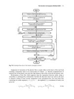
Root Cause Analysis for Quality Management

409

root

P(Y 1 )

P(Y 1 ∪ Y 2 )

P(Y 1 ∪ Y 3 )

P(Y 2 )

P(Y 1 ∪ Y n )

P(Y n−1 )

P(Y n )

P(Y n−1 ∪ Y n )

Fig. 1. Organization of the used multitree data structure

to find a node (sub-process) with a higher support in the branch below. This reduces
the time to find the optimal solution significantly, as a good portion of the tree to
traverse, can be omitted.
Algorithm 1 Branch & Bound algorithm for process optimization
¯
1: procedure T RAVERSE T REE(Y )
¯

Y := {sub-nodes of Y }
2:
3:
for all y ∈ Y do
4:
if N(X|y) > nmax and Q(X|y) ≥ qmin then
5:
nmax = N(X|y)
6:
end if
7:
if N(X|y) > nmax and Q(X|y) < qmin then
TraverseTree(y)
8:
9:
end if
10:
end for
11: end procedure

In many real world applications, the influence domain is mixed, consisting of
discrete data and numerical variables. To enable a joint evaluation of both influence
types, the numerical data is transformed into nominal data by mapping the continuous data onto pre-set quantiles. In most our applications, we chose 10%, 20%, 80%
and 90% quantile, as they performed the best.
Verification
The optimum of the problem (3) can only be defined in statistical terms, as in practice
the sample sets are small and the quality measures are only point estimators. Therefore, confidence intervals have to be used in order to get a more valid statement of
the real value of the considered PCI. In the special case, where the underlying data
follows a normal distribution, it is straight forward to construct a confidence interC
ˆ

val. As the distribution of Cp (C p denotes the estimator of Cp ) is known, a (1 − )%
ˆp
confidence interval for Cp is given by


410

Christian Manuel Strobel and Tomas Hrycej

⎡

ˆ
C(X) = ⎣Cp

2
n−1; 2

n−1

ˆ
, Cp

2
n−1;1− 2

n−1

⎤
⎦

(6)

For the other parametric basic indices, in general there exits no analytical solution
as they all have a non-centralized 2 distribution. Different numerical approximation
can be found in literature for Cpm ,Cpk and C pmk (see Balamurali and Kalyanasundaram (2002) and Bissel (1989)).
If there is no possibility to make an assumption about the distribution of the
data, computer based, statistical methods as the Bootstrap method are used to calculate a confidence intervals. In Balamurali and Kalyanasundaram (2002), the authors
present three different methods for calculating confidence intervals and a simulation
study. As result, the method called BCa-Method outperformed the other two methods, and therefore is used in our applications for assigning confidence intervals for
the non-parametric basic PCIs, as described in (3). For the Empirical Capability Index Eci a simulation study showed that the Bootstrap-Standard-Method, as defined in
Balamurali and Kalyanasundaram (2002), performed the best. A (1- )% confidence
interval for the Eci can be obtained by
ˆ
C(X) = Eci −

−1

(1 − )

ˆ
B , Eci +

−1

(1 − )

B

(7)

ˆ
where Eci denotes an estimator for Eci , B the Bootstrap standard deviation and −1
the inverse standard normal.
As the results of the introduced algorithm are based on sample sets, it is important to verify the soundness of the founded solutions. Therefore, the sample set
to analyze is to be randomly divided into two disjoint sets: training and test set. A
set of possible optimal sub-process is generated, by applying the describe algorithm
and the referenced Bootstrap-methods to calculate confidence intervals. In a second
step, the root cause analysis algorithm is applied to the test set. The final output is a
verified sub-process.

3 Computational results
A proof on concept was performed using data of a foundry plant and engine manufacturing in the premium automotive industry. The 32 analyzed sample sets comprised measurement results describing geometric characteristics like the position of
drill holes or surface texture of the produced products and the corresponding influence sets. The data sets consist of 4 to 14 different values, specifying for example a
particular machine number or a workers name. An additional data set, recording the
results of a cylinder twist measurement having 76 influence variables, was used to
evaluated the algorithm for numerical parameter sets. Each of the analyzed data sets
has at least 500 and at most 1000 measurement results.
The evaluation was performed for the non-parametric Cp and the empirical capability index Eci using the describe Branch and Bound principle. Additionally a


Root Cause Analysis for Quality Management

411

10000
Eci
Combinatorial
Cp

Time[s]

1000

100

10

1
1

16
Sample Set

31

Fig. 2. Computational time for combinatorial search vs. Branch and Bound

combinatorial search for the optimal solution was carried out to demonstrate the efficiency of our approach. The reduction of computational time, using the Branch and
Bound principle, amounted to two orders of magnitude in comparison to the combinatorial search as can be seen in Fig. 2. In average, the Branch and Bound method
outperformed the combinatorial search by the factor of 230. For the latter it took
in average 23 minutes to evaluating the available data sets. However, using Branch
and Bound reduced the computing time in average to only 5.7 seconds for the nonparametric Cp and to 7.2 seconds using the Eci . The search for an optimal solution
was performed to depth of 4, which means, that all sub-process have no more than
4 different influence variables. A higher depth level did not yield any other results,
as the support of the sub-processes diminishes with increasing number of influence
variables. Obviously, the computational time for finding the optimal sub-process increases with the number of influence variables and their values. This fact explains
the significant jump of the combinatorial computing time, as the first 12 sample sets
are made up of only 4 influence variables, whereas the others consist of up to 17
different influence variables.
As the number of influence parameters of the numerical data set where, compared

to the other data sets, significantly larger, it took, about 2 minutes to find the optimal
solution. The combinatorial search was not performed, as 76 influence variables each
with 4 values would have take too long.

4 Conclusion
In this paper we have presented a root cause analysis algorithm for process optimization, with the goal to identify those process parameters having a server impact on the


412

Christian Manuel Strobel and Tomas Hrycej

quality of a manufacturing process. The basic idea was to transform the search for
those quality drivers into a optimization problem and to identify optimal parameter
subsets using Branch and Bound techniques. This method allows for reducing the
computational time to identifying optimal solutions significantly, as the computational results show. Also a new class of convex process indices was introduced and a
particular specimen, the process capability index, Eci is defined. Since the search for
quality drivers in quality management is crucial to industrial practice, the presented
algorithm and the new class of indices may be useful for a broad scope of quality
and reliability problems.

References
BALAMURALI S. and KALYANASUNDARAM M. (2002): Bootstrap lower confidence limits for the process capability indices Cp, Cpk and Cpm. International Journal of Quality
& Reliability Management , 19, 1088–1097.
BISSELL A. (1990): How Reliable is Your Capability Index? Applied Statistics , 39, 331–340
.
KOTZ, S. and JOHNSON, N. (2002): Process Capability Indices – A Review, 1992 2000.
Journal of quality technology , 34, 2–53.
PEARN, W. and CHEN. K. (1997): Capability indices for non-normal distributions with an application in electrolytic capacitor manufacturing . Microelectronics Reliability, 37, 1853–
1858.

VÄNNMANN, K. (1995): A Unified Approach to Capability Indices. Statistica Sinica, 5,
805–820 .


The Application of Taxonomies in the Context of
Configurative Reference Modelling
Ralf Knackstedt and Armin Stein
European Research Center for Information Systems
{ralf.knackstedt, armin.stein}@ercis.uni-muenster.de
Abstract. The manual customisation of reference models to suite special purposes is an exhaustive task that has to be accomplished thoroughly to preserve, explicit and extend the inherit
intention. This can be facilitated by the usage of automatisms like those being provided by the
Configurative Reference Modelling approach. Thus, the reference model has to be enriched
by data describing for which scenario a certain element is relevant. By assigning this data to
application contexts, it builds a taxonomy. This paper aims to illustrate the advantage of the
usage of this taxonomy during three relevant phases of Configurative Reference Modelling,
Project Aim Definition, Construction and Configuration of the configurable reference model.

1 Introduction
Reference information models – in this context solely called reference models – give
recommendations for the structuring of information systems as best or common practices and can be used as a starting basis for the development of application specific
information system models. The better the reference models are matched with the
special features of individual application contexts, the bigger the benefit of reference
model use. Configurable reference models contain rules that describe how different
application specific variants are derived. Each of these rules is placed together with
a condition and an implication. Each condition describes one application context of
the reference model. The respective implication determines the relevant model variant. For describing the application contexts configuration parameters are used. Their
specification forms a taxonomy. Based upon a procedure model this paper highlights
the usefulness of taxonomies in the context of Configurative Reference Modelling.
Thus, the paper is structured as follows: First, the Configurative Reference Modelling
approach and its procedure model is being described. Afterwards, the usefulness of

the application of taxonomies is being shown during the respective phases. An outlook on future research areas concludes the paper.


374

Ralf Knackstedt and Armin Stein

2 Configurative Reference Modelling and the application of
taxonomies
2.1 Configurative Reference Modelling
Reference models are representations of knowledge recorded by domain experts to
be used as guidelines for every day business as well as for further research. Their
purpose is to structure and store knowledge and give recommendations like best or
common practices. They should be of general validity in terms of being applicable for
more than one user (see Schuette (1998); vom Brocke (2003); Fettke, Loos (2004)).
Currently 38 of them have been clustered and categorised, spanning domains like
logistics, supply chain management, production planing and control or retail (see
Braun, Esswein (2006)).
General applicability is a necessary requirement for a model to be characterised
as reference model, as it has to grant the possibility to be adopted by more than one
user or company. Thus, the reference model has to include information about different business models, different functional areas or different purposes for its usage.
A reference model for retail companies might have to cover economic levels like
Retail or Wholesale, trading levels like Inland trade or Foreign trade as well as functional areas like Sales, Production Planning and Control or Human Resource Management. While this constitutes the general applicability for a certain domain, one
special company usually needs just one suitable instance of this reference model, for
example Retail/Inland Trade, leaving the remaining information dispensable. This
yields the problem that the perceived demand of information for each individual will
be hardly met. The information delivered – in terms of models of different types
which might consist of different element types and hold different element instances
– might either be too little or too extensive, hence the addressee will be overburdened
on the one hand or insufficiently supplied with information on the other hand. Consequently, a person requiring the model for the purpose of developing the database

of a company might not want to be burdened with models of the technique Eventdriven Process Chain (EPC), whose purpose is to describe processes, but with Entity
Relationship Model (ERM), used to describe data structures. To compensate this in
a conventional manner, a complex manual customisation of the reference model is
necessary to meet the addressees demand. Another implication is the maintenance
of the reference model. Every time changes are committed to the reference model,
every instance has to be manually updated as well.
This is where Configurable Reference Models come into operation. The basic
idea is to attach parameters to elements of the integrated reference model in advance, defining the contexts to which these elements are relevant (see e. g. Knackstedt (2006)). In reference to the example given above this means that certain elements of the model might just be relevant for one of the economic levels – retail or
wholesale –, or for both of them. The user eventually selects the best suited parameters for his purpose and the respective configured model is generated automatically.
This leads to the conclusion that the lifecycle of a configurable reference model can
be divided into two parts called Development and Usage (see Schlagheck (2000)).


Taxonomies in the Context of Configurative Reference Modelling

375

The first part – relevant for the reference model developer – consists of the phases
Project Aim Definition, Model Technique Definition, Model Construction and Evaluation for the developer, whereas the second one – relevant for the user – includes the
phases Project Aim Definition, Search and Selection of existing and suitable reference models and Model Configuration. The configured model can be further adapted
to satisfy individual needs (see Becker et al. 2004). Several phases can be identified,
where the application of taxonomies can be of value, especially Project Aim Definition and Model Construction (for the developer) and Model Configuration (for the
user). Fig. 1 gives an overview of the phases, where the ones that will be discussed
in detail are solid, the ones actually not relevant are greyed out. The output of both
Development and Usage is printed in italics.

Fig. 1. Development and Usage of Configurable Reference Models

2.2 Project aim definition
During the first phase, Project Aim Definition, the developers have to agree on the

purpose of the reference model to build. They have to decide for which domain the
model should be used, which business models should be supported, which functional areas should be integrated to support the distribution for different perspectives
and so on. To structure these parameters, a morphological box has become apparent to be applicable. First, all instances for each possible characteristic have to be
listed. By shading the relevant parameters for the reference model, the developers
commit themselves to one common project aim and reduce the given complexity.
Thus, the emerging morphological box constitutes a taxonomy, implying the variants included in the integrated configurative reference model (see fig. 2; Mertens,
Lohmann (2000)). By generating this taxonomy, the developers get aware of all
possible included variants, thus getting a better overview of the to-be-state of the
model. One special variant of the model will later on be generated by choosing one
or a set of the parameters by the user. The choice of parameters should be supported by an underlying ontology that can be used throughout both Development
and Usage (see Knackstedt et al. (2006)). The developers have to decide whether
or not dependencies between parameters exist. In some cases, the choice of one


376

Ralf Knackstedt and Armin Stein

Fig. 2. Example of a morphological box, used as taxonomy. Becker et al. (2001)

specific parameter within one specific characteristic determines the necessity of another parameter within another characteristic. For example, the developers might
decide that the choice of ContactOrientation=MailOrder determines the choice
of PurchaseInitiationThrough=AND(Internet;Letter/Fax).
2.3 Construction
During the Model Construction phase, the configurable reference model has to be
developed in regards to the decisions made during the preceding phase Project Aim
Definition. The example in fig. 3 illustrates an EPC regarding the payment of a
bill, distinguishing whether the bill originates from a national or an international
source. If the origin of the bill is national, it can be paid immediately, otherwise it
has to be cross-checked by the international auditing. This scenario can only take

place, if both instances of the characteristic TradingLevel, namely InlandTrade
and ForeignTrade, are chosen. If all clients of a company are settled abroad or (in
the meaning of an exclusive or) all of them are inland, the check for the origin is
not necessary. The cross-check with the international auditing has only to take place,
if the bill comes from abroad. To store this information in the model, the respective parameters are attached to the respective model elements in form of a term and
can later be evaluated to true or false. Only if the equation is evaluated to true or
if there is no term attached to an element, the respective element may remain in the
configured model. Thus, for example, the function check for origin stays, if the term
TradingLevel=AND(Foreign;Inland) is true, which happens if both parameters
are selected. If only one is selected, the equation returns false and the element will
be removed from the model.


Taxonomies in the Context of Configurative Reference Modelling

377

Fig. 3. Annotated parameters to elements, resulting model variants

To specify these terms, which can get complex if many characteristics are used, a
term editor application has been developed, which enables the user to attach them
to the relevant elements. Here again, the ontology can support the developer by
automatically testing for correctness and reasonableness of dependent parameters
(see Knackstedt et al. (2006)). Opposite to dependencies, exclusions take into account that under certain circumstances parameters may not be chosen together. This
minimises the risk of defective modelling and raises the consistency level of the
configurable reference model. In the example given above, if the developer selects
SalesContactForm=VendingMachine, the parameter Beneficiary may not be
InvestmentGoodsTrade, as investment goods can hardly be bought via a vending machine. Thus, the occurrence of both statements concatenated with a logical
AND is not allowed. The same fact has to be regarded when evaluating dependencies:
If, like stated above, ContactOrientation=MailOrder determines the choice of

PurchaseInitiationThrough=AND(Internet;Letter/Fax), the same statement
may not occur with a preceded NOT. Again, the previously generated taxonomy can
support the developer by structurising the included variants.
2.4 Configuration
The Usage phase of a configurable reference model starts independently from its development. During the Project Aim Definition phase the potential user defines the pa-


378

Ralf Knackstedt and Armin Stein

rameters to determine which reference model best meets his needs. He has to search
for it during the Search and Selection phase. Once the user has selected a certain
configurable reference model, he uses its taxonomy to pick the parameters relevant
to his purpose. By automatically including dependent parameters, the ontology can
be of assistance in the same way as before, assuring that the mistakes made by the
user are reduced to a minimum (see Knackstedt et al. (2006)). For each parameter
– or set of parameters – a certain model variant is created. These variants have to
be differentiated by the aim of the configuration. On the one hand, the user might
want to configure a model that cannot be further adapted. This happens if a maximum of one parameter per characteristic is chosen. In this case, the ontology has to
consider dependencies as well as exclusions. On the other hand, if the user decides to
configure towards a model variant that should be configured again, exclusions may
not be considered. Both possibilities have to be covered by the ontology. Furthermore, a validation should cross-check against the ontology that no terms exist that
always equate to false. If an element is removed in every configuration scenario, it
should not have been integrated into the reference model in the first place. Thus, the
taxonomy can assist the user during the configuration phase by offering a set of parameters to choose from. Combined with an underlying ontology, the possibility of
making mistakes by using the taxonomy during the model adaptation is reduced to a
minimum.

3 Conclusion

As well as the ontology, the taxonomy used as a basic element throughout the phases
of Configurative Reference Modelling has to meet certain demands. Most importantly, the developers have to carefully select the constituting characteristics and associated parameters. It has to be possible for the user to distinguish between several
options, so they can make a clear decision to configure the model towards the variant
relevant for his purpose. This means that each parameter has to be understandable
and be delimited from the others, which – for example – can be arranged by supplying a manual or guide. Moreover, the parameters may neither be too abstract nor too
detailed. The taxonomy can be of use during the three relevant phases. As mentioned
before, the user has to be assisted in the usage of the taxonomy by automatically including or excluding parameters as defined by the ontology. Furthermore, only such
parameters should be chosen, that have an effect on the model that is comparative
to the necessary effort to identify it. Parameters that have no effect at all or are not
used should be removed as well, to decreases the complexity for both the developer
and the user. If the choice of a parameter results in the removal of only one element
and its identification takes a very long time, it should be removed from the taxonomy because of its little effect at high costs. Thus, the way the adaptation process is
supported by the taxonomy strongly depends on the associated ontology.


Taxonomies in the Context of Configurative Reference Modelling

379

4 Outlook
The resulting effect of the selection of one parameter to configure the model shows its
relevance and can be measured either by the quantity or by the importance of the elements that are being removed. Each parameter can be associated with a certain cost
that emerges due to the time it takes the user to identify it. Thus, cheap parameters are
easy to identify and have a huge effect once selected. Expensive parameters instead
are hard to identify and have little effect on the model. Further research should first
try to benchmark, which combinations of parameters of a certain reference model are
chosen most often. In doing so, the developer has the chance to concentrate on the
evolution of these parts of the reference model. Second, it should be possible to identify cheap parameters by either running simulations on reference models, measuring
the effect a parameter has – even in combination with other parameters –, or by auditing the behavior of reference model users – which is feasible in a limited way due
to the small distribution of configurable reference models. Third, configured models

should be rated with costs, so cheap variants can be identified and – the other way
round – the responsible parameters can be identified. To sum up, a objective function
should be developed, enabling the calculation of the costs for the configuration of a
certain model variant in advance by giving the selected parameters as input. It should
C(P )
have the form C(MV ) = n R(Pk ) with C(MV ) being the cost function of a certain
k=1
k
model variant derived from the reference model by using n parameters, C(Pk ) being
the cost function of a single parameter and R(Pk ) being a function weighting the relevance of a single parameter P, which is used for the configuration of the respective
model variant. Furthermore, the usefulness of the application of the taxonomy has to
be evaluated by empirical studies in every day business. This will be realised for the
configuration phase by integrating consultancies into our research and giving them a
taxonomy for a certain domain at hand. With the application of supporting software
tools, we hope that the adoption process of the reference model can be facilitated.

References
BECKER, J., DELFMANN, P. and KNACKSTEDT, R. (2004): Konstruktion von Referenzmodellierungssprachen – Ein Ordnungsrahmen zur Spezifikation von Adaptionsmechanismen fuer Informationsmodelle. Wirtschaftsinformatik, 46, 4, 251 – 264.
BECKER, J., UHR, W. and VERING, O. (2001): Retail Information Systems Based on SAP
Products. Springer Verlag, Berlin, Heidelberg, New York.
BRAUN, R. and ESSWEIN, W. (2006): Classification of Reference Models. In: Advances
in Data Analysis: Proceedings of the 30th Annual Conference of The Gesellschaft fuer
Klassifikation e.V., Freie Universitaet Berlin, March 8 – 10, 2006.
DELFMANN, P., JANIESCH, C., KNACKSTEDT, R., RIEKE, T. and SEIDEL, S. (2006):
Towards Tool Support for Configurative Reference Modelling – Experiences from a Meta
Modeling Teaching Case. In: Proceedings of the 2nd Workshop on Meta-Modelling and
Ontologies (WoMM 2006). Lecture Notes in Informatics. Karlsruhe, Germany, 61 – 83.
FETTKE, P. and LOOS, P. (2004): Referenzmodellierungsforschung. Wirtschaftsinformatik,
46, 5, 331 – 340.

380

Ralf Knackstedt and Armin Stein

KNACKSTEDT, R. (2006): Fachkonzeptionelle Referenzmodellierung einer Managementunterstuetzung mit quantiativen und qualitativen Daten. Methodische Konzepte zur Konstruktion und Anwendung. Logos-Verlag, Berlin.
KNACKSTEDT, R., SEIDEL, S. and JANIESCH, C. (2006): Konfigurative Referenzmodellierung zur Fachkonzeption von Data-Warehouse-Systemen mit dem H2-Toolset. In: J.
Schelp, R. Winter, U. Frank, B. Rieger, K. Turowski (Hrsg.): Integration, Informationslogistik und Architektur. DW2006, 21. – 22. Sept. 2006, Friedrichshafen. Lecture Notes
in Informatics. Bonn, Germany, 61 – 81.
MERTENS, P. and LOHMANN, M. (2000): Branche oder Betriebstyp als Klassifikationskriterien fuer die Standardsoftware der Zukunft? Erste Ueberlegungen, wie kuenftig betriebswirtschaftliche Standardsoftware entstehen koennte. In: F. Bodendorf, M. Grauer
(Hrsg.): Verbundtagung Wirtschaftsinformatik 2000. Shaker Verlag, Aachen, 110 – 135.
SCHLAGHECK, B. (2000): Objektorientierte Referenzmodelle fuer das Prozess- und Projektcontrolling. Grundlagen – Konstruktion – Anwendungsmoeglichkeiten. Deutscher
Universitaets-Verlag, Wiesbaden.
SCHUETTE, R. (1998): Grundsaetze ordnungsmaessiger Referenzmodellierung. Konstruktion konfigurations- und anpassungsorientierter Modelle. Deutscher UniversitaetsVerlag, Wiesbaden.
VOM BROCKE, J. (2003): Referenzmodellierung. Gestaltung und Verteilung von Konstruktionsprozessen. Logos Verlag, Berlin.


Two-Dimensional Centrality of a Social Network
Akinori Okada
Graduate School of Management and Information Sciences
Tama University, 4-1-1 Hijirigaoka Tama-shi, Tokyo 206-0022, Japan


Abstract. A procedure of deriving the centrality in a social network is presented. The procedure uses the characteristic values and the vectors of a matrix of friendship relationships
among actors. While the centrality of an actor has been usually derived by the characteristic
vector corresponding to the largest characteristic value, the present study uses not only the
characteristic vector corresponding to the largest characteristic value but also that corresponding to the second largest characteristic value. Each actor has two centralities. The interpretation
of two centralities, and the comparison with the additive clustering are presented.

1 Introduction

When we have a symmetric social network among a set of actors, where the relationship from actors j to k is equal to the relationship from actors k to j, the centrality
of each actor who constitutes a social network is very important to find the features
and the structure of the social network. The centrality of an actor represents the importance, significance, power, or popularity of the actor to form relationships with
the other actors in the social network. Several procedures to derive the centrality of
each actor in the social network have been introduced (ex. Hubbell (1965)). Bonacich
(1972) introduced a procedure to derive the centrality of an actor by using the characteristic (eigen) vector of a matrix of friendship relationships or friendship choices
among a set of actors. The matrix of friendship relationships which is dealt with by
these procedures is assumed to be symmetric.
The procedure of Bonacich (1972) is based on the characteristic vector corresponding to the largest characteristic (eigen) value. Each element of the characteristic
vector represents the centrality of each actor. The procedure has one good property
that the centrality of an actor is defined recursively by the weighted sum of the centralities of all actors, where the weight is the strength of the friendship relationship
between the actor and the other actors. The procedure was extended to deal with
an asymmetric matrix of friendship relationships (Bonachich (1991)), where (a) the
relationship from actors j to k is not same as that from actors k to j or (b) relationships between a set of actors and another set of actors. The first case (a) means


382

Akinori Okada

the one-mode two-way data, and the second case (b) means the two-mode two-way
data. These procedures utilized the characteristic vector which corresponds to the
largest characteristic value. Wright and Evitts (1961) also introduced a procedure to
derive the centrality of an actor utilizing the characteristic vectors which correspond
to more than one (largest) characteristic value. While Wright and Evitts (1961) say
the purpose is to derive the centrality, they focus their attention to summarize the relationships among actors just like applying factor analysis to the matrix of friendship
relationships.
The purpose of the present study is to introduce a procedure to derive the centrality of each actor of a social network by using the characteristic vectors which
correspond to more than one largest characteristic value of the matrix of friendship
relationships. Although the present procedure is based on more than one characteristic vectors, the purpose is to derive the centrality of actors but not to summarize

relationships among actors in a social network.

2 The procedure
The present procedure deals with a symmetric matrix of friendship relationships.
Suppose we are dealing with a social network consisits of n actors. Let A be an
n×n matrix representing friendship relationships among actors in a social network.
The ( j, k) element of A, a jk , represents the relationship between actor j and k; when
actors j and k are friends each other
a jk = 1,

(1)

and when actors j and k are not friends each other
a jk = 0.

(2)

Because the relationships among actors are symmetric, the matrix A is symmetric;
a jk = ak j .
The characteristic vectors of n×n matrix A which correspond to two largest characteristic values are derived. Each characteristic value represents the salience of the
centrality represented by the corresponding characteristic vector. The jth element of
a characteristic vector represents the centrality of actor j along the feature or the
aspect represented by the corresponding characteristic vector.

3 The analysis and the result
In the present study, the social network data among 16 families were analyzed
(Wasserman and Faust (1994, p. 744, Table B6)). The data show the marital relationships among 16 families. Thus the actor in the present data is the family. The
relationships are represented by a 16×16 matrix. Each element represents whether
there was a marital tie between two families corresponding to a row and a column

Two-Dimensional Centrality of a Social Network

383

(Wasserman and Faust (1994, p. 62)). The ( j, k) element of the matrix is equal to 1,
when there is a marital tie between families j and k, and is equal to 0, when there
is no marital tie between families j and k. In the present analysis, the unity was
embedded in the diagonal elements of the matrix of friendship relationships.
The five largest characteristic values of the 16×16 friendship relationship matrix
were 4.233, 3.418, 2.704, 2.007, and 1.930. The corresponding characteristic vectors
for the two largest characteristic values are shown in the second and the third columns
of Table 1.
Table 1. Characteristic vectors

Actor (Family)
1 Acciaiuoli
2 Albizzi
3 Barbadori
4 Bischeri
5 Castellani
6 Ginori
7 Guadagni
8 Lamberteschi
9 Medici
10 Pazzi
11 Peruzzi
12 Pucci
13 Ridolfi
14 Salviati

15 Strozzi
16 Tornabuoni

Dimension 1
Dimension 2
Characteristic values
4.233
3.418
0.129
0.210
0.179
0.328
0.296
0.094
0.283
0.086
0.383
0.039
0.339
0.000
0.301
0.137
0.404
0.281

0.134
0.300
0.053
-0.260
-0.353

0.123
0.166
0.076
0.434
0.117
-0.385
0.000
0.124
0.236
-0.382
0.285

Two characteristic values are 4.233 and 3.418 each of which represents the relative salience of the centrality over the all 16 actors along the feature or aspect shown
by each of the two characteristic vectors. The two centralities represent two different
features or aspects, called Dimensions 1 and 2 (see Figure 1), of the importance, significance, power, or popularity of actors. The second column, which represents the
characteristic vector corresponding the largest characteristic value, has non-negative
elements. These figures show the centrality of the 16 actors along the feature or the
aspects of Dimension 1. The larger value shows the larger centrality of an actor. Actor 15 has the largest value 0.404, and has the largest centrality among the 16 actors.
Actors 4, 9, 11, and 13 have larger centralities as well. Actor 12 has the smallest
value 0.000, and has the smallest centrality among the 16 actors. Actors 6, 8, and 10
also have small centralities.
The third column represents the characteristic vector corresponding to the second largest characteristic value. While the characteristic vector corresponding to the


384

Akinori Okada

largest characteristic value represented in the second column has all non-negative
elements, the characteristic vector corresponding to the second largest characteristic

value has negative elements. Actors 2 and 9 have larger positive elements. On the
contrary, actors 4, 5, 11, and 15 have substantive negative elements. The meaning
and the interpretation of the characteristic vector which corresponds to the second
largest characteristic value will be discussed in the next section.

4 Discussion
Two characteristic vectors each corresponding to the largest and the second largest
characteristic values represent the centralities of each actor along two different features or aspects of Dimensions 1 and 2. The 16 elements of the first characteristic vector seem to represent the overall (global) centrality or popularity of an actor
among the actors in the social network (cf. Scott (1991, pp. 85-89)). For each actor,
the number of ties with the other 15 actors were calculated. Each of the 16 figures
shows the overall centrality or popularity of the actor among actors in the social
network. The correlation coefficient between the elements of the first characteristic
vector and these figures were 0.90. This tells that the elements of the first characteristic vector shows the overall centrality or popularity of the actor in the social network.
This is the meaning of the feature or the aspect given by the first characteristic vector
of Dimension 1.
The jth element of the first characteristic vector shows the strength of actor j
in extending or accepting friendship relationships with the other actors in the social
network as a whole. The strength of the friendship relationship between actors j and
k along Dimension 1 is represented by the product of the jth and the kth elements of
the first characteristic vector. Because all elements of the first characteristic vector
are non-negative, the product of any two elements of the first characteristic vector is
non-negative. The larger the product is, the stronger the tie between two actors is.
The second characteristic vector has the positive (non-negative) and the negative
elements as well. Thus, there are three cases of the product of two elements of the
second characteristic vector;
(a) the product of two non-negative elements is non negative
(b) the product of two negative elements is positive, and
(c) the product of a positive element and a negative element is negative.
In the case of (a) the interpretation of the element of the second characteristic vector
is the same as that of the first characteristic vector. But in the cases of (b) and (c),

it is difficult to interpret the meaning of the elements by the same manner as that
for case (a). Because the element of the matrix of friendship relationships was defined by Equations (1) and (2), the larger value or the positive value of the product
of any two elements of the second characteristic vector shows the larger or positive
friendship relationship between two corresponding actors, and the smaller value or
the negative value shows the smaller or negative (friendship) relationship between
two corresponding actors. The product of two negative elements of the second characteristic vector is positive, and the positive figure shows the positive friendship rela-


Two-Dimensional Centrality of a Social Network

385

tionship between two actors. The product of the positive and the negative elements is
negative, and the negative figure shows the negative friendship relationship between
two actors.
The features or the aspect represented by the second characteristic vector can
be regarded as the local centrality or popularity within a subgroup (cf. Scott (1991,
pp.85-89)). As shown in Table 2, some actors have positive and some actors have
negative elements on Dimension 2 or the second characteristic vector. We can consider that there are two subgroups of actors; one subgroup consists of actors having
positive elements of the second characteristic vector, and another subgroup consists
of those having negative elements of the second characteristic vector, and that two
subgroups are not friendly. When two actors belong to the same subgroup, the product of the two corresponding elements of the second characteristic vector is positive
(cases (a) and (b) above), suggesting the positive friendship relationship between two
actors. On the other hand, when two actors belong to two different subgroups, which
means that one actor has the positive element and another actor has the negative element, the product of the two corresponding elements of the second characteristic
vector is negative (case (c) above), suggesting the negative friendship relationship
between two actors.
Table 1 shows that actor 4, 5, 11, and 15 have negative elements on the second
characteristic vector. This means that the second characteristic vector suggests two
subgroups of actors each consists of;

Subgroup 1: actors 1, 2, 3, 6, 7, 8, 9, 10, (12), 13, 14, and, 16
Subgroup 2: actors 4, 5, 11, and, 15
The two subgroups are graphically shown in Figure 1, where the horizontal dimension (Dimension 1) corresponds to the first characteristic vector, and vertical dimension (Dimension 2) corresponds to the second characteristic vector. Each actor is
represented as a point having the coordinate of the corresponding element of the first
characteristic vector on Dimension 1 and that of the second characteristic vector on
Dimension 2. Figure 1 shows that four members who belong to the second subgroup
are located closely each other and are separated from the other 12 actors. This seems
to validate the interpretation of the feature or the aspect represented by the second
characteristic vector.
The element of the second characteristic vector represents to which subgroup
each actor belongs by its sign (positive or negative). The element represents the centrality of an actor among actors within the subgroup to which the actor belongs,
because the product of the two elements corresponding to two actors belong to the
same subgroup is positive regardless of the sign of the elements. The absolute value
of the element of the second characteristic vector tells the local centrality or popularity among actors in the same subgroup to which the actor belongs, and the degree
of periphery or unpopularity among actors in another subgroup to which the actor
does not belong. The number of ties with actors who are in the same subgroup of
that actor is calculated for each actor. The correlation coefficient between the absolute value of the elements of the second characteristic vector and the number of ties
within a subgroup was 0.85. This tells that the absolute values of the elements of
the second characteristic vector shows the centrality of an actor in each of the two


386

Akinori Okada

subgroups. Because the correlation coefficient was derived over the two subgroups,
the centralities can be compared between subgroups 1 and 2.

Dimension 2

0.5
0.4
2 Albizzi

0.3

9 Medici

16 Tornabuoni
0.2 14 Salviati
7 Guadagni
10 Pazzi 6 Ginori
13 Ridolfi
0.1
1 Acciaiuoli
8 Lamberteschi
3 Barbadori
12 Pucci
-0.5 -0.4 -0.3 -0.2 -0.1 0
-0.1

0.1

0.2

-0.2

0.3 0.4 0.5
Dimension 1
4 Bischeri

-0.3

5 Castellani

-0.4

11 Peruzzi 15 Strozzi

-0.5
Fig. 1. Two-dimensional configuration of 16 families

The interpretation of the feature or the aspect of the second characteristic vector
reminds us of the ADCLUS model (Arabie and Carroll (1980); Arabie, Carroll, and
DeSarbo (1987); Shepard and Arabie, (1979)). In the ADCLUS model, each object
can belong to more than one cluster, and each cluster has its own weight which shows
the salience of that cluster. Table 2 shows the result of the application of ADCLUS
to the present friendship relationships data.
Table 2. Result of the ADCLUS analysis
Cluster
Cluster 1
Universal

Weight 1
1.88
-0.09

2

3

4

5

6

7

8

9 10 11 12 13 14 15 16

0 0
1 1

0
1

1
1

1
1

0
1

0
1

0
1

0
1

0
1

1
1

0
1

0
1

0
1

1
1

0
1

In Table 2, the second row represents whether each of the 16 actors belongs to
cluster 1 (when the element is 1) or does not belong to cluster 1 (when the element is

Two-Dimensional Centrality of a Social Network

387

0). The third row represents the universal cluster, to which all actors belong, representing the additive constant of the data (Arabie, Carroll, and DeSarbo (1987, p. 58)).
As shown in Table 2, actors 4, 5, 11, and 15 belong to cluster 1. These four actors are
coincide with those having the negative elements of the second characteristic vector
in Table 1.
The result derived by the analysis using ADCLUS and the result derived by using
the characteristic values and vectors are very similar. But they have several different
points. In the result derived by using ADCLUS, the strength of the friendship relationship between two actors is represented as the sum of two terms; (a) the weight
for the universal cluster, and (b) the weight for cluster 1 if the two actors belong to
cluster 1. The first term is constant for all combinations of any two actors, and the
second term is the weight for the first cluster (when two actors belong to cluster 1)
or zero (when one or none of the two actors belong to cluster 1). In using the characteristic vectors, the strength of the friendship relationship between two actors are
represented also as the sum of two terms; (a) the product of the two elements of the
first characteristic vector, and (b) the product of the two elements of the second characteristic vector. The first and the second terms are not constant for all combinations
of two actors but each combination of two actors has its own value, because each
actor has its own elements on the first and the second characteristic vectors. The first
and the second characteristic vectors are orthogonal, because the matrix of friendship relationships is assumed to be symmetric, and the two characteristic values are
different. The correlation coefficient between the first and the second characteristic
vectors is zero. The clusters derived by the analysis using ADCLUS does not have
the property even if two or more clusters were derived by the analysis.
In the present analysis only one cluster was derived by the analysis using ADCLUS. It seems interesting to compare the result derived by ADCLUS having more
than one cluster with the result based on the characteristic vectors corresponding
to the third largest and further characteristic values. The comparisons of the present
procedure with concepts used in the graph theory seem necessary to thoroughly evaluate the present procedure. The present procedure assumes that the strength of the
friendship relationship between actors j and k is represented by the product of the

centralities of actors j and k. But the strength of the friendship relationship between
two actors is defined as the sum of the centralities of the two actors by using the conjoint measurement (Okada (2003)). Which of the product or the sum of two centralities is more easily understood, or more practical in applications should be examined.
The original idea of the centrality has been extended to the asymmetric or rectangular social network (Bonacich (1991, 2001)). The present idea can also be extended
rather easily to deal with the asymmetric or the rectangular case as well.
Acknowledgments
The author would like to express his appreciation to Hiroshi Inoue for his helpful
suggestions to the present study. The author also wishes to thank two anonymous
referees for the valuable reviews which were very helpful to improve the earlier


388

Akinori Okada

version of the present paper. The present paper was prepared, in part, when the author
was at the Rikkyo (St. Paul’s) University.

References
ARABIE, P. and CARROLL, J.D. (1980): MAPCLUS: A Mathematical Programming Approach to Fitting the ADCLUS Model. Psychometrika, 45, 211–235.
ARABIE, P., CARROLL, J.D., and DeSARBO, W.S. (1987): Three-Way Scaling and Clustering. Sage Publications, Newbury Park.
BONACICH, P. (1972): Factoring and Weighting Approaches to Status Scores and Clique
Identification. Journal of Mathematical Sociology, 2, 113–120.
BONACICH, P. (1991): Simultaneous Group and Individual Centralities. Social Networks, 13,
155–168.
BONACICH, P. and LLOYD, P. (2001): Eigenvector-Like Measures of Centrality for Asymmetric Relations. Social Networks, 23, 191–201.
HUBBELL, C.H. (1965): An Input-Output Approach to Clique Identification. Socimetry, 28,
277–299.
OKADA, A. (2003): Using Additive Conjoint Measurement in Analysis of Social Network
Data. In: M. Schwaiger, and O. Opitz (Eds.): Exploratory Data Analysis in Empirical
Research. Springer, Berlin, 149-156.

SCOTT, J. (1991): Social Network Analysis: A Handbook. Sage Publications, London.
SHEPARD, R.N. and ARABIE, P. (1979): Additive Clustering: Representation of Similarities
as a Combinations of Discrete Overlapping Properties. Psychological Review, 86, 87–
123.
WASSERMAN, S. and FAUST, K. (1994): Social Network Analysis: Methods and Applications. Cambridge University Press, Cambridge.
WRIGHT, B. and EVITTS, M.S. (1961): Direct Factor Analysis in Sociometry. Sociometry,
24, 82–98.


Urban Data Mining Using Emergent SOM
Martin Behnisch1 and Alfred Ultsch2
1

2

Institute of industrial Building Production, University of Karlsruhe (TH),
Englerstraße 7, D-76128 Karlsruhe, Germany

Data Bionics Research Group
Philipps-University Marburg, D-35032 Marburg, Germany


Abstract. The term of Urban Data-Mining is defined to describe a methodological approach
that discovers logical or mathematical and partly complex descriptions of urban patterns and
regularities inside the data. The concept of data mining in connection with knowledge discovery techniques plays an important role for the empirical examination of high dimensional data
in the field of urban research. The procedures on the basis of knowledge discovery systems
are currently not exactly scrutinised for a meaningful integration into the regional and urban
planning and development process. In this study ESOM is used to examine communities in
Germany. The data deals with the question of dynamic processes (e.g. shrinking and growing
of cities). In the future it might be possible to establish an instrument that defines objective

criteria for the benchmark process about urban phenomena. The use of GIS supplements the
process of knowledge conversion and communication.

1 Introduction
Comparisons of cities and typological grouping processes are methodical instruments to develop statistical scales and criteria about urban phenomena. Harris started
in 1943, who ranked US cities according to industrial specialization data; many of
the other studies that followed added occupational data to the classification models.
Later on, in the 1970s, classification studies were geared to measuring social outcomes and shifted more towards the goals of public policy. Forst (1974) presents
an investigation of german cities by using social and economic variables. In Great
Britain, Craig (1985) employed a cluster analysis technique to classify 459 local
authority districts, based on the 1981 Census of Population. Hill et al. (1998) classified US cities by using the city’s population characteristics. Most of the mentioned
classification studies use economic, social, and demographic variables as a basis
for their classifications which are usually calculated by hierarchical algorithms (e.g.
WARD, K-Means). Geospatial objects are analysed by Demsar (2006). These former
approaches of city classification are summarized in Behnisch (2007).
The purpose of this article is to find groups (clusters) of communities with the
same dynamic characteristics in Germany (e.g. shrinking and growing of cities).


312

Martin Behnisch and Alfred Ultsch

The Application of Emergent Self Organizing Maps (ESOM) and the corresponding
U*C-Algorithm is proposed for the task of City Classification. The term of Urban
Data Mining (Behnisch, 2007) is defined to describe a methodological approach that
discovers logical or mathematical and partly complex descriptions of urban patterns
and regularities inside the data. The result can suggests a general typology and can
lead to the development of prediction models using subgroups instead of the total
population.

2 Inspection and transformation of data
Four variables were selected for the classification analysis. The variables characterise
a city’s dynamic behaviour. The data was created by the German BBR (Federal Office for Building and Regional Planning) and refers to the statistics of inhabitants
(V1 ), migration (V2 ), employment (V3 ) and mobility (V4 ). The dynamic processes are
characterised by positive or negative percentage quotations between the year 1999
and 2003. The inspection of data includes the visualisation in form of histograms,
QQ-Plots, PDE-Plots (Ultsch, 2003) and Box-Plots. The authors decided to use transformation measurements such as ladder of power to take into account restrictions of
statistics (Hand et al., 2001 or Ripley, 1996). Figure 1 and Figure 2 show an example
for the distribution of variables. As a result of pre-processing the authors find a mixture of two distributions with decision boundary zero in each of the four variables.
All variables are transformed by using Slog(x) = sign (x) · log(|x| + 1).

Fig. 1. QQ-Plot(inhabitants)

Fig. 2. PDE-Plot(Sloginhabitants)

The first hypothesis to the distribution of each variable is a bimodal distribution
of lognormal distributed data (Data > 0: skewed right, Data < 0: skewed left).
The result of the detailed examination is summarized in Table 1. The data follows
a lognormal distribution. Decision boundaries will be used to form a basis for a
manual classification process and support the interpretation of results.
Pertaining to the classification approach (e.g. U*-Matrix and subsequent U*CAlgorithm) and according to the Euclidian Distance the data need to be standardized.
Figure 3 shows Scatter-Plots of the transformed variables.


Urban Data Mining Using Emergent SOM

313

Table 1. Examination of the four distributions

Variable

Slog(Data)

inhabitants

bimodal distribution

migration

bimodal distribution

employment

bimodal distribution

mobility

multimodal distribution

Decision Boundaries
C1: Data ≤ 0
C2: Data > 0
C1: Data ≤ 0
C2: Data > 0
C1: Data ≤ 0
C2: Data > 0
C1: Data ≤ 0
C2: 0 < Data < 50
C3: Data ≥ 50

Size of Classes
[5820], 46,82%
[6610], 53,18%
[4974], 40,02%
[7456], 59,98%
[7492], 60,27%
[4938], 39,73%
[2551], 20,52%
[9317], 74,96%
[562], 4,52%

Fig. 3. Scatter-Plots of transformed variables

3 Method
In the field of urban planning and regional science data are usually multidimensional,
spatially correlated and especially heterogeneous. These properties make classical
data mining algorithms often inappropriate for this data, as their basic assumptions
cease to be valid. The power of self-organization allows the emergence of structure
in data and supports visualization, clustering and labelling concerning a combined
distance and density based approach. To visualize high-dimensional data, a projection from the high dimensional space onto two dimensions is needed. This projection
onto a grid of neurons is called SOM map. There are two different SOM usages. The
first are SOM, introduced by Kohonen (1982). Neurons are identified with clusters
in the data space (k-means SOM) and there are very few neurons. The second are


314

Martin Behnisch and Alfred Ultsch

SOM where the map space is regarded as a tool for the visualization of the otherwise
high dimensional data space. These SOM consist of thousands or tens of thousand
neurons. Such SOM allow the emergence of intrinsic structural features of the data
space and therefore they are called Emergent SOM (Ultsch, 1999). The map of an
ESOM preserves the neighbourhood relationships of the high dimensional data and
the weight vectors of the neurons are thought as sampling point of the data. The UMatrix has become the canonical tool for the display of the distance structures of
the input data on ESOM. The P-Matrix takes density information into account. The
combination of U-Matrix and P-Matrix leads to the U*Matrix. On this U*-Matrix a
cluster structure in the data set can be detected directly. Compare the examples in
Figure 4 using the same data to see in an appropriate way, whether there are cluster
structures.

Fig. 4. K-Means-SOM by Kaski et al. (1999), left and U*-Matrix, right

The often used finite grid as map has the disadvantage that neurons at the rim of
the map have very different mapping qualities compared to neurons in the centre vs.
the border. This is important during the learning phase and structures the projection.
In many applications important clusters appear in the corner of such a planar map.
Using ESOM methods for clustering has the advantage of a nonlinear disentanglement of complex structures.
The clustering of the ESOM can be performed at two different levels. The Bestmatch Visualization can be used to mark data points that represents a neuron with a
defined characteristic. Bestmatches and thus corresponding data points can be manually grouped into several clusters. Not all points need to be labelled, outliers are
usually easily detected and can be removed. Secondly the neurons can be clustered
by using a clustering algorithm, called U*C, which is based on grid projections and
uses distance and density information (Ultsch (2005)). In most times an aggregation
process of objects is necessary to build up a meaningful classification. Assigning a
name to a cluster is one of the most important processes in order to define the meaning of a cluster. The interpretation is based on the attribute values. Moreover it is
possible to integrate techniques of Knowledge Discovery to understand the structure
in a complementary form and support the finding of an appropriate cluster denomination. Examples are the symbolic algorithms such as SIG* or U-Know (Ultsch (2007))

Urban Data Mining Using Emergent SOM

315

which lead to significant properties for each cluster and a fundamental knowledge
based description.

4 Results
A first classification is based on the dichotomic characteristics of the four variables.
24 Classes are detected by using the decision boundaries (Variable > 0 or Variable
< 0). The further aggregation leads to the five classes of Table 2. The classed are content adressed to the approved pressure factors for urban dynamic development (population and employment). The purpose of such a wise classification was to sharpen
characteristics and to find a special label.
Table 2. Classes of Urban Dynamic Phenomena
Label
Shrinking of Inhabitants and Employment
Shrinking but influx
Growing of Employment
Growing of Inhabitants
Growing of Inhabitants and Employment

Inhabitants Migration Employment
low
low
low
low
high
low
low
high
high

low
high
high

An ESOM with 50x82 neurons is trained with the pre-processed data to proof
the defined structure. The corresponding U*-Map delivers a geographical landscape
of the input data on to a projected map (imaginary axis). The cluster boundaries are
expressed by mountains that means the value of height defines the distance between
different objects which is displayed on the z-Axis. A valley describes similar objects,
characterized by small U-heights on the U*-Matrix. Data points found in coherent
regions are assigned to one cluster. All local regions lying in the same cluster have
the same spatial properties.
The U*-Map (Island View) can be seen in Figure 5 in connection to the U*Matrix of Figure 6 including the clustering results of U*C-Algorithm with 11 classes.
The existing clusters are described by the U-Know Algorithm and the symbolic description is comparable to the dichotomic properties. The interpretation of the clustering results leads finally to the same five main classes realized by the content-based
aggregation. It is remarkable that the structure of the first classification can be recognized by using later Emergent SOM.
Figure 7 determines the five main cluster solution and displays the spatial structure of the classified objects. It is obvious to see that growing processes can be found
in the southern and western part of Germany and shrinking processes can be localized in the eastern part. Shrinking processes also exist in areas of traditional coal and
steel industry.