Data Analysis Machine Learning and Applications Episode 3 Part 3 pps

Analysis of Dwell Times in Web Usage Mining
Patrick Mair
1
and Marcus Hudec
2
1
Department of Statistics and Mathematics and ec3
Wirtschaftuniversität Wien
Augasse 2-6, 1090 Vienna, Austria

2
Department of Scientific Computing and ec3
University of Vienna
Universitätsstr. 5, 1010 Vienna, Austria

Abstract. In this contribution we focus on dwell times a user spends on various areas of a web
site within a session. We assume that dwell times may be adequately modeled by a Weibull
distribution which is a flexible and common approach in survival analysis. Furthermore we
introduce heterogeneity by various parameterizations of dwell time densities by means of
proportional hazards models. According to these assumptions the observed data stem from
a mixture of Weibull densities. Estimation is based on EM-algorithm and model selection
may be guided by BIC. Identification of mixture components corresponds to a segmentation
of users/sessions. A real life data set stemming from the analysis of a world wide operating
eCommerce application is provided. The corresponding computations are performed with the
mixPHM
package in R.
1 Introduction
Web Usage Mining focuses on the analysis of visiting behavior of users on a web
site. Common starting point are the so called click-stream data which are derived
from web-server logs and may be viewed as the electronic trace a user leaves on a
web site. Adequate modeling of the dynamics of browsing behavior is of particular

relevance for the optimization of eCommerce applications. Recently Montgomery
et al. (2004) proposed a dynamic multinomial probit model of navigation patterns
which lead to an remarkable increase of conversion rates. Park and Fader (2004) de-
veloped multivariate exponential-gamma models which enhance cross-site customer
acquisition. These papers indicate the potential that such approaches offer for web-
shop providers.
In this paper we will focus on modeling dwell times, i.e., the time a user spends
for viewing a particular page impression. They are defined by the time span between
two subsequent page requests and can be calculated by taking the difference between
the two logged time points when the page request have been issued. For the analysis
594 Patrick Mair and Marcus Hudec
of complex web sites which consist of a large number of pages it is often reasonable
to reduce the number of different pages by aggregating individual page-impressions
to semantically related page categories reflecting meaningful regions of the web site.
Analysis of dwell times is an important source of information with regard to
the relevance of the content for different users and the effectiveness of the page in
attracting visitors. In this paper we are particularly interested in segmentation of
users into various groups which exhibit a similar behavior with regard to the dwell
times they spend on various areas of the site. Such a segmentation analysis is an
important step towards a better understanding of the way a user interacts on a web
site. It is therefore of relevance with regard to the prediction of user behavior as well
as for a user-specific customization or even personalization of web sites.
2 Model specification and estimation
2.1 Weibull mixture model
Since survival analysis focuses on duration times until some event occurs (e.g. the
death of a patient in medical applications) it seems straightforward to apply these
concepts to the analysis of dwell times in web usage mining applications.
With regard to dwell time distributions we assume that they follow a Weibull
distribution with density function f (t)=OJt
J−1

exp(−Ot
J
), where O is a scale pa-
rameter and J the shape parameter. For modeling the heterogeneity of the observed
population, we assume K latent segments of sessions. While the Weibull assumption
holds within all segments, different segments exhibit different parameter values. This
leads to the underlying idea of a Weibull mixture model. For each page category p
(p = 1, ,P) under consideration the resulting mixture has the following form
f (t
p
)=
K

k=1
S
k
f (t
p
;O
pk
,J
pk
)=
K

k=1
S
k
O
pk

J
pk
t
J
pk
−1
p
exp(−O
pk
t
J
pk
p
) (1)
where t
p
represents the dwell time on page category p with mixing proportions S
k
which correspond to the relative size of each segment.
In order to reduce the number of parameters involved we impose restrictions
on the hazard rates of different components of the mixture respectively pages. An
elegant way of doing this is offered by the concept of Weibull proportional hazards
models (WPHM). The general formulation of a WPHM (see e.g., Kalbfleisch and
Prentice (1980)) is
h(t;Z)=OJt
J−1
exp(ZE). (2)
where Z is a matrix of covariates, and E are the regression parameters. The term
OJt
J−1

is the baseline hazard rate h
0
(t) due to the Weibull assumption and h(t;Z)
hazard proportional to h
0
(t) resulting from the regression part in the model.
Analysis of Dwell Times in Web Usage Mining 595
2.2 Parsimonious modeling strategies
We propose five different models with respect to different proportionality restrictions
in the hazard rates as to reduce the number of parameters. In the
mixPHM
package by
Mair and Hudec (2007) the most general model is called
separate
: The WPHM is
computed for each component and page separately. Hence, the hazard of session i
belonging to component k (k = 1, ,K) on page category p (p = 1, ,P)is
h(t
i,p
;1)=O
k,p
J
k,p
t
J
k,p
−1
i,p
exp(E1). (3)
The parameter matrices can be represented jointly as

/ =
⎛
⎜
⎝
O
1,1
O
1,P
.
.
.
.
.
.
.
.
.
O
K,1
O
K,P
⎞
⎟
⎠
(4)
for the scale parameters and
* =
⎛
⎜
⎝

J
1,1
J
1,P
.
.
.
.
.
.
.
.
.
J
K,1
J
K,P
⎞
⎟
⎠
(5)
for the shape parameters. Both the scale and the shape parameters can vary freely
and there is no assumption of hazard proportionality in the
separate
model. In fact,
the parameters (2 ×K ×P in total) are the same as they were estimated directly by
using a Weibull mixture model.
Next, we impose a proportionality assumption across the latent components. In
the classification version of the EM-algorithm (see next section) in each iteration step
we have a “crisp" assignment of each session to a component. Thus, if we consider

this component vector g as main effect in the WPHM, i.e., h(t;g), we impose pro-
portional hazards for the components across the pages (
main.g
in
mixPHM
). Again,
the elements of the matrix / of scale parameters can vary freely, whereas the shape
parameter matrix reduces to the vector * =(J
1,1
, ,J
1,P
). Thus, the shape param-
eters are constant over the components and the number of parameters is reduced to
K ×P + P.
If we impose page main effects in the WPHM, i.e., h(t; p) or
main.p
, respec-
tively, as before, the elements of / are not restricted at all but this time the shape
parameters are constant over the pages, i.e., * =(J
1,1
, ,J
1,K
). The total number of
parameters is now K ×P + K.
For the main-effects model h(t;g+ p) we impose proportionality restrictions on
both / and * such that the total number of parameters is reduced to K + P.For
the scale parameter matrix proportionality restrictions of this
main.gp
model hold
row-wise as well as column-wise:

/ =
⎛
⎜
⎝
O
1
c
2
O
1
c
P
O
1
.
.
.
.
.
.
.
.
.
.
.
.
O
K
c
2

O
K
c
P
O
K
⎞
⎟
⎠
=
⎛
⎜
⎜
⎜
⎝
O
1
O
P
d
2
O
1
d
2
O
P
.
.
.

.
.
.
.
.
.
d
K
O
1
d
K
O
1
⎞
⎟
⎟
⎟
⎠
. (6)
596 Patrick Mair and Marcus Hudec
The c- and d-scalars are proportionality constants over the pages and components, re-
spectively. The shape parameters are constant over the components and pages. Thus,
* reduces to one shape parameter J which implies that the hazard rates are propor-
tional over components and pages.
To relax the rather restrictive assumption with respect to / we can extend the
main effects model by the corresponding component-page interaction term, i.e.,
h(t;g ∗ p).In
mixPHM
notation this model is called

int.gp
. The elements of / can
vary freely whereas * is again reduced to one parameter only, leaving us with a total
number of parameters of K ×P + 1. With respect to the hazard rate this relaxation
implies again proportional hazards over components and pages.
2.3 EM-estimation of parameters
In order to estimate such mixtures of WPHM, we use the EM-Algorithm (Demp-
ster et al. (1977), McLachlan and Krishnan (1997)). In the E-Step we establish the
expected likelihood values for each session with respect to the K components. At
this point it is important to take into account the probability that a session i of com-
ponent k visits page p, denoted by Pr
k,p
, which is estimated by the corresponding
relative frequency. The elements of the resulting K ×P matrix are model parameters
and have to be taken into account when determining the total number of parameters.
The resulting likelihood W
k,p
(s
i
) for session i being in component k for each page p
individually, is
W
k,p
(s
i
)=

f (y
p
;

ˆ
O
k,p
,
ˆ
J
k,p
)Pr
k,p
(s
i
) if p was visited by s
i
1−Pr
k,p
(s
i
) if p was not visited by s
i
(7)
To establish the joint likelihood, a crucial assumption is made: independence
of the dwell times over page-categories. To make this assumption feasible, a well-
would be hierarchical, the independence assumption would not hold. Without this
independence assumption, a multivariate mixture Weibull model would have to be
fitted which takes into account the covariance structure of the observations. This
would require that each session must have a full observation vector of length p,i.e,
each page category is visited within each session which seems not to be realistic
within the context of dwell times in web usage mining.
However, for a reasonable independence assumption the likelihood over all pages
that session i belongs to component k is given by

L
k
(s
i
)=
P

p=1
W
k,p
(s
i
). (8)
Thus, by looking at each session i separately, a vector of likelihood values
<
i
=(L
1
(s
i
),L
2
(s
i
), ,L
k
(s
i
)) results.
At this point, the M-step is carried out. The

mixPHM
package provides three
different methods. The classical version of the EM-algorithm (maximization EM;
advised page categorization must be established. For instance, if some page-categories
Analysis of Dwell Times in Web Usage Mining 597
EMoption = "maximization"
in
mixPHM
) computes the posterior probabilities that
session i belongs to group k and does not make a group assignment within each
iteration step but rather updates the matrix of posterior probabilities Q. A faster EM-
version is proposed by Celeux and Govaert (1992) which they call classification EM
(
EMoption = "classification"
in
mixPHM
): Within each iteration step a group
assignment is performed due to sup
k
(<
i
). Hence, the computation of the posterior
matrix is not needed. A randomized version of the M-step considers a combination
of the approaches above: After the computation of the posterior matrix Q,aran-
domized group assignment is performed due to the corresponding probability values
(
EMoption = "randomization"
).
As usual, the joint likelihood L is updated at each EM-iteration l until a certain
convergence criterion H is reached, i.e.,




L
(l)
−L
(l−1)



< H. Theoretical issues about
the EM-convergence in Weibull mixture models can be found in Ishwaran (1996)
and Jewell (1982).
3 Real life example
In this section we use a real dataset of a large Austrian company which runs a web-
shop to demonstrate our modeling approach. We restrict empirical analysis to a sub-
set of 333 buying-sessions and 7 page-categories we perform a dwell time based clus-
tering with corresponding proportionality hazard assumptions by using the
mixPHM
package in R (R Development Core Team, 2007).
bestview checkout service figurines jewellery landing search
6 16 592 30 12 183 0 13
15 136 157 0 139 430 11 0
23 428 2681 17 2058 2593 56 186
37 184 710 52 12 450 34 0
61 0 874 307 570 6 25 53
The above extract of the data matrix shows the dwell times of 5 sessions, while we
coded non-visited page categories as 0’s.
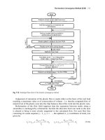
We start with a rather exploratory approach to determine an appropriate propor-
tionality model with an adequate number of clusters K.Byusingthe

msBIC
statement
we can accomplish such a heuristic model search.
> res.bic <- msBIC(x,K=2:5,method="all")
> res.bic
Bayes Information Criteria
Survival distribution: Weibull
K=2 K=3 K=4 K=5
separate 23339.27 23202.23 23040.01 22943.11
main.g 23355.66 23058.25 22971.86 22863.43
main.p 23503.73 23368.77 23165.60 23068.47
int.gp 23572.21 23422.51 23305.63 23075.76
main.gp 23642.74 23396.51 23271.72 23087.64
598 Patrick Mair and Marcus Hudec
It is obvious that the
main.g
model with K = 5 components fits quite well com-
pared to the other models (if we fit models for K > 5theBIC’s do not decrease
perspicuously anymore). For the sake of demonstration of the imposed hazard pro-
portionalities, we compare this model to the more flexible
separate
model. First, we
fit the two models again by using the
phmclust
statement which is the core routine
of the
mixPHM
package. The matrices of shape parameters *
sep
and *

g
, respectively,
for the first 5 pages (due to limited space) are:
> res.sep <- phmclust(x,5,method="separate")
> res.sep$shape[, 1:5]
bestview checkout service figurines jewellery
Component1 3.686052 2.692687 0.8553160 0.9057708 1.2503048
Component2 1.327496 3.393152 1.6260679 0.9716507 0.9941698
Component3 1.678135 2.829635 1.0417360 1.0706117 0.6902553
Component4 1.067241 1.847353 0.9860697 0.9339892 0.6321027
Component5 1.369876 2.030376 1.4565000 0.6434554 1.2414859
> res.g <- phmclust(x,5,method="main.g")
> res.g$shape[, 1:5]
bestview checkout service figurines jewellery
Component1 1.362342 2.981528 1.116042 0.7935599 0.9145463
Component2 1.362342 2.981528 1.116042 0.7935599 0.9145463
Component3 1.362342 2.981528 1.116042 0.7935599 0.9145463
Component4 1.362342 2.981528 1.116042 0.7935599 0.9145463
Component5 1.362342 2.981528 1.116042 0.7935599 0.9145463
The shape parameters in the latter model are constant across components. As a
consequence, page-wise within group hazard rates can vary freely for both models,
while the group-wise within page hazard rates can cross only for the
separate
model
(see Figure 1).
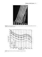
From Figure 2 it is obvious that the hazards are proportional across components
for each page. Note that due to space limitations, in both plots we only used three
selected pages to demonstrate the hazard characteristics. The hazard plots allow to
asses the relevance of different page categories with respect to cluster formation.
Similar plots for dwell time distributions are available.

4 Conclusion
In this work we presented a flexible framework to analyze dwell times on web pages
by adopting concepts from survival analysis to probability based clustering. Unob-
served heterogeneity is modeled by mixtures of Weibull distributed dwell times. Ap-
plication of the EM-algorithm leads to a segmentation of sessions.
Since the Weibull distribution is rather highly parameterized it offers a size-
able amount of flexibility for the hazard rates. A more parsimonious modeling may
either be achieved by posing proportionality restrictions on the hazards or mak-
ing use of simpler distributional assumptions (e.g., for constant hazard rates). The
Analysis of Dwell Times in Web Usage Mining 599
0 20406080100
0.00
0.01
0.02
0.03
0.04
0.05
bestview
Dwell Time
Hazard Function
Cluster 1
Cluster 2
Cluster 3
Cluster 4
Cluster 5
0 20406080100
0.00
0.01
0.02
0.03

0.04
0.05
service
Dwell Time
Hazard Function
Cluster 1
Cluster 2
Cluster 3
Cluster 4
Cluster 5
0 20406080100
0.00
0.01
0.02
0.03
0.04
0.05
figurines
Dwell Time
Hazard Function
Cluster 1
Cluster 2
Cluster 3
Cluster 4
Cluster 5
Fig. 1. Hazard Plot for Model
separate
mixPHM
package covers therefore additional survival distributions such as Exponen-
tial, Rayleigh, Gaussian, and Log-logistic.

A segmentation of sessions as it is achieved by our method may serve as a starting
point for optimization of a website. Identification of typical user behavior allows an
efficient dynamic modification of content as well as an optimization of adverts for
different groups of users.
0 20406080100
0.000 0.005
0.010 0.015
0.020 0.025
0.030
bestview
Dwell Time
Hazard Function
Cluster 1
Cluster 2
Cluster 3
Cluster 4
Cluster 5
0 20406080100
0.000 0.005
0.010 0.015
0.020 0.025
0.030
service
Dwell Time
Hazard Function
Cluster 1
Cluster 2
Cluster 3
Cluster 4
Cluster 5

0 20406080100
0.000 0.005
0.010 0.015
0.020 0.025
0.030
figurines
Dwell Time
Hazard Function
Cluster 1
Cluster 2
Cluster 3
Cluster 4
Cluster 5
Fig. 2. Hazard Plot for Model
main.g
600 Patrick Mair and Marcus Hudec
References
CELEUX, G., and GOVAERT, G. (1992). A Classification EM Algorithm for Clustering and
Two Stochastic Versions. Computational Statistics & Data Analysis, 14, 315–332.
DEMPSTER, A.P., LAIRD, N.M. and RUBIN, D.B. (1977). Maximum Likelihood from In-
complete Data via the EM-Algorithm. Journal of the Royal Statistical Society, Series B,
39, 1–38.
ISHWARAN, H. (1996). Identifiability and Rates of Estimation for Scale Parameters in Loca-
tion Mixture Models. The Annals of Statistics, 24, 1560-1571.
JEWELL, N.P. (1982). Mixtures of Exponential Distributions. The Annals of Statistics, 24,
479–484.
KALBFLEISCH, J.D. and PRENTICE, R.L. (1980): The Statistical Analysis of Failure Time
Data. Wiley, New York.
MAIR, P. and HUDEC, M. (2007). mixPHM: Mixtures of proportional hazard models.
R

package version 0.5.0:
/>MCLACHLAN, G.J. and KRISHNAN, T. (1997). The EM Algorithm and Extensions. Wiley,
New York.
MONTGOMERY, A.L., LI, S., SRINIVASAN, K. and LIECHTY, J.C. (2004). Modeling on-
line browsing and path analysis using clickstream data. Marketing Science, 23, 579–595.
PARK, Y. and FADER, P.S. (2004). Modeling browsing behavior at multiple websites. Mar-
keting Science, 23, 280–303
R Development Core Team. (2007). R: A Language and Environment for Statistical Comput-
ing. Vienna, Austria. (ISBN 3-900051-07-0)
Classifying Number Expressions in German Corpora
Irene Cramer
1
, Stefan Schacht
2
, Andreas Merkel
2
1
Dortmund University, Germany

2
Saarland University, Germany
{stefan.schacht, andreas.merkel}@lsv.uni-saarland.de
Abstract. Number and date expressions are essential information items in corpora and there-
fore play a major role in various text mining applications. However, so far number expressions
were investigated in a rather superficial manner. In this paper we introduce a comprehensive
number classification and present promising, initial results of a classification experiment using
various Machine Learning algorithms (amongst others AdaBoost and Maximum Entropy) to
extract and classify number expressions in a German newspaper corpus.
1 Introduction
In many natural language processing (NLP) applications such as Information Ex-

traction and Question Answering number expressions play a major role, e.g. ques-
tions about the altitude of a mountain, the final score of a football match, or the
opening hours of a museum make up a significant amount of the users’ informa-
tion need. However, common Named Entity task definitions do not consider num-
ber and date/time expressions in detail (or as in the Conference on Computational
Natural Language Learning (CoNLL) 2003 (Tjong Kim Sang (2003) do not incor-
porate them at all). We therefore present a novel, extended classification scheme for
number expressions, which covers all Message Understanding Conference (MUC)
(Chinchor (1998a)) types but additionally includes various structures not considered
in common Named Entity definitions. In our approach, numbers are classified ac-
cording to two aspects: their function in the sentence and their internal structure. We
argue that our classification covers most of the number expressions occurring in text
corpora. Based on this classification scheme we have annotated the German CoNLL
2003 data and trained various machine learning algorithms to automatically extract
and classify number expressions. We also plan to incorporate the number extraction
and classification system described in this paper into an open domain Web-based
Question Answering system for German. As mentioned above, the recognition of
certain date, time, and number expressions is especially important in the context of
Information Extraction and Question Answering. E. g. the MUC Named Entity def-
initions (Chinchor (1998b)) include the following basic types: date, time (
<TIMEX>
)
554 Irene Cramer, Stefan Schacht, Andreas Merkel
as well as monetary amount and percentage (
<NUMEX>
), and thus fostered the de-
velopment of extraction systems able to handle number and date/time expressions.
Famous Information Extraction systems developed in conjunction with MUC are
e.g. FASTUS (Appelt et al. (1993)) or LaSIE (Humphreys et al. (1998)). At that
time, many researchers used finite-state approaches to extract Named Entities. More

recent Named Entity definitions, such as CoNLL 2003 (Tjong Kim Sang (2003)),
aiming at the development of Machine Learning based systems, however, again ex-
cluded number and date expressions. Nevertheless, due to the increasing interest in
Question Answering and the TREC QA tracks (Voorhees et al. (2000)), recently, a
number of research groups investigate various techniques to fast and accurately ex-
tract information items of different types form text corpora and the Web, respectively.
Many answer typologies naturally include number and date expressions, e.g. the ISI
Question Answer Typology (Hovy et al. (2002)). Unfortunately, in the corresponding
papers only the whole Question Answering System’s performance is specified, we
therefore could not detect any performance values, which would be directly compa-
rable to our results. A very interesting and partially comparable (they only consider
a small fraction of our classification) work (Ahn et al. (2005)) investigates the ex-
traction and interpretation of time expressions. Their reported accuracy values range
between about 40% and 75%.
Paper Plan: This paper is structured as follows. Section 2 presents our classifica-
tion scheme and the annotation. Section 3 deals with the features and the experimen-
tal setting. Section 4 analyzes the results and comments on the future perspectives.
2 Classification of number expressions
Many researchers use regular expressions to find numbers in corpora, however, most
numbers are part of a larger construct such as ’2,000 miles’ or ’Paragraph 249 Bürg-
erliches Gesetzbuch’. Consequently, the number without its context has no meaning
or is highly ambiguous (2,000 miles vs. 2,000 cars). In applications such as Ques-
tion Answering it is therefore necessary to detect this additional information. Table 1
shows example questions that obviously ask for number expressions as answers. The
examples clearly indicate that we are not looking for mere digits but multi-word units
or even phrases consisting of a number and its specifying context. Thus, a number is
not a stand-alone information and, as the examples show, might not even look like
a number at all. This paper therefore proposes a novel, extended classification that
handles number expressions similar to Named Entities and thus provides a flexible
and scalable method to incorporate these various entity types into one generic frame-

work. We classify numbers according to their internal structure (which corresponds
to their text extension) and their function (which corresponds to their class).
We also included all MUC types to guarantee that our classification conforms
with previous work.
Classifying Number Expressions in German Corpora 555
Table 1. Example Questions and Corresponding Types
Q:
How far is the Earth from Mars?
miles? light-years?
Q:
How high is building X?
meters? floors?
Q:
What are the opening hours of museum X?
daily from 9 am to 5 pm
Q:
How did Dortmund score against Cottbus last weekend?
2:3
2.1 Classification scheme
Based on Web data and a small fraction of online available German newspaper cor-
pora (Frankfurter Rundschau
1
and die tageszeitung
2
) we deduced 5 basic types:
date
(including date and time expressions),
number
(covering count and measure expres-
sions),

itemization
(rank and score),
formula
,and
isPartofNE
(such as street
number or zipcode). As further analyses of the corpora showed most of the basic
types naturally split into sub-types, which also conforms to the requirements imposed
on the classification by our applications. The final classification thus comprises the
30 classes shown in table 2. The table additionally gives various examples and a short
explanation of the class’ sense and extension.
2.2 Corpora and annotation
According to our findings in Web data and newspaper corpora we developed guide-
lines which we used to annotate the German CoNLL 2003 data. To ensure a con-
sistent and accurate annotation of the corpus, we worked every part over in several
passes and performed a special reviewing process for critical cases. Table 3 shows
an exemplary extract of the data. It is structured as follows: the first column repre-
sents the token, the second column its corresponding lemma and the third column its
part-of-speech, the fourth column specifies the information produced by a chunker.
We did not change any of these columns. In column five, typically representing the
Named Entity tag, we added our own annotation. We replaced the given tag if we
found the tag
O
(
=other
) and appended our classification in all other cases.
3
While
annotating the corpora we met a number of challenges:
• Preprocessing: The CoNLL 2003 corpus exhibits a couple of erroneous sentence

and token boundaries. In fact, this is much more problematic for the extraction of
number expressions than for Named Entity Recognition, which is not surprising,
since it inherently occurs more frequently in the context of numbers.
• Very complex expressions: We found many
date.relative
and
date.regular
expressions, which are extremely complex types in terms of length, internal struc-
ture, as well as possible phrasing and therefore difficult to extract and classify. In
addition, we also observed very complex
number.amount
contexts and a couple
of broken sports score tables, which we found very difficult to annotate.
1
/>2
/>3
Our annotation is freely available for download. However, we cannot provide the original CoNLL 2003 data, which
you need to reconstruct our annotation.
556 Irene Cramer, Stefan Schacht, Andreas Merkel
Table 2. Overview of Number Classes
Name of Sub-Type Examples Explanation
date.period
for 3 hours, two decades time/date period, start
and end point not specified
date.regular
weekdays 10 am to 6 pm expressions like
opening hours etc.
date.time
at around 11 o’clock common time expressions
date.time.period

6-10 am duration, start and end
specified
date.time.relative
in two hours relative specification
tie: e.g. now
date.time.complete
17:40:34 time stamp
date.date
October 5 common date expressions
date.date.period
November 22-29, Wednesday duration,
to Friday, 1998/1990 start and end specified
date.date.relative
next month, in three days relative specification
tie: e.g. today
date.date.complete
July 21, 1991 complete date
date.date.day
on Monday all weekdays
date.date.month
last November all months
date.date.year
1993 year specification
number.amount
4 books, several thousand count, number of items
spectators
number.amount.age
aged twenty, Peter (27) age
number.amount.money
1 Mio Euros, 1,40 monetary amount

number.amount.complex
40 children per year complex counts
number.measure
18 degrees Celsius measurements not
covered otherwise
number.measure.area
30.000 acres specification of area
number.measure.speed
30 mph specification of speed
number.measure.length
100 km bee-line, 10 meters specification
of length, altitude,
number.measure.volume
43,7 l of rainfall, 230.000 specification of capacity
cubic meters of water
number.measure.weight
52 kg sterling silver, specification of weight
3600 barrel
number.measure.complex
67 l per square mile, complex measurement
30x90x45 cm
number.percent
32 %, 50 to 60 percent percentage
number.phone
069-848436 phone number
itemization.rank
third rank ranking e.g. in competition
itemization.score
9 points, 23:26 goals score e.g. in tournament
formula.variables


cos(x)
generic equations
formula.parameters
y = 4.132∗x
3
specific equations
• Ambiguities: In some cases we needed a very large context window to disam-
biguate the expressions they annotated. Additionally, we even found examples
which we could not disambiguate at all. E.g. über 3 Jahre with the possible trans-
lations more than 3 years or for 3 year. In German such structures are typically
disambiguated by prosody.
• Particular text type: A comparison between CoNLL and the corpora we used to
develop our guidelines showed that there might be a very particular style. We also
had the impression that the CoNLL training and test data differ with respect to
type distribution and style. We therefore based our experiments on the complete
data and performed cross-validation.
Classifying Number Expressions in German Corpora 557
We think that the thus annotated corpora represent a valuable resource, especially,
given the well-known data sparseness for German.
Table 3. Extract of the Annotated CoNLL 2003 Data
Am am APPRART I-PC date.date.complete
14. 14. ADJA I-NC date.date.complete
August August NN I-NC date.date.complete
1922 @card@ CARD I-NC date.date.complete
rief rufen VVFIN I-VC O
er er PPER I-NC O
den d ART B-NC O
katholischen katholisch ADJA I-NC O
Gesellenverein Gesellenverein NN I-NC O

ins ins APPRART I-PC O
Leben Leben NN I-NC O
$.O O
Furthermore, our findings during the annotation process again emphasized the
need of an integrated concept of number expressions and Named Entities: we found
467
isPartofNE
items, which are extremely difficult to classify without any hint
about proper names in the context window.
3 Experimental evaluation
3.1 Features
Our features (see table 4 for details) are adapted from those reported in previous work
on Named Entity Recognition (e.g. Bikel et al. (1997), Carreras et al. (2003)). We
based the extraction on a very simple and fast analysis of the tokens combined with
shallow grammatical clues. To additionally capture information about the context we
used a sliding window of five tokens (the word itself, the previous two, the following
two).
3.2 Classifiers
To get a feeling for the expectable performance, we conducted a preliminary test
by experimenting with Weka (Witten et al. (2005)). For this purpose we ran the
Weka implementations of a Decision Tree, k-Nearest Neighbor, and Naive Bayes
algorithm with the standard settings and no preprocessing or tuning. Because of pre-
vious, promising experiences with AdaBoost (Carreras et al. (2003)) and Maximum
Entropy in similar tasks, we decided to also apply these two classifiers. We used the
maxent
implementation of the Maximum Entropy algorithm
4
. For the experiments
with AdaBoost we used our own
C++

implementation, which we tuned for large
sparse feature vectors with binary entries.
4
/>558 Irene Cramer, Stefan Schacht, Andreas Merkel
Table 4. Overview of Features Used
feature group features
only digit strings 2-digit integer [30-99], other 2-digit integer, 4-digit
integer [1000-2100], other 4-digit integer, other integer
digit and non-digit strings 1-digit or 2-digit followed by point, 4-digit with central point
or colon, any digit sequence with point, colon, comma,
comma and point, hyphen, slash, or other non-digit character
non-digit strings any character sequence max length 3, any character sequence,
followed by point, any character sequence with slash,
any character sequence
grammar part-of-speech tag, lemma
window all features mentioned above for window +/-2
3.3 Results
The performance of the Decision Tree, k-Nearest Neighbor, Naive Bayes, and Maxi-
mum Entropy algorithm is on average mediocre, as Table 5 reveals. On the contrary,
our AdaBoost implementation shows satisfactory or even good f-measure values for
almost all cases and thus significantly outperforms the rest of the classifiers.
Table 5. Overview of the F-Measure Values (AB: AdaBoost, DT: Decision Tree, KNN: k-
Nearest Neighbor, ME: Maximum Entropy, NB: Naive Bayes)
class AB DT KNN ME NB class AB DT KNN ME NB
other 0.99 0.99 0.98 0.99 0.97 itemization.score 0.83 0.43 0.40 0.78 0.04
date 0.37 0.13 0.21 0.24 0.19 number 0.64 0.00 0.08 0.00 0.00
date.date 0.67 0.73 0.67 0.74 0.09 number.amount 0.33 0.53 0.25 0.67 0.26
date.date.complete 0.72 0.61 0.74 0,49 0.20 number.amount.age 0.62 0.28 0.14 0.45 0.02
date.date.day 0.53 0.15 0.14 0.20 0.06 number.amount.complex 0.09 0.00 0.00 0.00 0.00
date.date.month 0.37 0.05 0.08 0.24 0.00 number.amount.money 0.82 0.45 0.28 0.79 0.30

date.date.period 0.43 0.38 0.36 0.45 0.09 number.measure 0.22 0.16 0.00 0.17 0.00
date.date.relative 0.54 0.36 0.16 0.59 0.00 number.measure.area 0.88 0.10 0.00 0.40 0.00
date.date.year 0.82 0.73 0.58 0.76 0.60 number.measure.complex 0.34 0.21 0.19 0.22 0.09
date.regular 0.49 0.43 0.37 0.54 0.14 number.measure.length 0.69 0.17 0.11 0.39 0.01
date.time 0.87 0.76 0.67 0.83 0.45 number.measure.speed 0.91 0.17 0.18 0.00 0.00
date.time.period 0.41 0.40 0.46 0.38 0.31 number.measure.volume 0.66 0.06 0.00 0.00 0.00
date.time.relative 0.38 0.02 0.07 0.00 0.00 number.measure.weight 0.49 0.00 0.00 0.00 0.00
itemization 0.21 0.28 0.23 0.17 0.12 number.percent 0.83 0.32 0.10 0.56 0.06
itemization.rank 0.84 0.31 0.23 0.70 0.00 number.phone 0.96 0.85 0.89 0.95 0.65
Table 5 also shows that there are classes with a consistently poor performance,
such as
number.amount.complex
,
number. measure
,or
itemization
, and a con-
sistently good performance, such as
number.phone
or
date.date.year
. We think
that this correlates with the amount of data as well as the heterogeneity of the classes.
For instance,
number.measure
and
itemization
items occur indeed frequently in
the corpus but these two classes are–according to our definition–’garbage collec-
tors’ and therefore much less homogenous. In contrast, there are classes, such as

date.time.period
or
date.regular
, with rather low f-measure values but a very
precise definition; we admittedly suspect that the annotation of these types in our
corpora might be inconsistent or inaccurate. We also suppose that there are number
Classifying Number Expressions in German Corpora 559
expressions which exhibit an exceedingly large variety of phrasing. As a matter of
fact, these are inherently difficult to learn if the data do not feature sufficient cover-
age.
Table 6. Overview of the Precision Values (AB: AdaBoost)
class AB class AB class AB
other 0.98 date.time 0.88 number.amount.complex 0.39
date 0.61 date.time.period 0.54 number.percent 0.87
date.date 0.75 date.time.relative 0.50 number.phone 0.96
date.date.complete 0.79 itemization 0.34 number.measure 0.70
date.date.day 0.83 itemization.rank 0.88 number.measure.area 0.93
date.date.month 0.79 itemization.score 0.91 number.measure.length 0.85
date.date.year 0.85 number 0.81 number.measure.speed 0.94
date.date.relative 0.73 number.amount 0.48 number.measure.volume 0.76
date.date.period 0.65 number.amount.age 0.79 number.measure.weight 0.56
date.regular 0.68 number.amount.money 0.89 number.measure.complex 0.65
Fortunately, there are is a number of classes with a pretty high f-measure value–
that is more than 0.8–for at least one of the five classifiers, e.g.
date.date.year
,
itemization.rank
, and
number.phone
. More importantly there are, as Table 6

shows, only six classes with a precision value of less than 0.6. We are therefore very
confident to be able to successfully integrate the AdaBoost implementation of our
number extraction component into a Web-based open domain Question Answering
System, since in a Web-based framework the focus tends to be on precision rather
than coverage or recall.
4 Conclusions and future work
We presented a novel, extended number classification and developed guidelines to
annotate a German newspaper corpus accordingly. On the basis of our annotated data
we have trained and tested five classification algorithms to automatically extract and
classify them with promising evaluation results. However, the accuracy is still low
for some classes, especially for the small or heterogenous ones. But we feel confident
to improve our system by incorporating selected training data, especially, in the case
of small classes. To find the weak points in our system, we plan to perform a detailed
analysis of all number types and their precision, recall, and f-measure values. We
also consider a revision of our annotation, because there still might be inconsistently
and inaccurately annotated sections in the corpus. As mentioned above, the CoNLL
2003 data exhibit a typical newspaper style, which might limit the applicability of
our system to particular corpus types (although, initial experiments with Web data
do not support this skepticism). We therefore intend to augment our training data
with Web texts annotated according to our guidelines. In addition, we plan to ex-
periment with an expanded feature set and several pre-processing methods such as
feature selection and normalization. Research in the area of Named Entity extraction
shows that multiple classifier systems or the concept of multi-view learning might be
560 Irene Cramer, Stefan Schacht, Andreas Merkel
especially effective in our application. We therefore plan to investigate several clas-
sifier combinations and also take a hybrid approach–combining grammar rules and
statistical methods–into account. We plan to integrate our number extraction system
into a Web-based open domain Question Answering system for German and hope to
improve the coverage and performance of the answer types processed. While there
is still room for improvement, we think–considering the complexity of our task–the

achieved performance is surprisingly good.
References
AHN, D., FISSAHA ADAFRE, S. and DE RIJKE, M. (2005): Recognizing and Interpreting
Temporal Expressions in Open Domain Texts. S. Artemov et al. (eds): We Will Show
Them: Essays in Honour of Dov Gabbay, Vol 1., College Publications.
APPELT, D., BEAR, J., HOBBS, J., ISRAEL, D., KAMEYAMA, M., STICKEL, M. and
TYSON, M. (1993): FASTUS: A Cascaded Finite-State Tranducer for Extracting Infor-
mation from Natural-Language Text. SRI International.
BIKEL, D., MILLER, S., SCHWARTZ, R. and WEISCHEDEL, R. (1997): Nymble: a high-
performance learning name-finder. Proceedings of 5th ANLP.
CARRERAS, X., MÀRQUEZ, L. and PADRÓ, L. (2003): A Simple Named Entity Extractor
using AdaBoost. Proceedings of CoNLL-2003
CHINCHOR, N. A. (1998a): Overview of MUC-7/MET-2. Proceedings of the Message Un-
derstanding Conference 7.
CHINCHOR, N. A. (1998b): MUC-7 Named Entity Task Definition (version 3.5) Proceedings
of the Message Understanding Conference 7.
HOVY, E. H., HERMJAKOB, U. and RAVICHANDRAN, D. (2002): A Question/Answer Ty-
pology with Surface Text Patterns. Proceedings of the DARPA Human Language Tech-
nology conference (HLT).
HUMPHREYS, K., GAIZAUSKAS, R., AZZAM, S., HUYCK, C., MITCHELL, B. CUN-
NINGHAM, H. and WILKS, Y. (1998): University of Sheffield: Description of the
LaSIE-II System as Used for MUC-7. Proceedings of the 7th Message Understanding
Conference (MUC-7).
TJONG KIM SANG, E. F. and DE MEULDER, F. (2003): Introduction to the CoNLL Shared
Task: Language-Independent Named Entity Recognition. Proceedings of the Conference
on Computational Natural Language Learning.
VOORHEES, E. and TICE, D. (2000): Building a Question Answering Test Collection. Pro-
ceedings of SIGIR-2000.
WITTEN, I. H. and FRANK, E. (2005): Data Mining: Practical machine learning tools and
techniques. 2nd Edition, Morgan Kaufmann, San Francisco.

Comparing the University of South Florida
Homograph Norms with Empirical Corpus Data
Reinhard Rapp
Universitat Rovira i Virgili, GRLMC, Tarragona, Spain

Abstract. The basis for most classification algorithms dealing with word sense induction and
word sense disambiguation is the assumption that certain context words are typical of a par-
ticular sense of an ambiguous word. However, as such algorithms have been only moderately
successful in the past, the question that we raise here is if this assumption really holds. Start-
ing with an inventory of predefined senses and sense descriptors taken from the University
of South Florida Homograph Norms, we present a quantitative study of the distribution of
these descriptors in a large corpus. Hereby, our focus is on the comparison of co-occurrence
frequencies between descriptors belonging to the same versus to different senses, and to the
effects of considering groups of descriptors rather than single descriptors. Our findings are that
descriptors belonging to the same sense co-occur significantly more often than descriptors be-
longing to different senses, and that considering groups of descriptors effectively reduces the
otherwise serious problem of data sparseness.
1 Introduction
Resolving semantic ambiguities of words is among the core problems in natural lan-
guage processing. Many applications, such as text understanding, question answer-
ing, machine translation, and speech recognition suffer from the fact that – despite
numerous attempts (e.g. Kilgarriff and Palmer, 2000; Pantel and Lin, 2002; Rapp,
2004) – there is still no satisfactory solution to this problem. Although it seems rea-
sonable that the statistical approach is the method of choice, it is not obvious what
statistical clues should be looked at, and how to deal with the omnipresent problem
of data sparseness.
In this situation, rather than developing another algorithm and adding it to the
many that already exist, we found it more appropriate to systematically look at the
empirical foundations of statistical word sense induction and disambiguation (Rapp,
2006). The basic assumption underlying most if not all corpus-based algorithms is

the observation that each sense of an ambiguous word seems to be associated with
certain context words. These context words can be considered to be indicators of this
particular sense. For example, context words such as grow and soil are typical of the
flora meaning of plant, whereas power and manufacture are typical of its industrial
612 Reinhard Rapp
meaning. Being associated implies that the indicators should co-occur significantly
more often than expected by chance in the local contexts of the respective ambiguous
word. Looking only at local contexts can be justified by the observation that for
humans in almost all cases the local context suffices to achieve an almost perfect
disambiguation performance, which implies that the local context carries all essential
information.
If there exist several indicators of the same sense, then it can not be ruled out,
but it is probably unlikely that they are mutually exclusive. As a consequence, in
the local contexts of an ambiguous word indicators of the same sense should have
co-occurrence frequencies that are significantly higher than chance, whereas for in-
dicators relating to different senses this should not be the case or, if so, only to a
lesser extend.
Our aim in this study is to quantify this effect by generating statistics on the co-
occurrence frequencies of sense indicators in a large corpus. Hereby, our inventory
of ambiguous words, their senses, and their sense indicators is taken from the Uni-
versity of South Florida Homograph Norms (USFHN), and the co-occurrence counts
are taken from the British National Corpus (BNC). As previous work (Rapp, 2006)
showed that the problem of data sparseness is severe, we also propose a methodology
for effectively dealing with it.
2 Resources
For the purpose of our study a list of ambiguous words is required together with
their senses and some typical indicators of each sense. As described in Rapp (2006),
such data was extracted from the USFHN. These norms were compiled by collecting
the associative responses given by test persons to a list of 320 homographs, and
by manually assigning each response to one of the homograph’s meanings. Further

details are given in Nelson et al. (1980).
For the current study, from this data we extracted a list of all 134 homographs
where each comes together with five associated words that are typical of its first
sense, and another five words that are typical of its second sense. The first ten en-
tries in this list are shown in Table 1. Note that for reasons to be discussed later we
abandoned all homographs where either the first or the second sense did not receive
at least five different responses. This was the case for 186 homographs, which is the
reason that our list comprises only 134 of the 320 items. As in the norms the ho-
mographs were written in uppercase letters only, we converted them to that spelling
of uppercase and lowercase letters that was found to have the highest occurrence
frequency in the BNC. In the few cases where subjects had responded with multi
word units, these were disregarded unless one of the words carried almost all of the
meaning.
Another resource that we use is the BNC, which is a balanced sample of written
and spoken English that comprises about 100 million words. As described in Rapp
(2006), this corpus was used without special pre-processing, and for each of the
Comparing Homograph Norms with Corpus Data 613
134 homographs concordances were extracted comprising text windows of particular
widths (e.g. ±10 words around the given word).
Table 1. Some homographs and the top five associations for their two main senses.
HOMOG. SENSE 1 SENSE 2
bar drink beer tavern stool booze crow bell handle gold press
beam wood ceiling house wooden building light laser sun joy radiate
bill pay money payment paid me John Uncle guy name person
block stop tackle road buster shot wood ice head cement substance
bluff fool fake lie call game cliff mountain lovely high ocean
board wood plank wooden ship nails chalk black bill game blackboard
bolt nut door lock screw close jump run leap upright colt
bound tied tie gagged rope chained jump leap bounce up over
bowl cereal dish soup salad spoon ball pins game dollars sport

break ruin broken fix tear repair out even away jail fast
3 Approach
For each homograph we were interested in three types of information. One is the av-
erage intra-sense association strength for sense 1, i.e. the average association strength
between all possible pairs of words belonging to sense 1. Another is the average intra-
sense association strength for sense 2, which is calculated analogously. And a third is
the average inter-sense association strength between senses 1 and 2, i.e. the average
association strength between all possible pairs of words under the condition that the
two words in each pair must belong to different senses. Using the homograph bar,
Figure 1 illustrates this by making explicit all pairs of associations that are involved
in the computation of the average strengths. Hereby the association strength a
ij
be-
tween two words i and j is computed as the number of lines in the concordance where
both words co-occur ( f
ij
) divided by the product of the concordance frequencies f
i
and f
j
of the two words:
a
ij
=
f
ij
f
i
· f
j

This formula normalizes for word frequencies and thereby avoids undesired ef-
fects resulting from their tremendous variation. In cases where the denominator was
zero we assigned a score of zero to the whole expression. Note that the counts in the
denominator are observed word frequencies within the concordance, not within the
entire corpus.
Whereas the above formula computes association strengths for single word pairs,
what we are actually interested in are the three types of average association strengths
a
ij
as depicted in Figure 1. For ease of reference, in the remainder of the paper we
use the following notation:
614 Reinhard Rapp
Fig. 1. Computation of average intra-sense and inter-sense association strengths exemplified
using the associations to the homograph bar.
S1 = average a
ij
over the 10 word pairs relating to sense 1
S2 = average a
ij
over the 10 word pairs relating to sense 2
SS = average a
ij
over the 25 word pairs relating to senses 1 and 2
The reasoning behind computing average scores is to minimize the problem of
data sparseness by taking many observations into account. An important feature of
our setting is that if we – as described in the next section – increase the number
of words that we consider (5 per sense in the example of Figure 1), the number of
possible pairs increases quadratically, which means that this should be an effective
measure for solving the sparse-data problem. Note that we could not sensibly go be-
yond five words in this study, as the number of associations provided in the USFHN

is rather limited for each sense, so that there is only a small number of homographs
where more than five associations are provided for the two main senses.
When comparing the scores S 1, S2, and SS, what should be our expectations?
Most importantly, as discussed in the introduction, same-sense co-occurrences should
be more frequent than different-sense co-occurrences, thus both S1andS2 should be
larger than SS. But should S1andS2 be at the same level or not? To answer this
question, recall that S1 relates to the main sense of the respective homograph, and
S2 to its secondary sense. If both senses are similarly frequent, then both scores are
based on equally good data and can be expected to be at similar levels. However, if
the vast majority of cases relates to the main sense, and if the secondary sense occurs
only a few times in the corpus (an example being the word can with its frequent verb
and infrequent noun sense), then the co-occurrence counts – which are always based
on the entire concordance – would mainly reflect the behavior of the main sense, and
might be only marginally influenced by the secondary sense. As will be shown in
the next section, for our data S2 turns out to be at about the same level as S1. Note,
however, that this could be an artefact of our choice of homographs, as we had to
Comparing Homograph Norms with Corpus Data 615
pick those where the subjects provided at least five different associative responses to
each sense.
4 Results and discussion
Following the procedure as described in the previous section, Table 2 shows the first
10 out of 134 results for the homograph-based concordances of width ±100 with
five associations being considered for each sense (for a list of these associations see
Table 1). In all but two cases the values for S1 and S2 are – as expected – both larger
than those for SS. Only the homographs bill and break behave unexpectedly. In the
first case this may be explained by our way of dealing with capitalization (see section
2), in the second it is probably due to continuation associations such as break – out
and break – away, which are not specifically dealt with in our system.
Note that the above qualitative considerations are only meant to give an impres-
sion of some underlying sophistications which make it unrealistic to expect an overall

accuracy of 100%. Nevertheless, exact quantitative results are given in Table 3. For
several concordance widths, this table shows the number of homographs where the
results turn out to be as expected, i.e. S1 > SS and S2 > SS (columns 3 and 4). Perfect
results would be indicated by values of 134 (i.e. the total number of homographs) in
each of these two columns. The table also shows the number of cases where S1 > S2,
and – as an additional information – the number of cases where S1andS2, S2and
SS, and S1andS2 are equal. As S1, S2, and SS are averages over several floating
point values, their equality is very unlikely except for the case when all underlying
co-occurrence scores are zero, which is only true if data is very sparse. Thus the
equality scores can be seen as a measure of data sparseness. As data sparseness af-
fects all three equality scores likewise, they can be expected to be at similar levels.
Nevertheless, to confirm this expectation empirically, scores are shown for all three.
Table 2. Results for the first ten homographs (numbers to be multiplied by 10
−6
).
Homograph S1 S2 SS
Homograph S1 S2 SS
bar 223 199 37 board 205 799 53
beam 1305 1424 123
bolt 1794 3747 962
bill 166 95 202
bound 675 692 139
block 194 945 112
bowl 327 644 25
bluff 934 2778 226
break 156 63 95
In Table 3, for each concordance width we also distinguish four cases where
each relates to a different number of associations (or sense indicators) considered.
Whereas so far we always assumed that for each homograph we take five associa-
tions into account that relate to its first, and another five associations that relate to

its second sense (as depicted in Figure 1), it is of course also possible to reduce
the number of associations considered to four, three, or two. (A reduction to one is
not possible as in this case the intra-sense association strengths S1andS2 are not
616 Reinhard Rapp
defined.) This is what we did to obtain comparative values that enable us to judge
whether an increase in the number of associations considered actually leads to the
significant gains in accuracy that can be expected if our analysis from the previous
section is correct.
Having described the meaning of the columns in Table 3, let us now look at
the actual results. As mentioned above, the last three columns of the table give us
information on data sparsity. For the concordance width of ±1 word their values
are fairly close to 134, which means that most co-occurrence frequencies are zero
with the consequence that the results of columns 3 to 5 are not very informative.
Of course, when looking at language use, this result comes not so unexpected, as
the direct neighbors of content words are often function words, so that adjacent co-
occurrences involving other content words are rare.
If we continue to look at the last three columns of Table 3, but now consider
larger concordance widths, we see that the problem of data sparseness steadily de-
creases with larger widths, and that it also steadily decreases when we consider more
associations. At a concordance width of ±100 and when looking at a minimum of
four associations, the problem of data sparsity seems to be rather small.
Next, let us look at column 5 (S1 > S2) which must be interpreted in conjunction
with the last column (S1 = S2). In all cases its values are fairly close to its com-
plement S1 < S2, which is not in the table but can be computed from the other two
columns. For example, for the concordance width of ±100 for the column S1 > S2
we get the readings 60, 67, 65, and 68 from Table 3, and can compute the corre-
sponding values of 58, 61, 66, and 64 for S1 < S2. Both sequences appear very sim-
ilar. Interpreted linguistically, this means that intra-sense association strengths tend
to be similar for the primary and the secondary sense, at least for our selection of
homographs.

Let us finally look at columns 3 and 4 of Table 3, which should give us an indica-
tion whether our co-occurrence based methodology has the potential to work if used
in a system for word sense induction or disambiguation. Both columns indicate that
we get improvements with larger context widths (up to 100) and when considering
more associations. At a context width of ±100 words and when considering all five
associations the value for S1 > SS reaches its optimum of 114. With two undecided
cases, this means that the count for S1 < SS is 18, i.e. the ratio of correct to incor-
rect cases is 6.33. This corresponds to a 85% accuracy, which appears to be a good
result. However, the corresponding ratio for S2 is only 2.77, which is considerably
worse and indicates that some of our previous discussion concerning the weaknesses
of secondary senses (cf. section 3) – although not confirmed when comparing S1to
S2 – seems not unfounded. In future work, it would be of interest to explore if there
is a relation between the relative occurrence-frequency of a secondary sense and its
intra-sense association strength.
What we like best about the results is the gain in accuracy when the number of
associations considered is increased. At the concordance width of ±100 words we
get 77 correct predictions (S1 > SS) when we take two associations into account, 97
with three, 108 with four, and 114 with five. The corresponding sequence of ratios
(S1 > SS / S1 < SS) looks even better: 1.88, 3.13, 4.70, and 6.33. This means that
Comparing Homograph Norms with Corpus Data 617
Table 3. Overall quantitative results for several concordance widths and various numbers of
associations considered.
Width Assoc. S1 > SS S2 > SS S1 > S2 S1 = SS S2 = SS S1 = S2
±1 2 1 0 1 131 132 133
3 2 1 2 126 127 131
4 3 3 3 123 123 128
5 4 4 4 120 120 126
±3 2 15 10 13 105 108 107
3232222949793
4363029747979

5414233676564
±102343231787075
3595354455142
4856467243519
5906768182614
±302595447433945
3846665222521
4958665161411
5 101 86 70 10 10 6
±1002777460182216
3978667 911 6
4 108 94 65 4 4 3
5 114 97 68 2 4 2
±300 2 85 77 68 8 11 10
3968566 2 5 3
4 105 94 63 1 1 2
5 102 103 68 1 1 1
±1000 2 75 76 65 2 6 5
3828959 1 3 1
4878868 0 1 0
5909268 0 0 1
with increasing number of associations the quadratic increase of possible word pairs
leads to considerable improvements
5 Conclusions and future work
Our experiments showed that associations belonging to the same sense of a homo-
graph have significantly higher co-occurrence counts than associations belonging to
different senses. However, the big challenge is the omnipresent problem of data spar-
sity, which in many cases will not allow us to reliably observe this in a corpus. Our
results suggest two strategies to minimize this problem: One is to look at the opti-
mal window-size which in our setting was somewhat larger than average sentence

length but is likely to depend on corpus size. The other is to increase the number
of associations considered, and to look at the co-occurrences of all possible pairs
of associations. Since the number of possible pairs increases quadratically with the
618 Reinhard Rapp
number of words that are considered, this should have a strong positive effect on
the sparse-data problem, which could be confirmed empirically. Both strategies to
deal with the sparse-data problem can be applied in combination, seemingly without
undesired interaction.
With the best settings of the two parameters, we obtained an accuracy of about
85%. This indicates that the statistical clues considered have the potential to work.
In addition, we see numerous possibilities for further improvement: These include
increasing the number of associations looked at, using a larger corpus, optimizing
window size in a more fine-grained manner than presented in Table 3, trying out
other association measures such as the log-likelihood ratio, and to use automatically
generated associations instead of those produced by human subjects. Automatically
generated associations have the advantage that they are based on the corpus used, so
with regard to the sparse-data problem a better behavior can be expected.
Having shown how in our particular framework looking at groups of related
words rather than looking at single words can significantly reduce the problem of
data sparseness due to the quadratic increase in the number of possible relations, let
us mention some more speculative implications of such methodologies: Our guess is
that an analogous procedure should also be possible for other core problems in sta-
tistical language processing that are affected by data sparsity. On the theoretical side,
the elementary mechanism of quadratic expansion would also be an explanation for
the often unrivalled performance of humans, and it may eventually be the key to the
solution of the poverty-of-the-stimulus problem.
Acknowledgments
This research was supported by a Marie Curie Intra-European Fellowship within the
6th Framework Programme of the European Community.
References

KILGARRIFF, A.; PALMER, M. (eds.) (2000). International Journal of Computers and the
Humanities. Special Issue on SENSEVAL, 34(1–2), 2000.
NELSON, D.L.; MCEVOY, C.L.; WALLING, J.R.; WHEELER, J.W. (1980). The Univer-
sity of South Florida homograph norms. Behavior Research Methods & Instrumentation
12(1), 16–37.
PANTEL, P.; LIN, D. (2002). Discovering word senses from text. In: Proceedings of ACM
SIGKDD, Edmonton, 613–619.
RAPP, R. (2004). A practical solution to the problem of automatic word sense induction. In:
Proceedings of the 42nd Annual Meeting of the Association for Computational Linguis-
tics, Comp. Vol., 195–198.
RAPP, R. (2006). Are word senses reflected in the distribution of words in text. In: Grzybek,
P.; Köhler, R. (eds.): Exact Methods in the Study of Language and Text. Dedicated to
Professor Gabriel Altmann on the Occasion of his 75th Birthday. Berlin: Mouton de
Gruyter, 571–582.
Content-based Dimensionality Reduction for
Recommender Systems
Panagiotis Symeonidis
Aristotle University, Department of Informatics,
Thessaloniki 54124, Greece

Abstract. Recommender Systems are gaining widespread acceptance in e-commerce appli-
cations to confront the information overload problem. Collaborative Filtering (CF) is a suc-
cessful recommendation technique, which is based on past ratings of users with similar prefer-
ences. In contrast, Content-based Filtering (CB) exploits information solely derived from doc-
ument or item features (e.g. terms or attributes). CF has been combined with CB to improve
the accuracy of recommendations. A major drawback in most of these hybrid approaches was
that these two techniques were executed independently. In this paper, we construct a feature
profile of a user based on both collaborative and content features. We apply Latent Semantic
Indexing (LSI) to reveal the dominant features of a user. We provide recommendations ac-
cording to this dimensionally-reduced feature profile. We perform experimental comparison

of the proposed method against well-known CF, CB and hybrid algorithms. Our results show
significant improvements in terms of providing accurate recommendations.
1 Introduction
Collaborative Filtering (CF) is a successful recommendation technique. It is based on
past ratings of users with similar preferences, to provide recommendations. However,
this technique introduces certain shortcomings. For instance, if a new item appears
in the database, there is no way to be recommended before it is rated.
In contrast, Content-Based filtering (CB) exploits only information derived from
document or item features (e.g., terms or attributes). Latent Semantic Indexing (LSI)
has been extensively used in the CB field, in detecting the latent semantic relation-
ships between terms and documents. LSI constructs a low-rank approximation to the
term-document matrix. As a result, it produces a less noisy matrix which is better
than the original one. Thus, higher level concepts are generated from plain terms.
Recently, CB and CF have been combined to improve the recommendation pro-
cedure. Most of these hybrid systems are process-oriented: they run CF on the results
of CB and vice versa. CF exploits information from the users and their ratings. CB
exploits information from items and their features. However being hybrid systems,
they miss the interaction between user ratings and item features.