Data Analysis Machine Learning and Applications Episode 3 Part 7 ppt

A New Interval Data Distance Based on the Wasserstein Metric 707
d
TD
(A,B)=
1/2

−1/2
1/2

−1/2

a+b
2

+ x(b −a)

−

u+v
2

+ y(v −u)

2
dxdy =
=

a+b
2

−


u+v
2

2
+
1
3


b−a
2

2
+

v−u
2

2

(1)
In practice, they consider the expected value of the distance between all the points
belonging to interval A and all those points belonging to interval B. In their paper,
they ensure that it is a distance, but it is easy to observe that the distance does not
satisfy the first properties mentioned above. Indeed, the distance of an interval by
itself is equal to zero only if the interval is thin:
d
TD
(A,A)=


a+b
2

−

a+b
2

2
+
1
3


b−a
2

2
+

b−a
2

2

=
2
3


b−a
2

2
≥ 0 (2)
Hausdorff-based distances. The most common distance used for the comparison of
two sets is the Hausdorff distance
2
. Considering two sets A and B of points of R
n
,
and a distance d(x,y) where x ∈ A and y ∈ B, the Hausdorff distance is defined as
follows:
d
H
(A,B)=max

sup
x∈A
inf
y∈B
d (x, y ) , sup
y∈B
inf
x∈A
d (x, y)

(3)
If d(x,y) is the L
1

City block distance, then Chavent et al. (2002) proved that
d
H
(A,B)=max(
|
a −u
|
,
|
b −v
|
)=


a+b
2
−
u+v
2


+


b−a
2
−
v−u
2



(4)
An analytical formulation of this metric using the Euclidean distance has been de-
vised (Book, 2005).
L
q
distances between the bounds of intervals. A family of distances between inter-
vals has been proposed by De Carvalho et al. (2006). Considering a set of interval
data described into a space R
p
, the metric of norm q is defined as:
d
L
q
(A,B)=

p

j=1
|
a −u
|
q
+
|
b −v
|
q

1/q

. (5)
They also showed that if the norm is L
f
then d
L
f
= d
H
(in L
1
norm).
The same measure was extended (De Carvalho (2007)) to an adaptive one in order
to take into account the variability of the different clusters in a dynamical clustering
process.
3 Our proposal: Wasserstein distance
If we suppose a uniform distribution of points, an interval of reals A(t)=[a, b] can
be expressed as the following type of function:
2
The name is related to Felix Hausdorff, who is well-known for the separability theorem on
topological spaces at the end of the 19
th
century.
708 Rosanna Verde and Antonio Irpino
A(t)=[a, b]=a + t (b −a) 0 ≤t ≤ 1. (6)
If we consider a description of the interval by means of its midpoint m and radius r,
the same function can be rewritten as follows:
A(t)=m+ r (2t −1) 0 ≤t ≤ 1. (7)
Then, the squared Euclidean distance between homologous points of two intervals
A =[a,b] and B =[u, v], or described by the midpoint-radius notation A =(m
A

,r
A
)
and B =(m
B
,r
B
),isdefined as follows:
d
2
W
(A,B)=
1

0
[A(t)−B(t)]
2
dt =
1

0
[(m
A
−m
B
)+(r
A
−r
B
)(2t

j
−1)]
2
dt =
=(m
A
−m
B
)
2
+
1
3
(r
A
−r
B
)
2
(8)
In this case, we assume that the points are uniformly distributed between the two
bounds. From a probabilistic point of view, this is similar to comparing two uni-
form density functions U(a,b) and U(u,v). In this way, we may use the Monge-
Kantorivich-Wasserstein-Gini metric (Gibbs and Su, (2002)). Let < be a distribution
function; <
−1
is the corresponding quantile function. Given two univariate random
variables \
A
and \

B
, the Wasserstein-Kantorovich distance is defined as:
d(\
A
,\
B
)=
1

0


<
−1
A
−<
−1
B


dt (9)
In Barrio et al. (1999), the L
2
version (defined as Wasserstein distance) of this dis-
tance was proposed to study the weak convergence of distributions.
d
W
(\
B
,\

B
)=
⎡
⎣
1

0

<
−1
A
(t)−<
−1
B
(t)

2
dt
⎤
⎦
1
2
(10)
In our context, it is possible to prove that:
d
W
(U(a,b),U(u, v)) =

(z
A

−z
B
)
2
+(V
A
−V
B
)
2
(11)
where z
A
=
a+b
2
(resp. z
B
=
u+v
2
)andV
A
=

(b−a)
2
12
(resp.V
A

=

(v−u)
2
12
). In general,
given two densities \
A
and \
B
with the first two finite moments: z
A
= E(A) (resp.
z
B
= E(B)), V
A
=

VAR(A) (resp. V
B
=

VAR(B))andCorr
QQ
as the correlation
of the quantiles of <
A
and <
B

, Irpino and Romano (2007) proved that the (10) can
be decomposed as:
d
2
W
(\
A
,\
B
)=(z
A
−z
B
)
2
+(V
A
−V
B
)
2
+2V
A
V
B
[1−Corr
QQ
(<
A
,<

B
)] (12)
The proposed decomposition allows the effect of the two densities on the distance
generated by different location, different size and different shape to be considered.
A New Interval Data Distance Based on the Wasserstein Metric 709
In order to calculate the distance between two elements described by p interval vari-
ables, we propose the following extension of the distance to the multivariate case in
the sense of Minkowski:
d
W
(A,B)=

p

j=1




a
j
+b
j
2
−
u
j
+v
j
2




2
+
1
3



b
j
−a
j
2
−
v
j
−u
j
2



2

(13)
4 Dynamic clustering algorithm using different criterion
functions
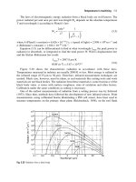
In this section, we present the effect of using different distances as the allocation

function for the dynamic clustering of a temperature dataset. The Dynamic Clus-
tering Algorithm (DCA) (Diday (1971)) represents a general reference for unsuper-
vised, not hierarchical and iterative, clustering algorithms. In particular, DCA simul-
taneously looks for the partition of the set of data and the representation of the clus-
ters. The main contributions to the clustering of interval data have been presented in
the framework of symbolic data analysis, especially for defining a way to represent
the clusters by means of prototypes (Chavent et al. (2006)). In the literature, several
authors indicate how to compute prototypes. In particular, Verde and Lauro (2000)
proposed that the prototype of a cluster must be considered as an element having
the same properties of the clustered elements. In such a way, a cluster of intervals
is described by a single prototypal interval, in the same way as a cluster of points is
represented by its barycenter.
Let E be a set of n data described by p interval variables X
j
( j = 1, ,p). The gen-
eral DCA looks for the partition P ∈ P
k
of E in k classes, among all the possible
partitions P
k
, and the vector L ∈ L
k
of k prototypes representing the classes in P,
such that, the following ' fitting criterion between L and P is minimized:
'(P
∗
,L
∗
)=Min{'(P,L) |P ∈P
k

,L ∈ L
k
}. (14)
Such a criterion is defined as the sum of dissimilarity or distance measures G(x
i
,G
h
)
of fitting between each object x
i
belonging to a class C
h
∈ P and the class represen-
tation G
h
∈ L:
'(P,L)=
k

h=1

x
i
∈C
h
G(x
i
,G
h
).

A prototype G
h
associated to a class C
h
is an element of the space of the description
of E, and it can be represented as a vector of intervals. The algorithm is initialized
by generating k random clusters or, alternatively, k random prototypes. Generally,
the criterion '(P,L ) is based on an additive distance on the p descriptors.
In the present paper, we present an application based on a dynamic clustering of a
real-world data set. The data set used in our experiments is the interval temperature
dataset shown in Table 1, which was previously used as a benchmark interval data
for cluster analysis in De Carvalho (2007), Guru and Kiranagi (2005) and Guru et
710 Rosanna Verde and Antonio Irpino
Table 1. The temperature dataset
City Jan Feb Mar Oct Nov Dec
Amsterdam [-4,4] [-5,3] [2,12] . . . [5,15] [-1,4] [-1,4]
Athens [6,12] [6,12] [8,16] . . . [16,23] [11,18] [8,14]
Bahrain [13,19] [14,19] [17,30] . . . [24,31] [20,26] [15,21]
Bombay [19,28] [19,28] [22,30] . [24,32] [24,30] [25,30]

Tokyo [0,9] [0,10] [3,13] . . . [13,21] [8,16] [2,12]
Toronto [-8,-1] [-8,-1] [-4,4] . . . [6,14] [-1,17] [-5,1]
Vienna [-2,1] [-1,3] [1,8] [7,13] [2,7] [1,3]
Zurich [-11,9] [-8,15] [-7,18] . . . [5,23] [0,19] [-11,8]
al. (2004). We performed a dynamic clustering using as the allocation function the
Hausdorff L
1
distance, the L
2
of De Carvalho et al. (2006), the De Carvalho adap-

tive distance (De Souza et al. (2004)) and the L
2
Wasserstein one alternatively. We
chose to obtain a partition into four clusters, and we compared the resulting par-
tition to that a priori one given by experts using the Corrected Rand Index. The
expert classification were the following (Guru et al. (2004)): Class 1 (Bahrain, Bom-
bay, Cairo, Calcutta, Colombo, Dubai, Hong Kong, Kula Lampur, Madras, Manila,
Mexico, Nairobi, New Delhi, Sidney); Class 2 (Amsterdam, Athens, Copenhagen,
Frankfurt, Geneva, Lisbon, London, Madrid, Moscow, Munich, New York, Paris,
Rome, San Francisco, Seoul, Stockholm, Tokyo, Toronto, Vienna, Zurich); Class 3
(Mauritius); Class 4 (Tehran).
Using the three different allocation functions, we obtained 3 optimal partitions
into 4 clusters (Tab.). 2). On the basis of the dynamic clustering, we evaluated the
obtained partitions with respect to the a priori ones using the Corrected Rand Indices
(Hubert and Arabie, (1985)).
5 Conclusion and perspectives
Interval descriptions can be derived from measurements subject to error (z ±e). If
they are assumed to be (probabilistic) models for the error term, Hausdorff distances
are not influenced by the distribution of values and the L
q
implicitly considers that
all the information is equally concentrated on the bounds of intervals. The Wasser-
stein distance permits the different position, variability and shape of the compared
distributions to be evaluated and taken separately into account, clearing way for inter-
preting data results. With a few modifications, it can also be used for the comparison
of two fuzzy numbers measured by LR fuzzy variables. Further, being an Euclidean
distance, it is easy to show that the Wasserstein distance satisfies the König-Huygens
theorem for the decomposition of inertia. This allows us to apply the usual indices
based on the comparison between the inter and the intra groups’ inertia for the eval-
uation and the interpretation of the results of a clustering or of a classification proce-

dure.
A New Interval Data Distance Based on the Wasserstein Metric 711
Table 2. Clusters obtained using different allocation functions. Last row: Corrected Rand In-
dex (CRI) of the obtained partition compared with the expert partition
c L
2
Wasserstein Adaptive L
2
Hausdorff L
1
distance
1
Bahrain Bombay Cairo Calcutta
Colombo Dubai HongKong
KulaLumpur Madras Manila
NewDelhi
Bahrain Bombay Calcutta Colombo
Dubai HongKong KulaLumpur
Madras Manila NewDelhi
Bahrain Dubai HongKong
NewDelhi Cairo MexicoCity
Nairobi
2
Amsterdam Copenhagen Frankfurt
Geneva London Moscow Munich
Paris Stockholm Toronto Vienna
Zurich
Amsterdam Copenhagen Frankfurt
Geneva London Moscow Munich
Paris Stockholm Toronto Vienna

Amsterdam Copenhagen Frankfurt
Geneva London Moscow Munich
Paris Stockholm Toronto Vienna
Zurich
3
Mauritius MexicoCity Nairobi
Sydney
Cairo Mauritius MexicoCity
Nairobi Sydney
Bombay Calcutta Colombo
KulaLumpur Madras Manila
Mauritius Sydney
4
Athens Lisbon Madrid New York
Rome SanFrancisco Seoul Tehran
Tokyo
Athens Lisbon Madrid New York
Rome SanFrancisco Seoul Tehran
Tokyo Zurich
Athens Lisbon Madrid NewYork
Rome SanFrancisco Seoul Tehran
Tokyo
CRI 0.53 0.49 0.46
On the other hand, a lot of effort is required for the extension of the distance to
the multivariate case. Indeed, here we just proposed an extension (in the sense of
Minkowski) of the distance under the hypothesis of independence between the de-
scriptors of a multidimensional interval datum.
References
BARRIO, E., MATRAN, C., RODRIGUEZ-RODRIGUEZ, J. and CUESTA-ALBERTOS,
J.A. (1999): Tests of goodness of fit based on the L2-Wasserstein distance. Annals of

Statistics , 27, 1230-1239.
COPPI, R., GIL, M.A., and KIERS, H.A.L. (2006): The fuzzy approach to statistical analysis.
Computational statistics and data analysis, 51, 1-14.
BOCK, H.H. and DIDAY, E., (2000): Analysis of Symbolic Data, Exploratory Methods for
Extracting Statistical Information from Complex Data. Springer-Verlag, Heidelberg.
CHAVENT, M., and LECHEVALLIER, Y. (2002): Dynamical clustering algorithm of interval
data: optimization of an adequacy criterion based on Hausdorff distance. In: Sokokowsky,
A.,BockH.H.(Eds.):Classification, Clustering and Data Analysis, Springer, Heidel-
berg, 53–59.
CHAVENT, M., DE CARVALHO, F.A.T., LECHEVALLIER, Y., and VERDE, R. (2006):
New clustering methods for interval data, Computational statistics, 21, 211–229.
DE CARVALHO, F.A.T. (2007): Fuzzy c-means clustering methods for symbolic interval
data.Pattern Recognition Letters, 28, 423–437
DE CARVALHO, F.A.T., BRITO, P., and BOCK, H. (2006): Dynamic clustering for interval
data based on L2 distance. Computational Statistics, 21, 2, 231-250
712 Rosanna Verde and Antonio Irpino
DE SOUZA, R. M. C. R. and DE CARVALHO, F. DE A. T. (2004): Clustering of Interval-
Valued Data Using Adaptive Squared Euclidean Distances. In Proc. of ICONIP 2004,
775-780.
DIDAY, E. (1971): La meéthode des Nueées dynamiques. Rev. Statist. Appl. 19 (2), 19–34.
GIBBS, A.L. and SU, F.E. (2002): On choosing and bounding probability metrics, Interna-
tional Statistical Review, 70, 419.
GURU, D. S. and KIRANAGI, B. B. (2005): Multivalued type dissimilarity measure and con-
cept of mutual dissimilarity value for clustering symbolic patterns. Pattern Recognition,
38, 1, 151-156.
GURU, D. S., KIRANAGI, B. B. and NAGABHUSHAN, P. (2004): Multivalued type prox-
imity measure and concept of mutual similarity value useful for clustering symbolic pat-
terns. Pattern Recognition Letters, 25, 10, 1203-1213.
HUBERT, L. and ARABIE, P. (1985): Comparing partitions. Journal of Classification, 2, 193–
218.

IRPINO, A. and ROMANO, E. (2007): Optimal histogram representation of large data
sets: Fisher vs piecewise linear approximations Revue des Nouvelles Technologies de
l’Information, RNTI-E-9, 99–110.
TRAN, L. and DUCKSTEIN, L. (2002): Comparison of fuzzy numbers using a fuzzy distance
measure, Fuzzy Sets and Systems, 130, 331–341.
VERDE, R. and LAURO, N. (2000): Basic choices and algorithms for symbolic objects dy-
namical clustering, in: XXXIIe Journées de Statistique,Fés, Maroc, Societé Française de
Statistique, 38–42.
Automatic Analysis of
Dewey Decimal Classification Notations
Ulrike Reiner
Verbundzentrale des Gemeinsamen Bibliotheksverbundes (VZG)
37077 Göttingen, Germany

Abstract. The Dewey Decimal Classification (DDC) was conceived by Melvil Dewey in
1873 and published in 1876. Nowadays, the DDC serves as a library classification system in
about 138 countries worldwide. Recently, the German translation of the DDC was launched,
and since then the interest in DDC has rapidly increased in German-speaking countries. The
complex DDC system (Ed. 22) allows to synthesize (to build) a huge amount of DDC no-
tations (numbers) with the aid of instructions. Since the meaning of built DDC numbers is
not obvious – especially to non-DDC experts – a computer program has been written that au-
tomatically analyzes DDC numbers. Based on Songqiao Liu’s dissertation (Liu (1993)), our
program decomposes DDC notations from the main class 700 (as one of the ten main classes).
In addition, our program analyzes notations from all ten classes and determines the meaning
of every semantic atom contained in a built DDC notation. The extracted DDC atoms can be
used for information retrieval, automatic classification, or other purposes.
1 Introduction
While searching for books, journals, or web resources, you will often come across
numbers such as "025.1740973", "016.02092", or "720.7073". What do they mean?
Librarian professionals will identify these strings as numbers (notations) of the

Dewey Decimal Classification (DDC), which is named after its creator, Melvil Dewey.
Originally, Dewey designed the classification for libraries, but in the meantime DDC
has also been discovered for classifying the web or other resources. The DDC is used,
among others, because it has a long-standing tradition and is still up to date: in order
to cope with scientific progress, it is currently under development by a ten-member
international board (the Editorial Policy Committee, EPC). While the first edition,
which was published in 1876, only comprised a few pages, the current 22nd edition
of the DDC spans a four-volume work with almost 4,000 pages. Today, the DDC
contains approx. 48,000 DDC notations and about 8,000 instructions. The DDC no-
tations are enumerated in the schedules and tables of the DDC. With the aid of the
instructions mentioned above, human classifiers can build new synthesized notations
(numbers) if these are not specifically listed in the DDC schedules. This way, an
enormous amount of synthesized DDC notations has been built intellectually over
698 Ulrike Reiner
the last 130 years. These mostly unused notations are contained in library catalogues
– like a hidden treasure. They can be considered as belonging to the "Deep Lib", one
of the subsets of the "Deep Web" (Bergman (2001)). Can these notations be made
accessible for information retrieval purposes with reasonable effort?
Our answer to this question consists in the automatic analysis of notations of the
DDC. The analysis program we have developed determines all DDC notations (to-
gether with their corresponding captions) contained in a synthesized (built) DDC
notation. Before we go into details of the automatic analysis of DDC notations in
section 3, section 2 provides the basis for the analysis. In section 4, the results are
presented, and section 5 draws a conclusion.
2 DDC notations
Notations play an important role in the DDC:
"Notation is the system of symbols used to represent the classes in a classifica-
tion system. The notation provides a universal language to identify the class and
related classes, regardless of the fact that different words or languages may be used
to describe the class." ( />The following picture serves as an example for the aforesaid. Class C is rep-

resented by the notation 025.43 or, respectively, by the captions of three different
languages:
025.43
❳
❳
❳
❳
❳
❳
❳③
Universalklassifikationssysteme ✲
General classification systems ✲
Système de classification ✘
✘
✘
✘
✘
✘
✘✿
class C
✫✪
✬✩
Fig. 1. Class C represented by notation 025.43 or by several captions
In compliance with the DDC system, the automatic analysis of notations of the
DDC is carried out in the VZG (VerbundZentrale des Gemeinsamen Bibliotheksver-
bundes) project Colibri (COntext generation and LInguistic tools for Bibliographic
Retrieval Interfaces). The goal of this project is to enrich title records on the basis of
the DDC to improve retrieval. The analysis of DDC notations is conducted under the
following research questions (which are also posed in a similar way in Liu (1993),
p. 18): Q1. Is it possible to automatically decompose molecular DDC notations into

Automatic Analysis of Dewey Decimal Classification Notations 699
atomic DDC notations? Q2. Is it possible to improve automatic classification and
retrieval by means of atomic DDC notations? An atomic DDC notation is a semanti-
cally indecomposable string (of symbols) that represents a DDC class. A molecular
DDC notation is a string that is syntactically decomposable into atomic DDC nota-
tions.
DDC notations can be found at several places in the DDC. In DDC summaries,
the notations for the main classes (or tens), the divisions (or hundreds), and the
sections (or thousands) are enumerated. Other notations are listed in the schedules
("DDC schedule notations") or tables ("DDC table notations") or internal tables.
DDC schedules are "the series of DDC numbers 000-999, their headings (captions),
and notes." (Mitchell (1996), p. lxv). A DDC table is "a table of numbers that may be
added to other numbers to make a class number appropriately specific to the work be-
ing classified" (Mitchell (1996), p. lxv). Further notations are contained in the "Rel-
ative Index" of the DDC. The frequency distributions of schedule (table) notations
are shown in Fig. 2 (Fig. 3), while schedno0 is short hand for DDC schedule nota-
tions beginning with 0, schedno1 for DDC schedule notations beginning with 1, etc.
The captions for the main classes are: 000: Computer science, information & gen-
eral works; 100: Philosophy & psychology; 200: Religion; 300: Social sciences; 400:
Language; 500: Science; 600: Technology; 700: Arts & recreation; 800: Literature;
900: History & geography. As illustrated by Fig. 2, DDC notations are not distributed
uniformly: the most schedule notations can be found in the class "Technology", fol-
lowed by the notations in the class "Social sciences". The fewest notations belong
to the class "Philosophy & psychology". With regard to the table notations (Fig. 3),
the 7,816 Table 2 notations ("Geographic Areas, Historical Periods, Persons") stand
out, whereas, in contrast, the quantities of all other table notations are comparatively
small (Table 1: Standard Subdivisions; Table 3: Subdivisions for the Arts, for Indi-
vidual Literatures, for Specific Literary Forms; Table 4: Subdivisions of Individual
Languages and Language Families; Table 5: Ethnic and National Groups; Table 6:
Languages).

As mentioned before, DDC notations that are not explicitly listed in the schedules
can be built by using DDC instructions. This process is called "notational synthesis"
or "number building". Its results are synthesized DDC notations (molecular DDC
notations) that usually only DDC experts are able to interpret. But with the aid of
our computer program "DDC analyzer", the meaning of molecular DDC notations
is revealed and the determined atomic DDC notations can be used, among others, to
answer question Q2.
3 Automatic analysis of DDC notations
The GBV Union Catalog GVK (Gemeinsamer VerbundKatalog, http://gso.
gbv.de/) contains 3,073,423 intellectually DDC-classified title records (status: July,
2004). After the automatic elimination of segmentation marks, obviously incorrect
DDC notations (3.8 per cent of all DDC notations), and duplicate DDC notations, a
total of 466,134 different DDC notations is available for the automatic analysis of
700 Ulrike Reiner
Fig. 2. Frequency distribution of DDC schedule notations
Fig. 3. Frequency distribution of DDC table notations
DDC notations. This set of all GVK DDC notations serves as input data for the DDC
analyzer. The frequency of DDC schedule notations is as follows (in descending
order): those beginning with 3 (189,246), with 9 (62,115), with 7 (52,632), with 6
(51,704), with 5 (33,649), with 0 (23,946), with 2 (20,888), with 8 (20,678), with 4
(6,680), and with 1 (4,596). The arity of DDC notations of all GVK DDC notations
Automatic Analysis of Dewey Decimal Classification Notations 701
is Gaussian distributed with a maximum at 10, i.e. most DDC notations have approx.
arity 10, the shortest DDC notation has arity 1, the longest DDC notation has arity
29. Other important input data for the DDC analyzer we used were the 600 DDC
numbers given in Liu’s dissertation. These 600 DDC numbers that we call "Liu’s
sample" were randomly selected from class 700 from the OCLC database by Liu.
As a member of the Consortium DDC German, we have access to the machine-
readable data of the 22nd edition of the DDC system. These data are stored in an xml
file. The English electronic web version is available as WebDewey

( the German pendant as MelvilClass (-
deutsch.de/melvilclass-login). For our purpose, only the relevant data of the xml file,
which contains the expert knowledge of the DDC system, are extracted and stored
in a "knowledge base". Here, DDC notations, descriptors, and descriptor values are
stored in consecutive fields, while facts and rules – as we call them – are represented
in a very similar way:
T1–093-T1–099+021#<ba4r2>#Statistics
025.17#<na1r1>##025.17#025.341-025.349#025.34#####
025.344#<hat>#Electronic resources
The three example lines of the knowledge base should be read as follows: Fact:
T1–093-T1–099+021 has the caption "Statistics". Rule: Add to base number 025.17
the numbers following 025.34 in 025.341-025.349. Fact: 025.344 has the caption
"Electronic resources". ’#’ serves as field separator. The xml tags that are given in
angle brackets stand for: "ba4" ("beginning of add table (all of table number)"), "na1"
("add note (part of schedule number)") and "hat" ("hierarchy at class"). "r1" and "r2",
which follow "na1" or, respectively, "ba4", stand for the first two macro rules. The
knowledge base contains 48,067 facts and 8,033 rules. The 8,033 rules can be gener-
alized to macro rules. While Liu (1993) defined 17 (macro) rules for the decomposi-
tion for class 700, we defined 25 macro rules for all DDC classes.
Our program, the DDC analyzer, works as follows: after initializing variables, it
reads the knowledge base and, triggered by one or more DDC notations to be an-
alyzed, executes the analysis algorithm. The number of correct and incorrect DDC
notations is counted. For a DDC notation, there are two phases to the analyzing pro-
cess including: determining the facts from left to right (phase 1) and determining
the facts via rules from left to right (phase 2). After checking which output for-
mat has to be printed, the result is printed as a DDC analysis diagram or as a DDC
analysis result set. After all DDC notations have been analyzed, the number of to-
tally/partially analyzed DDC notations is printed. There are different reasons for a
partially analyzed DDC notation: either the implementation of the DDC analyzer is
incorrect/incomplete or the DDC notation is incorrectly synthesized or a part of the

DDC system itself is incorrect.
702 Ulrike Reiner
4 Results
To demonstrate our progress in comparison with Liu’s work, we compare his decom-
position result with our DDC analysis diagram for the 37th molecular DDC notation
of his sample:
Liu (1993), pp. 99–100
720.7073 has been decomposed as follows:
720: Architecture
0707: Geographical treatment
73: United States
The title of this book is:
#aVoices in architectural education: #bcultural politics and
The subject headings for this book are:
#aArchitecture #xStudy and teaching #zUnited States.
#aArchitecture and state #zUnited States.
Reiner (2007a),p.49
720.7073
<liu_37_to_analyze; length: 8>
7
Arts & recreation <hatzen>
72
Architecture <hatzen>
720
Architecture <hat>
-0.7
Education, research, related topics <T1–07>
-0.707-
Geographic treatment <T1–0707>
7-

North America <na4r7span:T1–0701-T1–0709:T2–7>
73
United States <na4r7span:T1–0701-T1–0709:T2–73>
The information given in angle brackets should be read as follows: "hatzen" is the
concatenation of "hat" ("hierarchy at class") and "zen" ("zen built entry (main tag)").
"T1–" stands for "table 1", "T2–" for "table 2", "na4" for "add note (add of table
number)", "r7" for "macro rule 7", "span" for "span of numbers", and ":" for "delim-
iter". As you can see, while Liu decomposes the synthesized DDC notation into three
chunks, our DDC analysis diagram shows the finest possible analysis of the molecu-
lar DDC notation. The fine analysis provides the advantage of uncovering additional
captions: "Arts & recreation", "Architecture", "North America", and "Education, re-
search, related topics".
A DDC analysis diagram contains analysis and synthesis information: 1. the
molecular DDC notation to be analyzed; 2. an identifier (name) and the length of
the molecular DDC notation; 3. the sequence and position of the digits within the
molecular DDC notation; 4. the Dewey dot at position 4; 5. the relevant parts of
the molecular DDC notation for each analysis step; 6. the corresponding caption for
every atomic DDC notation; 7. the parts irrelevant for the respective analysis step
marked with "-"; 8. the type of the applied facts and rules that appear in angle brack-
ets. In case it has been explained how to read the given information mentioned in 8.,
every synthesis step can be reproduced. While DDC analysis diagrams are intended
for human experts, the DDC analysis result set can be used for data transfer. Cur-
Automatic Analysis of Dewey Decimal Classification Notations 703
rently, we distinguish three kinds of analysis result sets. The first one is a set of DDC
<notation;caption> tuples:
7;Arts & recreation
72;Architecture
720;Architecture
T1–07;Education, research, related topics
T1–0707;Geographic treatment

T2–7;North America
T2–73;United States
The second one delivers all DDC notations contained in a synthesized number:
liu_37:720.7073;7;72;720;T1
-
07;T1
-
0707;T2
-
7;T2
-
73
The third analysis result set is in MAB2 format:
705a
ˆ
_a720.7073
ˆ
_p72
ˆ
_cT1–070
ˆ
_f0707
ˆ
_g73
All 600 analyzed DDC notations of Liu’s sample have been compared accordingly
with the results of Liu (1993). It turns out that Liu’s decompositions can be repro-
duced. Minor differences result from printing errors in his dissertation and the usage
of different (20th/22nd) DDC editions. After 14 years, 36 DDC notations of Liu’s
sample are out of date because of relocations and discontinuations. As far as the
analysis of the 466,134 GVK DDC notations of all DDC classes is concerned, cur-

rently 297,782 (168,352) DDC notations can be totally (partially) analyzed, i.e. 63.9
per cent (36.1 per cent) are totally (partially) analyzed. In some DDC classes, the
analyzing degree is even higher, which means that, e.g., 87 per cent of the 51,704
DDC notations of the class "Technology" (600) can be totally analyzed.
5 Conclusion
In 1993, Liu showed that DDC synthesized class numbers of main class 700 can
be decomposed automatically. Our program analyzes notations from all ten main
classes. Compared to Liu’s approach, our analysis procedure delivers more infor-
mation, which is furthermore presented in a new way. Since Liu’s expert-evaluated
results are reproduced, we can (statistically) infer that our DDC analyzer works cor-
rectly with high probability. Increasing the quantity of DDC notations totally ana-
lyzed will be the next step. The results can be used to improve (multilingual) DDC
information retrieval or DDC automatic classification systems. On the basis of analy-
sis diagrams, DDC tutorials or expert systems could be developed to support teaching
of DDC number building or to control the quality of built DDC numbers.
704 Ulrike Reiner
References
BERGMAN, M., K.: The Deep Web: Surfacing Hidden Value. The Journal of Electronic
Publishing, Volume 7, Issue 1, August 2001. Online: />01/bergman.html
MITCHELL, J.,S. (ed.) (1996): Dewey Decimal Classification and Relative Index. Ed.
21, Volumes 1-4. Forest Press, OCLC, Inc., Albany, New York, 1996. (http://connex
ion.oclc.org/).
LIU, S. (1993): The Automatic Decomposition of DDC Synthesized Numbers. Ph.D. diss., Uni-
versity of California, Graduate School of Library and Information Science, Los Angeles,
1993.
REINER, U. (2005): VZG-Projekt Colibri – DDC-Notationsanalyse und -synthese. September
2004 - Februar 2005. VZG-Colibri-Bericht 2/2004. Verbundzentrale des Gemeinsamen
Bibliotheksverbundes (VZG), Göttingen, 2005.
REINER, U. (2007a): Automatische Analyse von Notationen der Dewey-Dezi-
malklassifikation. 31st Annual Conference of the German Classification Society

on Data Analysis, Machine Learning, and Applications – Librarian Workshop:
Subject Indexing and Library Science. March 7-9, 2007, Freiburg i. Br., Germany.
( />REINER, U. (2007b): Automatische Analyse von DDC-Notationen und DDC-Klassifizierung
von GVK-Plus-Titeldatensätzen. Workshop zur Dewey-Dezimalklassifikation "DDC-
-Einsichten und -Aussichten 2007". March 1, 2007, SUB Göttingen, Germany.
( />Effects of Data Transformation on Cluster Analysis of
Archaeometric Data
Hans-Joachim Mucha
1
, Hans-Georg Bartel
2
and Jens Dolata
3
1
Weierstraß-Institut für Angewandte Analysis und Stochastik (WIAS),
Mohrenstraße 39, 10117 Berlin, Germany

2
Institut für Chemie, Humboldt-Universität zu Berlin,
Brook-Taylor-Straße 2, 12489 Berlin, Germany

3
Landesamt für Denkmalpflege Rheinland-Pfalz, Abt. Archäologie, Amt Mainz,
Große Langgasse 29, 55116 Mainz, Germany

Abstract. In archaeometry the focus is mainly on chemical analysis of archaeological arti-
facts such as glass objects or pottery. Usually the artefacts are characterized by their chemical
composition. Here the focus is on cluster analysis of compositional data. Using Euclidean
distances cluster analysis is closely related to principal component analysis (PCA) that is
a frequently used multivariate projection technique in archaeometry. Since PCA and cluster

analysis based on Euclidean distances are scale dependent, some kind of "appropriate" data
transformation is necessary. Some different techniques of data preparation will be presented.
We consider the log-ratio transformation of Aitchison and the transformation into ranks in
more detail. From the statistical point of view the latter is a robust method.
1 Introduction
Often the archaeometric data we analyze are measured with respect to the chemical
compositions of many variables that usually have quite different scales. For example,
Mucha et al. (2001) investigated a data set of ancient coarse ceramics by cluster
analysis, where the set of 19 variables consists of nine oxides and ten trace elements
(see below Section 6). The former are given in percent and the latter are measured in
parts per million (ppm). Hence some kind of treatment of the data is necessary since
PCA and cluster analysis based on Euclidean distances are scale dependent. Without
some standardization, the Euclidean distances can be fully dominated by the variable
in the more sensitive units. However, as we will see below, an inappropriate data
transformation can result in covering the differences between well-separated groups
(clusters). Moreover it can produce outliers.
Besides different scales of the variables, often problems with outliers and with
long-tailed (skew) distributions of the variables were addressed in the archaeometric
682 Hans-Joachim Mucha, Hans-Georg Bartel and Jens Dolata
data, see recently Baxter (2006). Figure 1 shows an example taken from Baxter and
Freestone (2006) (see also below Section 5). This is discrete data rather than metric
data: the measurements are given as 0.01, 0.02 and so on. The usual way of dealing
with outliers seems to be omitting them, see for instance Baxter (2006) and Bax-
ter and Freestone (2006). Another more objective way is using transformation into
ranks, as it will be shown below.
Fig. 1. The frequency plot of MnO of 80 objects shows a skew density. Additionally, at the
bottom the corresponding rank values are shown.
Indeed, the performance of multivariate statistical methods like cluster analysis
and PCA is often seriously affected by these two main problems: scale dependence
and outliers. Concerning PCA see Baxter (1995) and Baxter and Freestone (2006).

Therefore data transformations and outlier treatment are highly recommended by
these authors.
Here different data transformations will be presented and compared. Our inves-
tigation shows that especially nonparametric transformations like the transformation
of the data into a matrix of ranks for subsequent multivariate statistical analysis give
good and for archaeologists reasonable results. We consider two data sets: the com-
positional data of colourless Romano-British vessel glass where the variables mea-
sured sum to 100%, and the sub-compositional data of Roman bricks and tiles from
the Rhine area where the variables measured sum to approximately 100%.
2 Data transformation in archaeometry
Let I objects x
i
be on hand for J variables. That is, a data matrix X =(x
ij
) with
elements x
ij
≥ 0 is under investigation. For compositional data, Aitchison (1986)
recommended the log-ratio transformation
y
ij
= log(x
ij
/g(x
i
)) ,(1)
Data Transformation in Archaeometry 683
where g(x
i
)=(x

i1
x
i2
x
iJ
)
1/J
is the geometric mean of the ith object. This trans-
formation is restricted to values x
ij
> 0. Baxter and Freestone (2006) criticized that
Aitchison argued that all others transformations are "meaningless" and "inappropri-
ate" for compositional data. The authors presented the failure of PCA for different
data sets based on the log-ratio transformation. In Section 5 below the failure of
cluster analysis methods based on the log-ratio transformation will be presented.
The transformation of the variables by
y
ij
=(x
ij
−x
j
)/s
j
(2)
is known as standardization. Herein
x
j
and s
j

are the mean and standard deviation of
variable j, respectively. The new variables y
j
has mean equals 0 and variance equals
1. The logarithmic transformations
y
ij
= log(x
ij
) (3)
or
y
ij
= log(x
ij
+ 1) (4)
can handle skew densities, where (3) is restricted to values x
ij
> 0, as the log-ratio
transformation (1). Here the meaning of differences is changed.
3 Transformation into ranks
The multivariate statistical analysis based on ranks rather than based on the original
data solves the problems of different scales and skewness. The influence of outliers
is removed in the univariate case. In the multivariate case, the influence of outliers
is highly reduced usually but theoretically the problem of outliers remains to some
degree (Rohatch et al. (2006)).
Table 1. Measurements and the corresponding ranks of MnO
Value 0.01 0.02 0.03 0.04 0.05 0.06 0.07 0.08 0.09 0.10 0.11 0.13
Frequency171820715423111
Rank 9 26.5 45.5 59 63 66 70.5 73.5 76 78 79 80

Transformation into ranks is quite simple: one replaces the measurements by
their ranks 1,2, ,I where I is the number of observations. The mean of each of
the new rank order variables become the same: (I +1)/2. Moreover, the variance of
each of the new variables become the same: (I
2
−1)/12. In case of multiple values
we recommend to average the corresponding ranks (Figure 1). Table 1 contains both
the original values and the ranks of MnO of the 80 objects (see also Figure 1, data
source: Baxter and Freestone (2006)).
Mucha (1992) presented a successful application of partitioning cluster analysis
based on rank data. Also, Mucha (2007) investigated the stability of hierarchical
clustering based on rank data. The aim of this paper here is to show that cluster
analysis based on rank data gives good results and that it can outperform log-ratio
cluster analysis.
684 Hans-Joachim Mucha, Hans-Georg Bartel and Jens Dolata
Fig. 2. PCA plot of groups of Romano-British vessel glass based on ranks (left hand side), and
PCA plot of group membership based on log-ratio transformed data (right).
Fig. 3. Fingerprint of the true Euclidean distances of rank data (left) and of log-ratio trans-
formed data (right). (Small distances are marked by dark gray, great distances by light gray.)
4 Distances and cluster analysis
Henceforth let us focus on the squared Euclidean distances in cluster analysis be-
cause PCA is based on the same distance measure and the PCA plots are very pop-
ular in archaeometry (Baxter (1995), Baxter and Freestone (2006)). Cluster analysis
and PCA are multivariate statistical methods that are based on distance measures.
Further let us restrict to the well-known hierarchical Ward’s method (Späth (1985)).
It is the simplest of the model-based Gaussian clustering methods that are applied by
Papageorgiou et al. (2002) for finding groups of artefacts.
Data Transformation in Archaeometry 685
In case of the log-ratio transformation (1) the squared Euclidean distance be-
tween two objects i and h is

d(x
i
,x
h
)=
J

j=1
(y
ij
−y
ih
)
2
=
J

j=1
(log
x
ij
g(x
i
)
−log
x
hj
g(x
h
)

)
2
. (5)
Often it is called Aitchison distance. Appropriate clustering techniques for squared
Euclidean distances are the the partitioning K-means method (Mucha (1992)) and
the hierarchical Ward’s method, as mentioned already above.
5 Romano-British vessel glass classified
This is simulated data based on real data of colourless Romano-British vessel glass
(Baxter et al. (2005)). Details and the complete source can be taken from Baxter and
Freestone (2006). This example is based on two groups that are well-known different.
Group 1 consists of 40 cast bowls with high amounts of Fe
2
O
3
. Group 2 also
consists of 40 objects: this is a collection of facet-cut beakers with low Al
2
O
3
.In
Figure 2 at the left hand side, the two groups are shown in the first plane of the PCA
based on rank data. This projection gives a good approximation of the distances
between objects. Axis 1 (39%) and axis 2 (20%) are highly significant (see Lebart et
al. (1984) for tables of significance of eigenvalues of PCA). The Ward’s method finds
the true groups without any error. The same optimum clustering result is obtained
when using the transformation (4).
In Figure 2 at the right hand side, the two groups are presented by the PCA plot
after the data transformation by (1). This transformation produces outliers such as
the object 79 that is drawn additionally. The PCA is based on the Aitchison distance
measure (5). In the two-dimensional projection the distances are approximative ones.

The Ward’s method never finds the true two groups. Table 2 at the left hand side
shows the very low correspondence between the given groups and the clusters found.
The same bad cluster analysis result is obtained when using the transformation (3).
The transformation (2) performs here much better: the Ward’s method results in 5
errors only (see Table 2 at the right hand side). The corresponding PCA-plot of the
standardized data using (2) is published as Figure 8 by Baxter and Freestone (2006).
There is no outlier in this plot as well as in the plot of Figure 2 at the left hand side.
Table 2. True groups versus clusters
True Ward’s method with (1) Ward ’s method with (2)
Groups Cluster 1 Cluster 2 Cluster 1 Cluster 2
Cast bowls 27 9373
Facet-cut beakers 33 8238
Figure 3 compares two fingerprints of the Euclidean distances of rank data (left
hand side) and of log-ratio transformed data (right), respectively. Here the objects are
686 Hans-Joachim Mucha, Hans-Georg Bartel and Jens Dolata
sorted first by group and then within the group by the first principal component based
on rank analysis and by the first principal component based on log-ratio scaling,
respectively. The fingerprint at the right hand side shows no clear class structure.
Additionally, the outlier 79 is marked at the bottom. The corresponding high distance
values to all the remaining objects build the eye-catching column and row in light
gray, respectively.
Fig. 4. PCA plot of group membership based on rank data.
6 Roman bricks and tiles classified
Roman bricks and tiles from the Rhine area are described by 19 chemical elements
that were measured using X-Ray Fluorescence Analysis (XRF). All the chemical
measurements were performed by G. Schneider of the Freie Universität Berlin. Two
well-known locations of production are Groß-Krotzenburg and Straßburg-Königshofen
(Dolata (2000)). In this reference the author published the complete data source. It
is possible to confirm the two well-known groups by cluster analysis based on rank
data?

Figure 4 shows the PCA plot of the two groups based on rank data. The hierar-
chical Ward’s method method finds the true groups without any error.
In Figure 5 the two groups are shown by the PCA projection based on the data
transformation (1). Here Ward’s method finds the groups but one error occurs: the
outlier at the bottom at the left hand side coming from Straßburg-Königshofen is
misclassified.
Data Transformation in Archaeometry 687
Fig. 5. PCA plot of group membership based on log-ratio transformed data.
7 Summary
There are different data transformations in use in archaeometry with advantages and
disadvantages. Comparison of different data transformations based on simulated and
real data shows that transformation into ranks is useful in the case of outliers and
skew densities. However, most of the quantitative information is lost by going to
ranks. From archaeological point of view rank analysis gives reasonable results.
Other transformations (like Aitchison
´
Ss log-ratio or (3)) are highly affected by out-
liers, skew densities and values near 0. Therefore finding the true groups by cluster
analysis fails in the case of glass data. Moreover, new artificial outliers can be pro-
duced by transformations such as (1) and (3) in case of measurements near zero.
References
AITCHISON, J. (1986): The Statistical Analysis of Compositional Data. Chapman and Hall,
London.
BAXTER, M. J. (1995): Standardization and Transformation in Principal Component Analy-
sis, with Applications to Archaeometry. Applied Statistics, 44, 513–527.
BAXTER, M. J. (2006): A Review of Supervised and Unsupervised Pattern Recognition in
Archaeometry. Archaeometry, 48, 671–694.
BAXTER, M. J. and FREESTONE, I. C. (2006): Log-ratio Compositional Data Analysis in
Archaeometry. Archaeometry, 48, 511–531.
688 Hans-Joachim Mucha, Hans-Georg Bartel and Jens Dolata

BAXTER, M. J., COOL, H. E. M., and JACKSON, C. M. (2005): Further Studies in the
Compositional Variability of Colourless Romano-British Vessel Glass. Archaeometry, 47,
47–68.
DOLATA, J. (2000): Römische Ziegelstempel aus Mainz und dem nördlichen Ober-germanien
- Archäologische und archäometrische Untersuchungen zu chrono-logischem und
baugeschichtlichem Quellenmaterial. Inauguraldissertation, Johann Wolfgang Goethe-
Universität, Frankfurt/Main.
LEBART, L., MORINEAU, A. and WARWICK, K. M. (1984): Multivariate Descriptive Sta-
tistical Analysis. Wiley, New York.
MUCHA, H J. (1992): Clusteranalyse mit Mikrocomputern. Akademie Verlag, Berlin.
MUCHA, H J. (2007): On Validation of Hierarchical Clustering. In: R. Decker and H J.
Lenz (Eds.): Advances in Data Analysis, Springer, Berlin, 115–122.
MUCHA, H J., DOLATA, J., and BARTEL, H G. (2001): Validation of Results of Cluster
Analysis of Roman Bricks and Tiles. In: W. Gaul and G. Ritter (Eds.): Classification,
Automation, and New Media. Springer, Berlin, 471–478.
PAPAGEORGIOU, I., BAXTER, M. J., and CAU, M. A. (2001): Model-based Cluster Anal-
ysis of Artefact Compositional Data. Archaeometry, 43, 571–588.
ROHATCH, T., PÖPPEL, G., and WERNER, H. (2006): Projection Pursuit for Analyzing
Data From Semiconductor Environments. IEEE Transactions on Semiconductor Manu-
facturing, 19, 87–94.
SPÄTH, H. (1985): Cluster Dissection and Analysis. Ellis Horwood, Chichester.
Fuzzy PLS Path Modeling: A New Tool For Handling
Sensory Data
Francesco Palumbo
1
, Rosaria Romano
2
and Vincenzo Esposito Vinzi
3
1

University of Macerata, Italy

2
University of Copenhagen, Denmark

3
ESSEC Business School of Paris, France

Abstract. In sensory analysis a panel of assessors gives scores to blocks of sensory attributes
for profiling products, thus yielding a three-way table crossing assessors, attributes and prod-
ucts. In this context, it is important to evaluate the panel performance as well as to synthesize
the scores into a global assessment to investigate differences between products. Recently, a
combined approach of fuzzy regression and PLS path modeling has been proposed. Fuzzy
regression considers crisp/fuzzy variables and identifies a set of fuzzy parameters using op-
timization techniques. In this framework, the present work aims to show the advantages of
fuzzy PLS path modeling in the context of sensory analysis.
1 Introduction
In sensory analysis a panel of assessors gives scores to blocks of sensory attributes
for profiling products, thus yielding a three-way table crossing assessors, attributes
and products. This type of data are characterized by three different sources of com-
plexity: complex structure of relations among the variables (different blocks), three
directions of information (samples, assessors, attributes) and influential human be-
ings’ involvement (assessors’ evaluations).
Structural Equation Models (SEM) (Bollen, 1989) consist of a network of causal
relationships among Latent Variables (LV) defined by blocks of Manifest Variables
(MV). The main idea behind SEM is that the features on which the analysis would fo-
cus cannot be properly measured and are determined through the measured variables.
In a recent contribution (Tenenhaus and Esposito-Vinzi, 2005), SEM have been suc-
cessfully used to analyze sensory data. When SEM are based on the scores of a set
of assessors, they are generally based on the mean scores. However, it is important

to analyze if there exist individual differences between assessors. Even if assessors
are carefully trained to adopt the same yardstick, this cannot completely protect us
against their single sensibility.
690 Palumbo et al.
When human estimation is influential and the observations cannot be described
accurately but we can give only an approximate description of them, fuzzy approach
is more useful and convenient than the classical one (Zadeh, 1965). Fuzzy sets al-
low us coding and treating many different kinds of imprecise data. Recently, a fuzzy
approach to SEM has been proposed (Romano, 2006) and successively used for com-
paring different SEM (Romano and Palumbo, 2006b).
The present paper proposes to use the new fuzzy structural equation models for
handling the different sources of information and uncertainty arising from sensory
data. First a brief introduction to the methodology of reference (Romano, 2006) will
be given. Then an application to data from sensory profiling will be presented.
2 Fuzzy PLS path modeling
Fuzzy PLS Path Modeling is a new methodology to dealing with system complexity.
It allows us taking into account both complexity in information codification and in
structures of relations among the variables. Fuzzy codification and structural equa-
tions are combined to handling these different sources of complexity, respectively.
The strategy allowing imprecision in codification for reducing complexity is ap-
propriately expressed by Zadeh’s principle of incompatibility (Zadeh, 1973). The
main idea is that the traditional techniques for analyzing systems are not well suited
to dealing with human systems. In human thinking, the key elements are not numbers
but classes of objects or concepts in which the membership of each element to the
class is gradual (fuzzy) rather than sharp. For instance, the concept of sweet coffee
does not correspond to an exact amount of sugar in the coffee. But it is possible to
define the classes sweet coffee, normal coffee, bitter coffee.
On the other hand, the descriptive complexity of a system can also be reduced by
breaking the system into its appropriate subsystems. This is the general principle
behind Structural Equation Models (SEM) (Bollen, 1989). The basic idea is that dif-

ferent subsets of variables are the expression of different concepts, belonging to the
same phenomenon. These concepts are named latent variables (LV) as they are not
directly observable but measurable by means of a set of manifest variables (MV).
The aim of SEM is to study the system of relations between each LV and its MV, and
among the different LV inside the system. Considering one by one each part forming
the whole system, and analyzing the relations among the different parts, the system
complexity is reduced allowing a better description of the main system characteris-
tics.
F-PLSPM consists in introducing fuzzy models inside SEM, by means of a two-
stage procedure. This allows dealing with system complexity using both an approach
which is tolerant to imprecision and a well suited methodology to link the different
parts into which the system may be decomposed.
2.1 Interval data, fuzzy data and fuzzy models
It is very common to measure statistical variables in terms of single-values. How-
ever, for many reasons, and in many situations exact measures are very hard (or even
Fuzzy PLS Path Modeling 691
impossible) to achieve.
A rigorous study of interval data is given by Interval Analysis (Alefeld and Herzen-
berger, 1987). In this framework, an interval value is a bounded subset of real num-
bers [x]=[x
,x], formally:
[x]={x ∈ R| x
≤ x ≤ x} (1)
where x
and x are called lower and upper bound, respectively. Alternatively, an in-
terval value may by expressed in terms of width (or radius), x
w
,andcenter (or mid-
point), x
c

: x
w
=
1
2
|x −x| and x
c
=
1
2
|x + x|.
A fuzzy set is a codification of the information allowing us to represent vague
concepts expressed in natural language. Formally, given the universe of objects :, Z
as the generic element, a fuzzy set
˜
A in : is defined as a set of ordered pairs:
˜
A = {(Z,z
˜
A
(Z))|Z ∈ :} (2)
where the value z
˜
A
(Z
0
) expresses the membership degree for a generic element Z
0
∈
:. The larger the value of z

˜
A
(Z), the higher the degree of membership of Z in
˜
A.If
the membership function is permitted to have only the values 0 and 1 then the fuzzy
set is reduced to a classical crisp set. The universal set : may consist of discrete
(ordered and non ordered) objects or it can be a continuous space.
A fuzzy set in the real line that satisfies both the conditions of normality and
convexity is a fuzzy number.
It must be normal so that the statement “real number close to r" is fully satisfied by r
itself, i.e. z
˜
A
(r)=1. In addition, all its D−cuts for D ≡0 must be closed intervals so
that the arithmetic operations on fuzzy sets can be defined in terms of operations on
closed intervals. On the other hand, if all its D−cuts are closed intervals, it follows
that the fuzzy number is a convex fuzzy set.
In possibility theory (Zadeh, 1978), a branch of fuzzy set theory, fuzzy numbers are
described by possibility distributions.
A possibility distribution S
˜
A
(Z) is a function which satisfies the following condi-
tions (Tanaka and Guo, 1999): i) there exists an Z such that S
˜
A
(Z)=1 (normality);
ii) D−cuts of fuzzy numbers are convex; iii) S
˜

A
(Z) is piecewise continuous.
Particular fuzzy numbers are the symmetrical fuzzy numbers whose possibility dis-
tribution may be denoted as:
S
˜
A
i
(Z)=max

0,1 −




Z −c
i
r
i




q

(3)
Specifically, (3) corresponds to triangular fuzzy numbers when q = 1, to square root
fuzzy numbers when q = 1/2andparabolic fuzzy numbers when q = 2. It is easy to
show that (3) corresponds to intervals when q =+f.
It is worth noticing that fuzzy variables are associated with possibility distributions

in the similar way that random variables are associated with probability distributions.
Furthermore, possibility distributions are numerically equal to membership functions
(Zadeh, 1978).