- Trang chủ >>
- Khoa Học Tự Nhiên >>
- Vật lý
Short-Wave Solar Radiation in the Earth’s Atmosphere Part 2 ppsx
Bạn đang xem bản rút gọn của tài liệu. Xem và tải ngay bản đầy đủ của tài liệu tại đây (388.75 KB, 32 trang )
20 Solar Radiation in the Atmosphere
π|2 ≤ γ ≤ π) and it is very suitable for the theoretical consideration, as will
be shown further. However, it describ es the real phase functions with a large
uncertainty (Vasilyev O and Vasilyev V 1994). Therefore, the using of this
function needs a careful evaluation of the errors. The detailed consideration
of t his problem will be presented in Chap. 5.
1.3
Radiative Transfer in the Atmosphere
Within the elementary volume, the enhancing of energy along the length dl
could occur in addition to the extinction of the radiation considered above.
Heat radiation of the atmosphere within the infrared range is an evident exam-
ple of this process, though as will be shown the accounting of energy enhancing
is really important in the short-wave range. Value dE
r
– the enhancing of energy
–isproportionaltothespectrald
λ and time dt i n tervals, to the arc of solid
angle d
Ω encircledaroundtheincidentdirectionandtothevalueofemitting
volume dV
= dSdl.Specifythevolumeemissioncoefficientε as a coefficient of
this proportionality:
ε =
dE
r
dVdΩdλdt
. (1.32)
Consider now the elementary volume of medium within the radiation field.
In general case both the extinction and the enhancing of energy of radiation
passing through this volume are taking place (Fig. 1.6). Let I be the radiance
incoming to the volume perpendicular to the side dS and I +dI be the radiance
afterpassingthevolumealongthesamedirection.Accordingtoenergydefi-
nition in (1.1) incoming energy is equal to E
0
= IdSdΩdλdt then the change of
energy after passing the volume is equal to dE
= dIdSdΩdλdt.Accordingtothe
law of the conservation of energy, this change is equal to the difference between
enhancing dE
r
and extincting dE
e
energies. Then, taking into account the def-
initions of the volume emitting coefficient (1.32) and the volume extinction
coefficient, we can define the radiative transfer equation:
dI
dl
= −αI + ε . (1.33)
In spite of the simple form, (1.33)is thegeneral transfer equationwith accepting
the coefficients
α and ε as variable values. This derivation of the radiative
transfer equation is phenomenological. The rigorous derivation must be done
using the Maxwell equations.
We will move to a consideration of particular cases of transfer (1.33) in
conformity with shortwavesolarradiationintheEarthatmosphere. Within the
shortwave spectral range we o m it the heat atmospheric radiation against the
solaroneandseemtohavetherelation
ε = 0. However, we are taking into
account that the enhancing of emitted energy within the elementary volume
could occur also owing to the scattering of external radiation coming to the
Radiative Transfer in the Atmosphere 21
Fig. 1.6. To the derivation of the radiative transfer equation
volume along the direction of the transfer in (1.33) (i. e. along the direction
normal to the side dS). Specify this direction r
0
and scrutinize radiation scat-
tering from direction r with scattering angle
γ (Fig. 1.6). Encircling the similar
volume aro und direction ~r (it is denoted as a dashed line), we are obtaining
energy scattered to direction r
0
. Then employing precedent value of energy
E
0
and definition (1.32), we are obtaining the yield to the emission coefficient
corresponded to direction r:
d
ε(r) =
σ
4π
x(γ)I(r)dSdΩdλdtdΩdl
dVdΩdλdt
=
σ
4π
x(γ)I(r)dΩ .
Then it is necessary to integrate value d
ε(r) over all directions and it leads to the
integro-differential tra nsfer equa tion with taking into accou nt the scattering:
dI(r
0
)
dl
= −αI(r
0
)+
σ
4π
4π
x(γ)I(r)dΩ . (1.34)
Considerthe geometry of solar radiation spreading throughoutthe atmosphere
for concr etization (1.34) as Fig. 1.7 illustrates. Asdescribed above inSect. 1.1 we
are presenting the atmosphere as amodel of the plane-parallel and horizontally
homogeneous layer. The direction of the radiation spreading is characterized
with the zenith angle
ϑ and with the azim uth ϕ counted off an arbitrary
direction at a horizontal plane. Set all coefficients in (1.34) depending on the
altitude (it completely corresponds t o reality).
Length element dl in the plane-parallel atmosphere is dl
= −dz| cos ϑ.The
groundsurfaceatthebottomoftheatmosphereisneglectedforthepresent(i.e.
it is accounted that the radiation incoming to the bottom of the atmosphere is
notreflectedbacktotheatmosphereanditisequivalenttothealmostabsorbing
surface). Within this horizontally homogeneous medi um, the radiation field is
also the horizontally homogeneous owing to the shift symmetry (theinvariance
of all conditions of the problem r elatively to any horizontal displacement).
22 Solar Radiation in the Atmosphere
Fig. 1.7. Geometry of propagation of solar radiation in the plane parallel atmosphere
Thus, the radiance is a function of only three coordinates: al titude z and two
angles, defining direction (
ϑ, ϕ). Hence, (1.34) could be written as:
dI(z,
ϑ, ϕ)
dz
cos
ϑ = α(z)I(z, ϑ, ϕ)
−
σ(z)
4π
2π
0
dϕ
π
0
x(z, γ)I(z, ϑ
, ϕ
) sin ϑ
dϑ
(1.35)
where scattering angle
γ is an angle between directions (ϑ, ϕ)and(ϑ
ϕ
). It is
easy to express the scattering angle through
ϑ, ϕ: to consider the scalar product
of the orts in the Cartesian coordinate system and then pass to the spherical
coordinates. This proced ure yields the following relation known as the Cosine
law for the s pheroid triangles
7
:
cos
γ = cos ϑ cos ϑ
+ sin ϑ sin ϑ
cos(ϕ − ϕ
) . (1.36)
To begin with, consider the simplest particular case of transfer (1.35). Negle ct
the radiation scattering, i. e. the term with the integral. For atmospheric optics,
7
Usein(1.35)oftheplaneatmospheremodelinspiteoftherealsphericaloneisanapproximation.
It has been shown, that it is possible to neglect the sphericity of the atmosphere with a rather good
accuracy if the angle of solar elevation is more than 10
◦
. Then the refraction (the distortion) of the
solar beams, which has been neglected during the deriving of the transfer equation is not essential.
Mark that the horizontal homogeneity is not evident. This property is usually substantiated with
the great extension of the horizontal heterogeneities compared with the vertical ones. However, this
condition could be invalid for the atmospheric aerosols. It is more co rrect to interpret the model of the
horizontallyhomogeneousatmosphereasaresultoftheaveragingoftherealatmosphericparameters
over the horizontal coordinate.
Radiative Transfer in the Atmosphere 23
it conforms to the direction of the direct radiation spreading (ϑ
0
, ϕ
0
). Actually
in the cloudless atmosphere, the intensity of solar direct radiation is essentially
greater than the intensity of scattered radiation. In this case, the direction of
solar radiation is only one, the intensity depends only on the altitude, and the
transfer equation (1.35) transforms to the following:
dI(z)
dz
cos
ϑ
0
= α(z)I(z) . (1.37)
Markthatitisalwayscos
ϑ
0
> 0 in (1.37). Differential equation (1.37) together
with boundary condition I
= I(z
∞
), where z
∞
is the altitude of the top of
the atmosphere (the level above which it is possible to neglect the interaction
between solar radiation and atmosphere) is elementary solved that leads to:
I(z)
= I(z
∞
)exp
⎛
⎝
1
cos ϑ
0
z
z
∞
α(z
)dz
⎞
⎠
.
It is convenient to rewrite this solu tion as:
I(z)
= I(z
∞
)exp
⎛
⎝
−
1
cos ϑ
0
z
∞
z
α(z
)dz
⎞
⎠
. (1.38)
This relation illustrates the exponential decrease of the intensity in the extinct
medium and it is called Beer’s Law.
Introduce the dimensionless value:
τ(z) =
z
∞
z
α(z
)dz
, (1.39)
that is called the optical de pth oftheatmosphereataltitudez.Itsimportant
particular case is the optical thickness of the whole atmosphere:
τ
0
=
z
∞
0
α(z
)dz
. (1.40)
Then Beer’s Law is written as:
I(z)
= I(z
∞
) exp(−τ(z)| cos ϑ
0
) . (1.41)
As it follows from definitions (1.39) and (1.40) and from “summarizing rules”
(1.23), the analogous rules are correct for the optical deepness and for the
optical thickness:
τ(z) =
M
i=1
τ
i
(z), τ
0
=
M
i=1
τ
0,i
.
24 Solar Radiation in the Atmosphere
Therefore, it is possible to specify the optical thickness of the molecular scat-
tering, the optical thickness of the aerosol absorption etc.
According to the condition accepted in Sect. 1.1 we are considering solar
radiation incoming to the plane atmosphere top as an incident solar parallel
flux F
0
from direction (ϑ
0
, ϕ
0
). Then, deducing the intensity through delta-
function (1.10) and substituting it to the formula of the link between the flux
and intensity (1.5) it is possible to obtain Beer’s Law for the solar irradiance
incoming to the horizontal surface at the level z:
F
d
(z) = F
0
cos ϑ
0
exp(−τ(z)| cos ϑ
0
) . (1.42)
In particular, it is accomplished for the solar direct irradiance at the bottom of
the atmosphere
8
:
F
d
(0) = F
0
cos ϑ
0
exp(−τ
0
| cos ϑ
0
) . (1.43)
Returntothegeneralcaseofthetransferequationwithtakingintoaccount
scattering (1.35). Accomplish the transformation to the dimensionless param-
eters in the transfer equation for convenience of further analysis. In accordance
with the optical thickness definition (1.39) the function
τ(z) is monotonically
decreasing with altitude that follows from condition
α(z
) > 0. In this case
there is an inverse function z(
τ) that is also d ecreasing monotonically. Using
the formal substitution of function z(
τ)rewritethetransferequationandpass
from vertical coordinate
τ to coordinate z, moreover , the boundary condition
is at the top of the atmosphere
τ = 0andatthebottomτ = τ
0
,andthedirection
of a xis
τ is op posite to axis z. It follows from the definition (1.39): dτ = −α(z)dz.
Specify
µ = cos ϑ and pass from the zenith angle to its cosine (the formal
substitution
ϑ = arccos µ with taking into account sin ϑdϑ = −dµ). Finally,
divide both parts of the equation to value
α(τ), and instead (1.35) obtain the
following equation:
µ
dI(τ, µ, ϕ)
dτ
=
−I(τ, µ, ϕ)+
ω
0
(τ)
4π
2π
0
dϕ
1
−1
x(τ, χ)I(τ, µ
, ϕ
)dµ
, (1.44)
where
ω
0
(τ) =
σ
(τ)
α(τ)
=
σ
(τ)
σ(τ)+κ(τ)
, (1.45)
8
Point out that according to Beer’s Law the radiance in vacuum (α = 0) does not change (the
same conclusion follo ws immediately from the radiance definition). It contradicts to the everyday
identification of radiance as a brightness of the luminous object. Actually, it is well known that the
viewing brightness of stars decreases with the increasing of distance. It is evident that as the star is
further, then the solid angle, in which the radiation incomes to a receiver (an eye, a telescope objective),
is smaller, hence energy perceived by the instrument is smaller too. Just this energy is of ten identified
with the brightness (and it is called radiance sometimes), although in accordance to definition (1.1) it is
necessary to normalize it to the solid angle. Thus, the essence of the contradiction is incorrect using of
the term “radiance”. In astronomy, the notion equivalent to radiance (1.1) is the absolute star quantity
(magnitude).
Radiative Transfer in the Atmosphere 25
and the scattering angle cosine according to (1.36):
χ = µµ
+
1−µ
2
1−µ
2
cos(ϕ − ϕ
). (1.46)
For the phase function it is also suitable to pass from scattering angle
γ to its
cosine
χ with formal substitution γ = arccos χ.
Dimensionless value
ω
0
defined by(1.45)iscalledthesinglescatteringalbedo
or otherwise the probability of the quan tu m surviving per the single scattering
event. If there is no absorption (
κ = 0) then the case is called conservative
scattering,
ω
0
= 1. If the scattering is absent then the extinction is caused
only by absorption,
σ = 0, ω
0
= 0 and the solution of the transfer equation is
reduced to Beer’s Law – (1.41)–(1.43). From consideration of these cases, the
sense of value ω
0
is following: it defines the part of scattered radiation relatively
to the total extinction, and corresponds to the probability of the quantum to
survive and accepts the quantum absorption as its “death”.
It is necessary to specify theboundary conditionsatthe topand bottomof the
atmosphere. As it has been mentioned above, solar radiation is characterizing
with values F
0
, ϑ
0
, ϕ
0
incomestothetop.Usuallyitisassumedϕ
0
= 0, i.e. all
azimuths are counted off the solar azimuth. Additionally specify
µ
0
= cos ϑ
0
and F
0
= πS.
9
As has been mentioned above, solar radiation in the Earth’s atmosphere
consists of direct and scattered radiation. It is accepted not to include the
direct radiation to the transfer equation and to write the equation only for
thescatteredradiation.Thecalculationofthedirectradiationisaccomplished
using Beer’s Law (1.41). Therefore, present the radiance as a sum of direct and
scattered radianc e I(
τ, µ, ϕ) = I
(τ, µ, ϕ)+I
(τ, µ, ϕ). From expression for the
direct radiance of the parallel beam (1.10) the following is correct I
(0, µ, ϕ) =
π
Sδ(µ − µ
0
)δ(ϕ − 0), and it leads to I
(τ, µ, ϕ) = πSδ(mu − µ
0
)δ(ϕ)exp(−τ|µ
0
)
for Beer’s Law. Substitute the above sum to (1.44), with taking into a c co unt
the validity of (1.37) for direct radiation and pr operties of the delta function
(Kolmogorov and Fomin 1989). Then introducing the dependence upon value
µ
0
and omitting primes I
(τ, µ, µ
0
, ϕ), we are obtaining the tr ansfer equation
for scattered radiation.
µ
I(τ, µ, µ
0
, ϕ)
dτ
=
−I(τ, µ, µ
0
, ϕ)+
ω
0
(τ)
4π
2π
0
dϕ
1
−1
x(τ, χ)I(τ, µ
, µ
0
, ϕ
)dµ
+
ω
0
(τ)
4
Sx(
τ, χ
0
) exp(−τ|µ
0
) (1.47)
9
Specifying πS has the following sense. Suppose that radiation equal to radiance S fromall directions
incomes to the top of the atmosphere, and this radiation is called isotropic. Then, according to (1.6)
linking the irradiance and radiance, the incoming to the top irradiance is equal to
πS.Thus,valueS is an
isotropic radiance that corresponds to the same irradiance as a parallel solar beam normally incoming
to the top of the atmosphere is.
26 Solar Radiation in the Atmosphere
where value χ is defined by (1.46) and for χ
0
the following expression is correct
according to the same equation:
χ
0
= µµ
0
+
1−µ
2
1−µ
2
0
cos(ϕ) (1.48)
Point out that (1.47) is written only for the diffuse radiation. The boundary
conditions are taking into account by the third term in the right part of (1.47).
The sense of this term is the yield of the first order of the scattering to the
radiance and the integral term describes the yield of the multiple scattering.
The ground surface at the bo ttom of the atmosphere is usually called the
underlying surface or the surface. Solar radiation interacts with the surface
reflecting from it. Hence, the laws of the reflection as a boundary condition at
the bottom of the a tmosphere should be taken into account. Ho wever , it is done
otherwise in the radiative transfer theory. As will be shown in the following
section, there are comparatively simple methods of calculating the reflection by
the surface if the solution of the transfer equation for the atmosphere without
the interaction between radiation and surface is obtained. Thus, neither direct
nor reflected radia tion is included in (1.47). As there is no diffused radiation
at the atmospheric top and bottom, the boundary conditions are following
I(0,
µ, µ
0
, ϕ) = 0 µ > 0,
I(
τ
0
, µ, µ
0
, ϕ) = 0 µ < 0.
(1.49)
Transfer equation (1.47) together w ith (1.46), (1.48) and boundary conditions
(1.49) defines the problem of the solar diffused radiance in the plane parallel
atmosphere. Nowadays different methods both analytical (Sobolev 1972; Hulst
1980; Minin 1988; Yanovitskij 1997) and numerical (Lenoble 1985; Marchuk
1988) are elaborated. Our interest to the transfer equation is concerning the
processing and interpretation of the observational data of the semispherical
solar irradiance inthe clear andovercast sky conditions.The specific numerical
methods used for these cases will be exposed in Chap. 2. Now continue the
analysis of the transfer equation to introduce some notions and rela tions,
which will be used further.
The diffused radiation within the elementary volume could be interpreted
as a source o f radiation. It follows from the derivation of the v olume emission
coefficient through the diffused radiance in (1.34) if the increasing of the
radiance is linked with the existence of the radiation sources. Then introduce
the source function:
B(
τ, µ, µ
0
, ϕ) =
ω
0
(τ)
4π
2π
0
dϕ
1
−1
x(τ, χ)I(τ, µ
, µ
0
, ϕ
)dµ
+
ω
0
(τ)
4
Sx(
τ, χ
0
) exp(−τ|µ
0
),
(1.50)
Radiative Transfer in the Atmosphere 27
and the transfer equation is rewritten as follows:
µ
dI(τ, µ, µ
0
, ϕ)
dτ
=
−I(τ, µ, µ
0
, ϕ)+B(τ, µ, µ
0
, ϕ) . (1.51)
Equation (1.51) is the linear inhomogeneous differential equation of type
dy(x)
|dx = ay(x)+b(x). Its solution i s w ell known:
y(x)
= y(x
0
)exp(a(x − x
0
)) +
x
x
0
b(x
)exp(a(x − x
))dx
.
Applying it to (1.51) under boundary co nditions (1.49), it is obtained:
I(τ, µ, µ
0
, ϕ) =
1
µ
τ
0
B(τ
, µ, µ
0
, ϕ)exp
−
τ − τ
µ
dτ
µ > 0,
I(
τ, µ, µ
0
, ϕ) = −
1
µ
τ
0
τ
B(τ
, µ, µ
0
, ϕ)exp
−
τ − τ
µ
d
τ
µ < 0.
(1.52)
Certainly(1.52)arenottheproblem’ssolutionbecausesourcefunction
B(
τ, µ, µ
0
, ϕ) itself is expressed through the desired radiance. However, (1.52)
allows the calculation of the radiance if the source function is known, for exam-
ple in the case of the first order scattering approximation when only the second
term exists in the definition of function B(
τ, µ, µ
0
, ϕ) (1.50). The expressions
forthereflectedandtransmittedscatteredradianceofthefirstorderscattering
in the homogeneous atmosphere (where the single scattering albedo does not
depend on altitude) have been obtained (Minin 1988):
I
1
(τ, µ, µ
0
, ϕ) =
Sµ
0
ω
0
4
x(
χ
0
)
1−exp
−
τ(
1
µ
+
1
µ
0
)
µ + µ
0
µ < 0,
I
1
(τ, µ, µ
0
, ϕ) =
Sµ
0
ω
0
4
x(
χ
0
)
exp(
−τ
µ
) − exp(
−τ
µ
0
)
µ − µ
0
µ > 0.
Return to general expressions for the radiance (1.21), substitute them to source
function definition (1.19), and deduce the following:
B(τ, µ, µ
0
, ϕ) =
ω
0
(τ)
4π
2π
0
dϕ
1
0
x(τ, χ)
dµ
µ
τ
0
B(τ
, µ
, µ
0
, ϕ
)
× exp
−
τ − τ
µ
dτ
−
0
−1
x(τ, χ)
dµ
µ
τ
0
τ
B(τ
, µ
, µ
0
, ϕ
)exp
−
τ − τ
µ
dτ
+
ω
0
(τ)
4
Sx(
τ, χ
0
) exp(−τ|ζ).
(1.53)
28 Solar Radiation in the Atmosphere
Equation (1.53) is the integral equation for the source function. Usually just this
equation is analyzed in the radiative transfer theory but not (1.47). The desired
radiance is linked with the solution of (1.53) with the simple expressions. It is
possible otherwise to substitute definition (1.50) to expressions (1.52) and to
obtain the integral equations for the radiance used in the numerical methods
of the radiative transfer theory.
It is possible to write the integral equation for the source function (1.53)
through the operator form (Hulst 1980; Lenoble 1985; Marchuk et al. 1980)
B
= KB + q , (1.54)
where B
= B(τ, µ, µ
0
, ϕ)isthesourcefunction,q istheabsoluteterm,K is
the integral operator. The operator kernel and theabsolutetermare expressed
according to (1.53) as:
K
= K(τ, µ, µ
0
, ϕ, τ
, µ
, ϕ
) =
ω
0
(τ)
4πη
x(τ, χ)exp
−
τ − τ
µ
for 0 ≤
τ
≤ τ0 ≤ µ
≤ 1,
K
= K(τµ, µ
0
, ϕ, τ
, µ
, ϕ
) = −
ω
0
(τ)
4πη
x(τ, χ)exp
−
τ − τ
µ
for
τ ≤ τ
≤ τ
0
−1≤ µ ≤ 0,
K
= 0outofthepointedranges,
q
= q(τ, µ, µ
0
, ϕ) =
ω
0
(τ)
4
Sx(
τ, χ
0
) exp(−τ|µ
0
).
(1.55)
Remember that according to Kolmogorov and Fomin (1989) the operator
recording is:
Ky ≡
b
a
K(x, x
)y(x
)dx
.
Equation (1.54) is the Fredholm equation of the second kind. The mathematical
theory of these equations is perfectly developed, e. g. Kolmogorov and Fomin
(1989). The formal solution of the Fredholm equation of the second kind is
presented with the Neumann series:
B
= q + Kq + K
2
q + K
3
q + (1.56)
Expression (1.56)concerning thetransfer theory is an expansionof thesolution
(the source function) over powers of the scattering order. Actually, the item q
isayieldofthefirstorderscatteringtothesourcefunction,theitemKq is the
second order, K
2
q = K(Kq) is the third order etc. As kernel K is proportional
tothesinglescatteringalbedo,thevelocityoftheseriesconvergenceislinked
with this parameter: the higher
ω
0
(the scattering is greater) the higher order
Radiative Transfer in the Atmosphere 29
of the scattering is necessary to account in the series. Mark that, according
to (1.56), source function B linearly depends on q.Hence,sourcefunction
B (and the desired radiance) is directly proportional to value S,i.e.tothe
extraterrestrial solar flux. So it is often assumed S
= 1 a nd finally the obtained
radiance multiplied by the real val ue S
= F
0
|π.
As per (1.55) q
= µ
0
BI
0
,whereI
0
= I(0, µ, µ
0
, ϕ) = πδ(µ − µ
0
)δ(ϕ)isthe
extraterrestrial radiance. Consequently the desired radiance I
= I(τ, µ, µ
0
, ϕ)
also linearly depends on I
0
and it is possible to formally write the following:
I
= TI
0
, (1.57)
where T is the linear operator and the problem of calculating the radiance is
reduced to the finding of the operator. As function I
0
is the delta-function of
direction (
µ
0
, ϕ
0
) (where the azimuth of extraterrestrial radiation is assumed
arbitrary) the radiance could be calculated for no matter how complicated an
incident radiation field I
0
(µ
0
, ϕ
0
) after obtaining the operator T as a function
of all possible directions T(
µ
0
, ϕ
0
) due to the linearity of (1.57). The following
relation is used for that:
I
=
2π
0
dϕ
0
1
0
T(µ
0
, ϕ
0
)I
0
(µ
0
, ϕ
0
)dµ
0
. (1.58)
The linearity of (1.57) is widely used in the modern radiative transfer the ory
including the applied calculation s. It is especially convenient for describing the
reflection from the surface that will be considered in the following section.
The presentation of the solution of the differential and integral equation as
a series expansion over the orthogonal functions is the standard mathematical
method. Certain simplification is succeeded afterexpanding thephase function
over the series of Legendre Polynomials in the case of the radiative transfer
equation. Legendre Polynomials are defined, e.g. (Kolmogorov and Fomin
1999) as,
P
n
(z) =
1
2
n
n!
d(z
2
−1)
n
dz
.
However, during the practical calculation the following recurrent formula is
more appropriated:
P
n
(z) =
2n −1
n
zP
n−1
(z)−
n −1
n
P
n−2
(z) (1.59)
where P
0
(z) = 1, P
1
(z) = z.
With (1.59) the relations P
1
(z) = z, P
2
(z) = 1|2(3z
2
−1)etc.areobtained.
Legendre P olynomials constitute the orthogonal function system within the
in terval [−1, 1]:
1
−1
P
n
(z)P
m
(z)dz = 0, for n = m and
1
−1
P
2
n
(z)dz =
2
2n +1
30 Solar Radiation in the Atmosphere
because an y function within the interval could be expanded to the series over
Legendre P olynomials. The follo wing is deduced for the phase function:
x(
χ) =
∞
i=0
x
i
P
i
(χ)
x
i
=
2i +1
2
1
−1
x(χ
)P
i
(χ
)dχ
.
(1.60)
From the normalizing condition of the phase function (1.18) and from equality
P
0
= 1italwaysfollowsx
0
= 1.Thefirstcoefficientoftheexpansionx
1
is o f an
important physical sense:
x
1
=
3
2
1
−1
x(χ)χdχ = 3g . (1.61)
From the phase function interpretation as a probability density of the scat-
tering to the certain angle it follows that value g
= x
1
|3isthemeancosineof
scattering angle. It determines the elongation of the phase function, namely,
as g is closer to unity then the phase function is more extended to the forward
direction and weaker extended to the backscatter direction. In the context of
parameter g the Henyey-Greenstein approximation (1.31) is appropriate. It is
easy testing that its mean cosine is just equal to the parameter of the approx-
imation and it is specified with the same sign g (but it is not otherwise, the
using of sign g for the mean cosine does not imply the Henyey-Greenstein ap-
proximation is obligatory). Other expansion items of the Henyey-Greenstein
function over Legendre Polynomials are also simply exp ressed through its pa-
rameter: x
i
= (2i +1)g
i
. This very reason determines the wide application of
the Henyey-Greenstein function but not an accuracy of the real phase function
approximation.
Practically the series is to break at the certain item with number N.The
value N was shown in the study by Dave (1970) to reach hundreds and even
thousands to approximate the phase f unction with the necessary accuracy.
It is not appropriate for expansion (1.60) using for the radiance calculation
even with modern computers. It is the essential problem of the application of
the described methodology. We would like to point out that for the molecu-
lar scattering determined by (1.25) the phase function is much more simple
(N
= 2):
x
m
(χ) = P
0
(χ)+
1−
δ
2+δ
P
2
(χ).
The phase function cosine
χ in transferequation(1.47)(andinallconsequences
from it) is a function of directions of incident and scattered radiation (1.46).
Radiative Transfer in the Atmosphere 31
For such a function the theorem of Legendre Polynomials addition (Smirnov
1974; Korn and Korn 2000) is known. According to it the following is correct:
P
i
µµ
+
(1 − µ
2
)
(1 − µ
2
) cos(ϕ − ϕ
)
+ P
i
(µ)P
i
(µ
)+2
i
m=1
(i − m)!
(i + m)!
P
m
i
(µ)P
m
i
(µ
) cos m(ϕ − ϕ
)
(1.62)
where P
m
i
(z) are associated Legendre Polynomials defined as:
P
m
i
(z) = (1 − z)
m|2
d
m
P
i
(z)
dz
m
and P
0
i
(z) = P
i
(z).
(Letter m specifiesthesuperscriptandnotapowerhereandfurtherinthe
analogous relations). There are known recurrence relations for the practical
calculation of function P
m
i
(z) (Korn G and Korn T 2000). Applying relation
(1.31) to expansion of the phase function (1.60) it is inferred:
x(
χ) =
N
i=0
x
i
P
i
(µ)P
i
(µ
)
+2
N
i=1
x
i
i
m=1
(i − m)!
(i + m)!
P
m
i
(µ)P
m
i
(µ
) cos m(ϕ − ϕ
).
(1.63)
After changing the summation order in the second item of (1.63) and account-
ing that for m=1 it is valid i
= 1, ,N,andm = 2− is i = 2, ,N etc., we
finally obtain the follo wing:
x(
χ) = p
0
(µ, µ
)+2
N
i=1
p
m
(µ, µ
) cos m(ϕ − ϕ
),
p
m
(µ, µ
) =
N
i=m
x
i
(i − m)!
(i + m)!
P
m
i
(µ)P
m
i
(µ
).
(1.64)
Write the relations analogous to (1.64) for the radiance and source function:
I(
τ, µ, µ
0
, ϕ) = I
0
(τ, µ, µ
0
)+2
N
i=1
I
m
(τ, µ, µ
0
) cos mϕ ,
B(
τ, µ, µ
0
, ϕ) = B
0
(τ, µ, µ
0
)+2
N
i=1
B
m
(τ, µ, µ
0
) cos mϕ ,
(1.65)
where I
m
(τ, µ, µ
0
)andB
m
(τ, µ, µ
0
)form = 0, ,N are certain unknown func-
tions. Substitute expansions (1.64) and (1.65) to expression for the source
32 Solar Radiation in the Atmosphere
function (1.50), compute the integral over the azimuth and level items with
the equal n umbers m in the left-hand and right-hand parts of the equation.
Only the items with equal numbers m will be nonzero in the product of the
series (the phase function by the radiance) due to the orthogonality of the
trigonometric functions:
2π
0
cos m
1
ϕ
cos m
2
ϕ
dϕ
= 0form
1
= m
2
,
π for m
1
= m
2
,
2π
0
sin m
1
ϕ
cos m
2
ϕ
dϕ
= 0.
Finally, obtain:
B
m
(τ, µ, µ
0
) =
ω
0
(τ)
2
1
−1
p
m
(τ, µ, µ
)I
m
(τ, µ, µ
)dµ
+
ω
0
(τ)
4
Sp
m
(τ, µ, µ
0
)exp(−τ|µ
0
).
(1.66)
Further from (1.51) the following equation is derived:
µ
dI
m
(τ, µ, µ
0
)
dτ
=
−I
m
(τ, µ, µ
0
)+B
m
(τ, µ, µ
0
) , (1.67)
with boundary conditions:
I
m
(0, µ, µ
0
) = 0, for µ
0
> 0and
I
m
(τ
0
, µ, µ
0
) = 0forµ
0
< 0.
(1.68)
The following relations are correct for it:
I
m
(τ, µ, µ
0
) =
1
µ
τ
0
B
m
(τ
, µ, µ
0
)exp
−
τ − τ
µ
dτ
µ > 0,
I
m
(τ, µ, µ
0
) = −
1
µ
τ
0
τ
B
m
(τ
, µ, µ
0
)exp
−
τ − τ
µ
d
τ
µ < 0.
(1.69)
Reflection of the Radiation from the Underlying Surface 33
The substitution of (1.69) to (1.66) yields the integral equation again for the
source function:
B
m
(τ, µ, µ
0
) =
ω
0
(τ)
2
1
0
p
m
(τ, µ, µ
)
d
µ
µ
τ
0
B
m
(τ
, µ
, µ
0
)exp
−
τ − τ
µ
dτ
−
ω
0
(τ)
2
0
−1
p
m
(τ, µ, µ
)
d
µ
µ
τ
0
τ
B
m
(τ
, µ
, µ
0
)exp
−
τ − τ
µ
dτ
+
ω
0
(τ)
4
Sp
m
(τ, µ, µ
0
)exp(−τ|µ
0
).
(1.70)
Thus, passing to the phase function expansion over Legendre Polynomials
(1.60) and (1.64) allows obtaining (1.66)–(1.70), where the azimuthal depen-
dence of the functions is absent, that certainly simplifies the analysis and
solution. Besides expansions of the radiance and the source function (1.65)
are called expansions over the azimuthal harmonics and the method is called
amethodoftheazimuthalharmonics.
1.4
Reflection of the Radiation from the Underlying Surface
The ratio of the irradiances reflected from the surface to the irradiances in-
coming to the surface is called an al bedo o f the surface and it is one of the most
important characteristics of the underlying surface:
A
=
F
↑
(τ
0
)
F
↓
(τ
0
)
. (1.71)
This characteristic has a clear physical meaning – it corresponds to the part
of the incoming radiation energy reflected back to the atmosphere. Actually,
if value A
= 0 then the surfac e absorbs all radiation (the absolutely black
surface), if value A
= 1 then, otherwise, the surface absorbs nothing and
reflects all radiation (the absolutely white surfac e). Generalizing the notion
ofthealbedo,weareintroducingthe albedo of the system of atmosphere plus
surface,specifyingitatarbitrarylevel
τ:
A(
τ) =
F
↑
(τ)
F
↓
(τ)
. (1.72)
Remember that here and below we are considering values defining the single
wavelength, i.e. the spectral characteristics of the radiation field and surface.
The integral albedo that is called just “albedo” for briefness (do not confuse it
with the spectral albedo) is of great importance in atmospheric energetics.
10
10
It is necessary to point out that the albedo (like other reflection characteristics) is formally defined
only for the surface without the atmosphere. In transfer theory, they are often called “true”. Taking
34 Solar Radiation in the Atmosphere
The albedo of the surface characterizes the reflection process of radiation
only as a description of the energy transformation, but doesn ’t tell us about
the dependence of the radiance upon the reflection angle and azimuth. If
the surface were an ideal plane, such dependence would be defined with the
well-known laws of reflection and refraction (Sivukhin 1980). However, all
natural surfaces are rough, i. e. they have different scales of the roughness and
even the water surface is practically always not smooth. Therefore, considering
the incoming parallel beam is more complicated in reality, notwithstanding
the reflection from every micro-roughness is ordered to the classical laws
of geometric optics. In particular, reflected radiation extends to all possible
directions and not only to the direction according to the law: “the reflection
angle is equal to the incident angle”. This light reflection from natural surfaces
is usually called the diffused.
It is possible to select three main types of diffused reflection. The orthotrop ic
(or isotropic) reflection, when the diffused reflected radiance does not depend
on the direction. The mirror reflection, when the maximum of the reflected
radiance coincides with the direction of the mirror reflection (the reflection
angleisequaltotheincidentangle)andthe backwa rd reflection when the
maximum is situated along the direction o p posite to the incident radiation
direction. The mirror reflection evidently characterizes the surfaces close to
theideallysmoothsurfaceandotherwisethebackwardonecharacterizesthe
surfaces close to the strongly r ough surface because it is formed by a large
amount of the micro-grounds oriented perpendicular to the incident direction
ofradiation.TheobservationssomeofthemwewillconsiderindetailinChap.3
indicate that the cloud and snow are the closest to the orthotropic surface, the
water is the most mirror surface and others are mainly backward reflected
surfaces. However, the reference to the observation is excessive because of the
mirror reflection of the banks from the water that everybody has seen and the
backward reflection maximum is clearly observed from the airplane board.
The orthotropic surfaces are especially convenient for the theoretical anal-
ysis and practical calculations because they are characterized with only one
parameter – the albedo and because of the simplicity of the mathematical
description. We would like to point out that the assumption concerning the
orthotropic reflection is an approximation and its accuracy is necessary to
evaluate in a concrete problem. It is said that the anisotropic reflection from
other surfaces needs some additional values for its description. The rather
variable characteristics of the anisotropic reflection are considered in differ-
ent studies, however here we are describing the general problem without its
concretization. Not e also that the reflection processes depend on the incident
radiation polarization accompanying its change (Sivukhin 1980). Therefore,
the consideration of the reflection without an account of polarization is an
into account the atmosphere, the other characteristics of the system “atmosphere plus surface” are
analogously defined. For example, the incoming irradiance to the surface from the diffusing atmosphere
depends itself on the surface albedo (true) because it contains the part of the reflected radiation that
scattered back to the surface. Mark that on the one hand, only true values are used in formulas of
the transfer theory for the reflection characteristics, and on the other hand, only characteristics of the
system“atmosphereplussurface”areavailablefortheobservation.
Reflection of the Radiation from the Underlying Surface 35
approximation. Considering different orientations of the micro-roughness of
the natural surfaces it is possible to assert that as reflection is closer to the
orthotropic, then reflected radiation is less polarized. The homogeneous dis-
tribution of reflected radiation over directions is corresponded to the fully
chaotic orientation of the micro-reflectors that causes the chaotic distribution
of the polarization ellipses, i.e. the unpolarized light. Thus, the orthotropic
reflection means also the absence of the dependence upon the polarization.
Otherwise, when the anisotropy is stronger the dependence is clearer. The
water surface is the most anisotropic surface, therefore, in this case the ques-
tion about the exactness of the approximation of unpolarized radiation needs
special study.
The function R(
µ, ϕ, µ
, ϕ
), defined from the relation between the radiances
incoming on the surface I(
τ
0
, µ, ζ, ϕ
), (µ
> 0) and reflected from the surface
I(
τ
0
, µ, ζ, ϕ), (µ < 0), characterizes the radiation reflection from the surface:
I(
τ
0
, µ, µ
0
, ϕ) =
1
π
2π
0
dϕ
1
0
R(µ, ϕ, µ
, ϕ
)I(τ
0
, µ
, µ
0
, ϕ
)µ
dµ
. (1.73)
It is easy to test that for the orthotropic surface (1.71) and (1.73) yield the
equality R(
µ, ϕ, µ
, ϕ
) = A and just it defines the existence of the factor µ
|π
for normalizing in (1.73). Equation (1.73) in the operator form is written as:
I
↑
= RI
↓
, (1.74)
where: I
↑
= I(τ
0
, µ, µ
0
, ϕ) is the reflected radiance, I
↓
= I(τ
0
, µ, µ
0
, ϕ)isthe
incoming radiance, and r
=
µ
π
R(µ, ϕ, µ
, ϕ
) is the operator of the reflection
from the surface.
The necessity of accounting the reflection from the surface in the radiative
transfer theory is based on the evident assumption that the reflection is equal
to the illumina tion of the atmosphere from the bottom ( i. e. from the bottom
boundary of the atmosphere
τ = τ
0
). Thus, it is enough to solve the radiative
transfer problems for diffused radiation in the atmosphere first with the illu-
minationfromthetopandthenwiththeilluminationfromthebottom,and
after all, it is necessary to add both results.
Introduce the following notation system:
1. the values related to the system “atmosphere plus surface” are specified
with the upper line;
2. thevaluesrelatedtotheatmosphereilluminatedfromthebottomwithout
surface are specified with the symbol ∼;
3.thevaluesrelatedtotheatmosphereilluminatedfromthetopwithout
surface are specified without special marks.
Then the solution of the radiative transfer problem, written in the operator
form (1.57), will be the following: I
= TI
0
where I
0
is the radiance incoming to
36 Solar Radiation in the Atmosphere
thetopoftheatmosphere.IntroduceoperatorT
↓
,sothatI
↓
= T
↓
I
0
specifying
that operator T
↓
istodescribethetransferofbothdiffusedanddirect radiation
throughout the atmosphere. The latter has been excluded from the radiative
transfer equationand itmust be takenintoaccount when we areconsidering the
reflection from the surface. The solution of the radiative transfer problem with
the illumination from the bottom is
˜
I
=
˜
T
˜
I
1
where
˜
I
1
describes the radiation
field coming from the bottom to the lower boundary, which is taken into
account according to (1.58). Besides, operator
˜
Thastodescribealsothetransfer
of direct reflected radiation (i. e. the radiation transferring from the surface
without scattering). Operator
˜
T
↑
describes the radiance incoming from abo ve
tothelowerboundaryilluminatedfromthebottomwithradiance
˜
I
1
so that
˜
I
↑
=
˜
T
↑
˜
I
1
.Value
˜
I
↑
means the radiancereflected fr om the surfacethen scattered
to the atmosphere and after all returned to the surface. Ma thematically, t he
problem of constructing all operators T, T
↓
,
˜
T,
˜
T
↑
is uniform as i t follows from
the previous section.
The radiance with a subject to the surface reflection is evidently obtained
as a sum of the following components. Firstly, it is the radiance of direct solar
radiation diffused to the atmosphere TI
0
. Secondly, it is the radianc e of direct
anddiffusedradiationreflectedfromthesurface
˜
T
˜
I
1
that is the combination
˜
TRT
↓
I
0
with taking into account (1.74). Further, it follows a subject to sec-
ondary r eflected radiation
˜
T
˜
I
2
=
˜
T(r
˜
T
↑
˜
I
1
) =
˜
T(r
˜
T
↑
RT
↓
I
0
), etc. Finally, for the
desired radiance calculation we are obtaining the following:
2
¯
I
= TI
0
+
˜
T(1 + R
˜
T
↑
+(R
˜
T
↑
)
2
+(R
˜
T
↑
)
3
+ )RT
↓
I
0
. (1.75)
Expression (1.75) is known as a radiance expansion over the reflection order.
It is widely used in the algorithms of the numerical methods where it allows
organizing the recurrent calculations of the desired radiance. Note that the
series converges faster if the reflection is weaker. The operator approach is
presented in particular in the books by Hulst (1980) and Lenoble (1985).
Consider a par ticular problem concerned with radiative transfer and re-
flection from the surface. Let us consider only the radiance at the boundaries
¯
I(0,
µ, µ
0
, ϕ)(µ < 0) and
¯
I(τ
0
, µ, µ
0
, ϕ)(µ > 0) without consideration of i t
between the boundaries. The obvious examples are the problems of the inter-
pretation of the satellite and ground-based observations of the diffused solar
radiance. In these problems, the viewing angles are assumed to be in the range
[0,
π|2],i.e.thevalueofµ is assumed positive. Then the desired values of the
radiance ar e written as
¯
I(0, −
µ, µ
0
, ϕ)and
¯
I(τ
0
, µ, µ
0
, ϕ) according to transfer
geometry (In an y case it is
µ
0
> 0).
Specify thereflectionandtransmissionfunctionsin accordance with Sobolev
(1972) are shown as
I(0, −
µ, µ
0
, ϕ) = Sµ
0
ρ(µ, µ
0
, ϕ), I(τ
0
, µ, µ
0
, ϕ) = Sµ
0
σ(µ, µ
0
, ϕ) , (1.76)
where the reflection from the surface is not taken into account. Specify the
analogous function for the case of illumination from the bottom:
˜
I(0, −
µ, µ
, ϕ) =
˜
S
µ
˜
ρ(µ, µ
, ϕ),
˜
I(τ
0
, µ, µ
, ϕ) =
˜
S
µ
˜
σ(µ, µ
, ϕ) , (1.77)
Reflection of the Radiation from the Underlying Surface 37
Define these functions to the direction of the incoming irradiance π
˜
S from the
bottom (
µ
, 0) and assume this back-standing geometry completely similar to
thecaseoftheilluminationfromthetopthen
µ
> 0andconsiderτ
0
in this
case as a top of the atmosphere.
The symmetry relations are the most important property of the reflection
and transmission functions:
ρ(µ, µ
0
, ϕ) = ρ(µ
0
, µ, ϕ),
˜
ρ(µ, µ
0
, ϕ) =
˜
ρ(µ
0
, µ, ϕ),
σ(µ, µ
0
, ϕ) =
˜
σ(µ
0
, µ, ϕ).
(1.78)
In general case, the proof of (1.78) is co mplicated and presented e.g. in the
book by Yanovitskij (1997). Specify the analogous functions for the system
“atmosphere plus surface”
¯
ρ(µ, µ
0
, ϕ)and
¯
σ(µ, µ
0
, ϕ).
It is possible to exclude the azimuthal dependence of the reflection and
transmission functions presenting them as expansions over the azimuthal
harmonics as follows:
ρ(µ, µ
0
, ϕ) = ρ
0
(µ, µ
0
)+2
N
m=1
ρ
m
(µ, µ
0
) cos mϕ , (1.79)
and the analogous expressions for the functions σ(µ, µ
0
, ϕ),
˜
ρ(µ, µ
0
, ϕ)etc.
Every harmonic satisfies relations of the symmetry (
ρ
m
(µ, µ
0
,) = ρ
m
(µ
0
, µ)
etc.).
Now consider the simplest but widespread case of the orthotropic surface
with albedo A. It is easy to demonstrate (Sobolev 1972) that the consideration
of the only zeroth harmonics for the isotropic reflection is enough. Actually, if
non-zeroth harmonics (1.79) varied it would mean the azimuthal dependence
of the reflected radiation as per definitions (1.76)–(1.77) that contradicts the
assumption about the orthotropness of the reflection.
Write the explicit form of the integral operators from (1.75). According to
the definition of T operator (1.58) and to the expression for extraterrestrial
radiance I
0
(1.41) we are getting the following:
TI
0
=
2π
0
dϕ
1
0
dη
T(µ, µ
, ϕ, ϕ
)πSδ(µ
− µ
0
)δ(ϕ
−0)= πST(µ, µ
0
, ϕ,0)
comparing it with (1.76) and taking into account only the zeroth harmonics
the following is inferred:
T(
µ, µ
, ϕ, ϕ
) =
µ
0
π
ρ
0
(µ, µ
0
) for the top of the atmosphere
T(
µ, µ
, ϕ, ϕ
) =
µ
0
π
σ
0
(µ, µ
0
) for the bottom of the atmosphere
(
µ
≡ µ
0
and ϕ
≡ 0) .
38 Solar Radiation in the Atmosphere
Direct radiation is necessary to take into consideration also for the description
of the reflection because:
T
↓
(µ, µ
, ϕ, ϕ
) =
µ
0
π
[σ
0
(µ, µ
0
) + exp(−τ
0
|µ
0
)] .
For the case of the illumination from the bottom to direction (
µ
ϕ
) the anal-
ogous expressions are obviously deriving. Further, according to the definition
of the operator (1.58) and with a subject to equality
˜
I
0
(µ
, ϕ
) =
˜
S (due to the
orthotropy of the reflection, the link between the radiance and irradiance (1.4)
and equality of the irradiances in definitio ns (1.77)) we finally obtain for the
bottom of the atmosphere:
˜
T
↑
(µ, µ
, ϕ, ϕ
) = 2
1
0
µ
˜
ρ
0
(µ
, µ)dµ
,
i. e. the
˜
T
↑
depends only on µ.
The analogous expression is obtained for the top of the atmosphere
˜
T(µ, µ
, ϕ, ϕ
) = 2
1
0
[
˜
σ
0
(µ, µ
) + exp(−τ
0
|µ)]µ
dµ
,
where direct radiation and condition
˜
T(
µ, µ
, ϕ, ϕ
) =
˜
T
↑
(µ, µ
, ϕ, ϕ
)aretaken
in to account.
The product of the integral operators is found by definitions (1.58) and
(1.73)
R
˜
T
↑
(µ, µ
, ϕ, ϕ
) =
1
π
2π
0
dϕ
1
0
R(µ, ϕ, µ
, ϕ
)
˜
T
↑
(µ
, µ
, ϕ
, ϕ
)µ
dµ
,
that yields after substituting the above-obtained expressions, in particular
R
= A,constantAC for R
˜
T
↑
,where
C
= 4
1
0
1
0
˜
ρ
0
(µ
, µ
)µ
µ
dµ
dµ
. (1.80)
A bsolutely analogously RT
↓
is found as Aµ
0
φ(µ
0
), where
φ(µ
0
) = 2
1
0
σ
0
(µ
, µ
0
)µ
dµ
+ exp(−τ
0
|µ
0
).
Cloud impact on the Radiative Transfer 39
As R
˜
T
↓
is a constant relatively to the variable of the integration the following
is deduced with a subject to symmetry relations (1.78):
˜
TRT
↓
= Aµ
0
φ(µ)φ(µ
0
) for the top of the atmosphere ,
˜
TRT
↓
= Aµ
0
ψ(µ)φ(µ
0
) for the bottom of the atmosphere ,
where
ψ(µ) = 2
1
0
˜
ρ
0
(µ, µ
)µ
dµ
. (1.81)
After substituting the obtained expressions to series (1.75), summarizing the
geometric progression, accoun ting definitions (1.76), and expansions (1.79)
we are getting the known (Sobolev 1972) relations:
¯
ρ(µ, µ
0
, ϕ) = ρ(µ, µ
0
, ϕ)+
A
φ(µ)φ(µ
0
)
1−AC
,
¯
σ(µ, µ
0
, ϕ) = σ(µ, µ
0
, ϕ)+
A
ψ(µ)φ(µ
0
)
1−AC
.
(1.82)
Relations (1.82) together with (1.80)–(1.81) are expressing the simple links of
the reflection andtransmissionfunctions in the caseof thesystem “atmosphere
plus surface” with the same functions without reflection from the surface. That
is to say, a subject to the surface actually is not a complicated pr oblem. Mark
that the symmetry of the reflection function is also correct with the reflection
from the surface
¯
ρ(µ, µ
0
, ϕ) =
¯
ρ(µ
0
, µ, ϕ).
1.5
Cloud impact on the Radiative Transfer
Clouds are the most variable component of the climatic system and they play
a key role in atmospheric energetics. The actual elaborations in the field of
the numerical climate simulation are the following: the creation of the high-
resolution models for the limited area scales which are suitable for the pa-
rameterization of cloud dynamics in the climate simulation; the evaluation
of the yields of the cloud radiative forcing and microphysical processes (with
taking into account the atmospheric aerosols) to the formation of the prop-
erties and structure of the cloud cover; the algorithms improvement for the
cloud characteristics retrieval from the remote sounding data. The methods
of the calculation of the characteristics of solar radiation (the semispherical
irradiances, radiances and absorption) and derivation of the cloud optical
characteristics from the radiation observational data will be considered below
to solve the problems mentioned above.
Theprocessoftheradiativetransferwithincloudsisalsodescribedwith
radiative transfer equation (1.35), but the multiple scattering plays the main
40 Solar Radiation in the Atmosphere
role unlike the clear atmosp here. Only the horizontally homogeneous atmo-
sphere will be considered below. Apply ing to the cloudy atmosphere, it means
the considering of the model of the infinitely extended and horizontally homo-
geneous cloud lay er. In reality, it is the stratus cloudiness, which corresponds
best of all to this case. Fix on the properties of the stratus clouds, which allow
applying the considered theoretical methodologies to the real cloudiness.
Remember the classification of the stratiform clouds: the stratiform clouds
of the lower level are Stratus (St), Stratus-cumulus (Sc), Nimbus stratus (Ns);
the stratiform clouds of the medium level are Alto-stratus (As), Alto-cumulus
(Ac); the high stratiform clouds are Cirrus-stratus (Cs); and also the Frontal
cloud systems are Ns-As, As-Cs, Ns-As-Cs (Feigelson 1981; Matveev et al.
1986; Marchuk et al. 1986; Mazin and Khrgian 1989). The extended stratus
clouds are important in the feedback chain of the climatic system influencing
essentially the albedo, radiative balance of the “a tmosphere plus surface”,
and total circulation of the atmosphere (Marchuk et al. 1986; Marchuk and
Kondratyev 1988). The stratus clouds widening over vast regions impact on
the Earth radiative balance not only in the regional but also in the global scale.
The cloud albedo is significantly higher than the ground or ocean albedo
withoutsnowcover.Basingonthisandassumingthatcloudspreventthe
heating of the surface and lower atmospheric layer in the low and middle
latitudes, a negative yield to the Earth radiative balance is usually concluded.
The clouds in the high latitudes don’t increase the light reflection because the
snow albedo is also high and, in this case, the clouds play a prevailing role in
atmospheric heating.
However, it has been elucidated in the last few decades that the situation
is more complicated: the clo uds themselv es absorb a certain part of incom-
ing radiation providing the atmospheric heating in all latitudes. Thus, the
problem of the interaction between the clouds and radiation comes to the
foreground i n the stratus clouds study. The climate simulation requires in-
putting the adequate optical models of the clouds and so it is necessary to
obtain the real cloud optical parameters (volume scattering and absorption
coefficients). The including of atmospheric aerosols in the processes of the
interaction between short-wave radiation (SWR) and clouds affect equivocally
the forming of the heat regime of the atmosphere and surface. The direct and
indirect aerosol heating effects are indicated in the literature (Hobbs 1993;
Charlson and Heitzenberg 1995; Twohy et al. 1995). The radiation absorption
bythecarbonaceousandsilicateaerosolscausesthedirecteffect.Theindirect
effect is attributed to the h ydrophilic atmospheric aerosols necessary to the
water vapor condensation and to the generating of the cloud droplets. Hence,
thehighconcentrationoftheseaerosolsincreasesthedropletsnumberand
optical thickness of the cloud that, in turn, intensifies the reflection of solar
radiation and reduces the radiation absorption in the atmosphere and on the
surface.Fromtheresultsoftheairborneradiativeobservationsofthelastfew
decades, it has been revealed that direct and indirect effects of the aerosols
influence differently the increasing or extinction of the solar radiation absorp-
tion in clouds of different origin in different geographical regions (Hobbs 1993;
Harries 1996).
Cloud impact on the Radiative Transfer 41
Table 1.1. Theprobability(%)oftheconservationofthecloudinesswiththecloudamount
equal to 1 above the European territory of the former USSR
Probability, % Duration of the existence of 1-amount cloudiness (h)
1 3 6 12 24
Winter 93 87 83 78 74
Summer 8064524135
Table 1.2 . The average altitudes of cloud z
b
(bottom) and z
t
(top) and geometrical thickness
∆H = z
t
− z
b
(km)
Type of z
b
z
t
∆H
cloudiness Wint er Summer Winter S ummer Winter Summer
St 0.25 0.29 0.55 0.58 0.30 0.29
Sc 0.85 1.26 1.14 1.59 0.29 0.33
As 3.80 3.93 4.73 4.83 0.93 0.90
The detailed analysis accomplished in Harries (1996) with employing the
previous results of the observations concerning the greenhouse effect in the
global climate change has demonstrated an unfeasibility to evaluate accurately
the influence ofthe clouds and aerosols radiative forcingonthe global warming.
The data in the books by Feigelson (1981), Matveev (1984) and Matveev et al.
(1986) obtained as a generalization of the airborne and satellite measurements
and observations of the meteorological stations network illustrate the recur-
rence of the stratiform clouds and the average period of their conservation
above Europe that is equal to 13–15h in winter and about 5 h in summer time.
The probability of the conservation o f the cloud amounts equal to 1 above the
European territory of Russia (over 10 stations) during different time intervals
is presented in Table 1.1 according to Mazin and Khrgian (1989).
As has been mentioned in the book by Feigelson (1981) it is necessary to
understand that t he obtained cloud characteristics and parameters relate to
the very given cloud in the given time period because of the strong variability
of clouds. Nevertheless, the certain recurrences of some parameters of the
stratus clouds for some geographical regions are marked. Thus, for example,
the prevailing altitude of the stratus clouds in the polar and temperate zones
is about 2 km and in the tr opical zone is about 3 km.Afterthedataaveraging
oftheairborneandballoonobservationsthemosttypicalvaluesofthestratus
cloudtopandbottomaltitudeshavebeenobtainedthatTable1.2illustrates.
The stratus clouds, which are not farther than 200 km from the boundary
of an atmospheric front when it is forming and passing the atmosphere, are
called frontal clouds. The width extension of the frontal zone in central Europe
co uld reach 1000 km according t o the s atellite observations (Marchuk et al.
1986,1988). The length of this zone is about 7000 km. The cloud zones are bro-
ken to the macro cells of a hundred kilometers in length, which, in turn, consist
42 Solar Radiation in the Atmosphere
Table 1.3 . Recurrence (%) oftheextensionof the frontal upper cloudinessabovetheEuropean
territoryoftheformerUSSR
W idth of zone Type of front W idth of zone Type of front
(km) Cold Warm (km) Cold Warm
< 50 2.4 – 501– 600 – 25.0
51–100 12.2 – 601– 700 – 20.8
101–200 26.8 – 701– 800 – 11.7
201–300 29.3 6.5 801– 900 – 6.2
301–400 22.0 10.4 901–1000 – 2.6
401–500 7.3 12.9 1001–1500 – 2.6
Table 1.4. Recurrence (%) of the cloud areas with different extension of the frontal lower
cloudiness
Extension (km) Type of front
Cold War m
<10 20 14
10– 20 28 19
20– 30 19 19
30– 50 18 21
50– 75 9 11
75–100 4 8
100–150 0 3
150–200 1 4
200–300 1 1
ofthecloudstripsorofthesolidfieldswiththecloudcellsinhomogeneous
in the density of tens of kilometers in length (Feigelson 1981; Matveev 1984;
Matveev et al. 1986).
The information about the recurrence of the frontal clouds zone width of
the upper and lower levels presented in books (Feigelson 1981; Matveev 1984;
Matveev et al. 1986) from the airborne observations is illustrated in Table 1.3.
The main conclusion of Table 1.3 is that the high-level cloud fields of the length
less than 200 km are typical for the cold front, and of the length 500–600 km
are typical for the warm front.
Table 1.4 indicates that the most frequent frontal lower level clouds have
a horizontal extension not exceeding 50 km for the cold front and 75 km for the
warm front. Thus, it follows from the above that it is possible to simulate the
stratuscloudinesswiththehomogeneoushorizontallyextendedlayer.Besides,
the stratus cloudiness is rather stable hence, the methodology for the retrieval
ofcloudopticalparametersbasedonthegroundobservationsofthesolar
irradiance for different solar incident angles (i.e. different moments with the
intervals 1–2 h) described below, could be applied to real data.
References 43
References
Bass AM, Paur RJ (1984) The ultraviolet cross section of ozone. In: Zerofs CS, Chazi AP
(eds) The measurements of atmospheric ozone. Reidel, Dordrecht, pp 606–610
Bohren CF, Huffman RK (1983) Absorption and Scattering of Light by Small Particles. Wiley,
New York
Charlson RJ, Heitzenberg J (eds) (1995) Aerosol Forcing of Climate. Wiley, New York
Dave JV (1970) Coefficients of the Legendre and Fourier series for the scattering function
of spherical particles. Appl Opt 9:1888–1896
Deirmendjian D (1969) Electromagnetic Scattering on Spherical Polydispersions. Elsevier,
Amsterdam
Feigelson EM (ed) (1981) Radiation in the cloudy atmosphere. Gidrometeoizdat, Leningrad
(in Russian)
Goody RM, Yung UL (1996) Atmospheric Radiation: Theoretical Basis. Oxford University
Press, New York
Harries JE (1996) The greenhouse Earth: A view from space. Quart J R Meteor Soc 122(Part
B,532):799–818
Henyey L, Greenst ein J (1941) Diffuse radiation in Galaxy. Astrophys J 93:70–83
Hobbs PV (ed) (1993) A erosol-Cloud-Climate Interactions. Academic Press, New York
Hulst HC Van de (1957) Light scattering by small particles. Willey, New York
Hulst HC Van de (1980) Multiple Light Scattering. Tables, Formulas and Applications. Vol.
1 and 2. Ac ademic Press, New York
Kolmogorov AN, Fomin SV (1999) Elements of the theory functions and the functional
analysis. Dover Publications
Kondratyev KYa (1965) The actinometry. Gydrometeoizdat, Leningrad (in Russian)
Korn GA, Korn TM (2000) Mathematical handbook for scientists and engineers: definitions,
theorems, and formulas for reference and review, 2nd edn. Dower, New York
Lenoble J (ed) (1985) Radiativ e transfer in scattering and absorbing atmospheres: standard
computational procedures. DEEPAK Publishing, Ham pton, Virginia
Makarova EA, Kharitonov AV, Kazachevskaya TV (1991) Solar irradiance. N auka, Moscow
(in Russian)
Marchuk GI, Mikhailov GA, Nazaraliev NA et al. (1980) The Monte-Carlo method in the
atmospheric optics. Springer-Verlag, New York
Marchuk GI, Kondratyev KYa (1992) Priorities of the global ecology. Nauka, Moscow (in
Russian)
Marchuk GI, Kondratyev KYa, Kozoderov VV, Khvorostyanov VI (1986) Clouds and climate.
Gidrometeoizdat, Leningrad (in Russian)
Marchuk GI, Kondratyev KYa, K ozoderov VV (1988) Radiation balance of the Earth: Key
aspect. Nauka, Moscow (in Russian)
Matveev LT, Matveev YuL, Soldatenko SA (1986) The global cloud field. Gidrometeoizdat,
Leningrad (in Russian)
Matveev VS (1972) The approximate presentation of the absorption coefficient and equiva-
lent linewidth with the Voigt function (Bilingual). J Appl Spectrosc 16:228–233
Matveev YuL (1984) Physics-statistical analysis of the global cloud field (Bilingual). Izv RAS
Atmosphere and Ocean Physics 20:1205–1218
Minin IN (1988) The theory of radiation transfer in theplanets atmospheres. Nauka, Moscow
(in Russian)
Mazin IP, Khrgian AKH (eds) (1989) Clouds and cloudy atmosphere. Reference book.
Gidrometeoizdat, Leningrad (in Russian)
44 References
Penner SS (1959) Quantitative molecular spectroscopy and gas emissivities. A ddison-
Wesley, Massachusetts
Rothman LS, Gamache RR, Tipping RH et al. (1992) The HITRAN molecular database: 1991
and 1992 edn. J Quant Spectr Rad Trans 48:469–597
Rozanov VV, Timofeyev YuM, Barrows G (1995) The informative content of measurements
of outgoing UV, visual and near IR solar radiation. (Instruments of GOME) (Bilingual).
Earth Observations and Remote Sensing 6:29–39
Sedunov YuS, Avdyushin SI, Borisenkov EP, Volkovitskiy OA Petrov NN, Reintbakh RG,
Smirnov VI, Chernov AA (eds) (1991) The Atmosphere. Reference book. Gydrome-
teoizdat, Leningrad (in Russian)
Sivukhin DV (1980) The introductory survey of physics. Nauka, Moscow (in Russian)
Smirnov VI (1974) Course of the high mathematics. Vol. 3, part 2. Nauka, Moscow (in
Russian)
Sobolev VV (1972) The light scattering in the planets atmospheres. Nauka, Mosc ow (in
Russian)
Stepanov NN (1948) The spherical trigonometry. Gostehizdat, Mosco w -Leningrad (in Rus-
sian)
Twohy CH, Durkee PA, Huebert BJ, Charlson RJ (1995) Effects of aerosol particles on the
microphysics of coastal stratiform clouds. J Climate 8:773–783
Vasilyev AV (1996) Multipurpose algorithm for calculation of optical characteristics of
homogeneous spherical aerosol particles I. Single particle. Bulletin of the St. Petersburg
University, Series 4: Physics, Chemistry 4(25):3–11 (in Russian)
Vasilyev AV (1997) Multipurpose algorithm for calculation of optical characteristics of
homogeneous spherical aerosol particles II. Ensemble of particles. Bulletin of the St.
Petersburg University, Series 4: Physics, Chemistry 1:14–24 (in Russian)
Vasilyev AV, Ivlev LS (1996) Multipurpose algorithm for calculation of optical characteristics
of two-layer spherical particles with the homogeneous core and shell. Atmosphere and
Ocean Optics 9:1552–1561 (Bilingual)
Vasilyev AV, Ivlev LS (1997) Empirical models and optical characteristics of aerosol en-
sembles of two-layer spherical particles. Atmosphere and Ocean Optics 10:856–865
(Bilingual)
Vasilyev AV, Rozanov VV, Timofey e v YuM (1998) The analysis of the informative content of
measurements of outgoing reflected and diffused solar radiation in the spectral ranges
240–700 nm. Earth Observations and Remote Sensing (2):51–58 (Bilingual)
Vasilyev OB, Vasilyev AV (1994) Two-parametric model of the phase function. Atmosphere
and Ocean Optics 7:76–89 (Bilingual)
Yanovitskij EG (1997) Light scattering in inhomogeneous atmospheres. Springer, Berlin
Heidelberg New York
Zuev VE, Belov VV, Veretennikov VV (1997) The theory of linear systems in the optics of
diffuse medium. Printing House of Siberian Filial RAS, Tomsk (in Russian)