Short-Wave Solar Radiation in the Earth’s Atmosphere Part 5 pptx

116 Spectral Measurements of Solar Irradiance and Radiance in Clear and Cloudy Atmospheres
3.5.1
Review of Conceptions for the “Excessive” Cloud Absorption
of Shortwave Radiation
The explanations of the excessive absorption of SWR proposed presently can
be divided into six main groups.
1. The excessive absorption is an artifact caused by observational errors
and imperfectness of data processing (Stephens and Tsay 1990; Pilewskie
and Valero 1995; Poetzsch-Heffter et al. 1995; Yamanouchi and Charlock
1995; Arking 1996; Taylor et al. 1996; Francis et al. 1997). Certain results
of SWR observations under the conditions of cloudy atmosphere have
provided the basis for this conclusion because of providing no signifi-
cant values of the cloud radiative absorption. The optical and radiative
properties of clouds are variable very much depending on the physical
mechanism of their origin and in many cases they don’t increase ra-
diation absorption by the system “atmosphere plus surface” but on the
contrary decrease it. It happens because the clouds are reflecting a signif-
icant part of incoming radiation preventing the absorption by the lower
atmospheric layers and ground surface. It also should be mentioned that
in many cases the observations don’t provide a data array sufficient for
the qualitative processing. Thus, observations in the cloudy atmosphere
frequently haven’t been accompanied with the corresponding observa-
tions in clear atmosphere at the same period, the ground albedo hasn’t
been measured every time and only reflected radiation has been reg-
istered. All these factors prevent adequate estimation of the radiative
characteristics of the cloudy atmosphere.
2. The increased absorption in the cloudy atmosphere in comparison w ith
theclearatmospherecouldbeexplainedwiththeradiationescaping
through the cloud sides in the broken clouds, as it has not been regis-
tered during the observations at the cloud top and bottom. Either field
(Hayasaka et al. 1994; Chou et al. 1995; Arking 1996) or simulated (Titov

1988, 1996a, 1996b; Romanova 1992) experiments could correspond to
this group of studies. The methodology of estimating the radiation es-
caping through the cloud sides proposed in the study by Chou et al.
(1995) a priori assumes the absence of true SWR absorption by clouds.
The authors of another study (Hayasaka et al. 1994) have processed the
observational data according to the method of study proposed by Chou
et al. (1995). The result of this processing is naturally to provide the
co nclusion of SWR absorption absence by the cloud.
3. The excessive absorption is an apparent effect caused by the horizontal
transport of radiationin thecloud layer due to the horizontal heterogene-
ity of the layer (stochastic layer structure). A detailed presentation of this
approach is provided in the studies by Titov and Kasyanov (1997). In ad-
dition, it is necessary to distinguish the cases of the roughness of the top
cloud surface (case 1) and of the heterogeneity of the inner cloud struc-
ture (extinction coefficient variation s; case 2). The numerical analysis
The Problem of Excessive Absorption of Solar Short-Wave Radiation in Clouds 117
has shown that the horizontal transport in the case of a stochastic cloud
top structure is revealed as stronger than in the case of the cloud inner
parameter variations. To estimate the absorption in the layer correctly,
the scale of the reflected and transmitted irradiances averaging over the
cloud horizontal extension should be 30 km for case 1 and 6 km for case 2
correspondingly. The case of the stochastic cloud top structure corre-
sponds to real cumulus clouds and the case of the cloud inner parameter
variations corresponds to real stratus clouds. Different combinations of
the absorption and scattering coefficients in the cloud layer and different
scales of the horizontal and vertical heterogeneity have been considered
in the study by Hignett and Taylor (1996) and the authors has revealed
that “the internal inhomogeneity in the cloud microphysics and in the
macrophysical structure in terms of cloud thickness are both important
inthedeterminationofthecloudradiativeproperties”.

4. In addition to other reasons the anomalous absorption in clouds is
suggested to be explained with the water vapor absorption within the
absorption bands in the NIR spectral region, which has not been ac-
counted for before (Evans and Puckrin 1996; Crisp and Zuffada 1997;
Nesmelova et al. 1997; O’Hirok and Gautier 1997; Savijarvi et al. 1997;
Harshvardhan et al. 1998; Ramaswami and Freidenreih 1998). However,
while computing, the detailed and careful accounting of the mole cular
absorption in the NIR region has not provided the observed magnitude
of the cloud absorption (Kiel et al. 1995; Ramaswami and Freidenreih
1998). Besides, the results of spectral observations (T itov and Zhuravleva
1995) have demonstrated the strongest effect of the anomalous absorp-
tioninthevisualspectralregion,wherethewatervaporabsorptionistoo
weak. Thus, it is seen that the molecular absorption by water vapor in the
NIR region is not enough for an explanation of anomalous absorption.
5. The microphysical properties of clouds have been implied as a reason
of the excessive absorption in various studies (Ackerman and Cox 1981;
Wiscombe et al. 1984; Hegg 1986; Ackerman and Stephens 1987). Very
large drops of the cloud are considered in the studies by Ackerman and
Stephens (1987) and Wiscombe et al. (1984); it is suggested the presence
of them actually increases the radiation absorption within clouds, but it
is too weak and insufficient to explain the anomalous absorption. The
authors of another study (Hegg 1986) have calculated in detail the optical
and radiative parameters of clouds containing two-layer particles with
absorbing nuclei and a nonabsorbent shell and have not obtained high
enough values of the absorption by clouds either. In all considered mod-
els, the noticeable absorption by clouds succeeds only when assuming
a significant amount of the atmospheric aerosols (Wiscombe 1995; Bott
1997; Vasilyev A and Ivlev 1997).
6. The authors of three studies (Kiel et al. 1995;Hignett and Taylor 1996; Ra-
maswami and Freidenreich 1998) have considered the above-mentioned

reasons in different combinations and they conclude that with certain
118 Spectral Measurements of Solar Irradiance and Radiance in Clear and Cloudy Atmospheres
assumptions the calculated and observed values of the cloud radiation
absorption turns out to be close to each other. Nevertheless, it is safe to
say that there is no exhaustive explanation for the total set of observa-
tions. Thus, the problem has not been solved yet as the authors Wiscombe
(1995), Lubin et al. (1996), Bott 1997, Ramanathan and Vogelman (1997),
and Collins (1998) point out.
3.5.2
Comparison of the Observational Results of the Shortwave Radiation Absorption
for Different Airborne Experiments
In the above-mentioned studies of radiation absorption by clouds (confirm-
ing or denying the excessive absorption), the satellite data and the data of
the meteorological network have been mainly used. These observations were
accomplished with different instr uments during a long period that called for
complicated statistical data processing. As a result, an averaging picture includ-
ing different types of clouds has been obtained. The absence of either uniform
data or a common methodology for data choice and processing is likely to lead
to the contradictory conclusions in the studies hereinbefore described.
Let the airborne observations considered in the previous section be ana-
lyzed in terms of factor f
s
.AbsorptionR = (F
↓
− F
↑
)
top
−(F
↓

− F
↑
)
base
in the
atmospheric layer with and without clouds is computed with the airborne mea-
surements of SWR. Table 3.2 demonstrates the conditions and results of the
airborne experiments and the values of factor f
s
for the total (within spectral
region 0.3–3.0
µm) and spectral (for wavelength 0.5 µm)radiationmeasure-
ments as values of the total absorption in the layer of the clear or cloudy
atmosphere. The results of the airborne observations are seen to allow fixing
of the effect of the strong shortwave anomalous absorption (f
s
> 1) in a set of
cases. In other cases there is no influence of clouds on the radiation absorption
(f
s
= 1) and in some cases the strong reflection of solar radiation by clouds
even prevents its absorption by the below cloud atmospheric layer and by the
ground surface (f
s
< 1).
3.5.3
Dependence of Shortwave Radiation Absorption upon Cloud Optical Thickness
In accordance with the results of the experiments either in pure and dust clear
atmosphere or under overcast conditions the relative value of SWR absorption
b(

µ
0
, τ) = R|πSµ
0
is presented as a function of the optical thickness in the
studies by Kondratyev et al. (1996, 1997a, 1997b) and Vasilyev A et al. (1994).
The approximation of the experimental points has elucidated the linear de-
pendence of function b(
τ)thatisconfirmingtheanalyticalexpressionforSWR
absorption presented in the book by Minin (1988). Table 3.2 demonstrates dif-
ferent magnitudes of factor f
s
. It is close to unity for the thin clouds with optical
thickness
τ ≤ 7 especially in the pure atmosphere in the Arctic region. In cases
with a high content of sand and black carbon aerosols it is valid f
s
≥ 2.5 at
The Problem of Excessive Absorption of Solar Short-Wave Radiation in Clouds 119
wavelength 0.5 µm and f
s
∼ 1.5 for total radiation over the shortwave spectral
region (experiments 1, 2 and 4) that is pointing to the strong absorption of
solar radiation in the atmosphere. Thus, the anomalous absorption obviously
reveals itself under conditions of a high content of absorbing aerosols together
with cloudiness of large optical thickness (
τ > 15) and for small solar zenith
angles. Moreover, this eff ect is not displayed a t all in the pure clouds of small
optical thickness.
3.5.4

Dependence of Shortwave Radiation Absorption upon Geographical Latitude
and Solar Zenith Angle
Presented in Table 3.2 are values of parameter f
s
and absorption R,which
demonstrate a decrease as they move from tropical to polar regions, which
is in agreement with the analysis results in the studies by Kondratyev et al.
(1996, 1997a, 1997b) and Vasilyev A et al. (1994). This tendency is broken
for the industrial zones characterized with high pollution of the atmosphere
(experiments 3–5) and in case 6 of two-layer cloudiness.
The detailed analysis of the mean monthly data sets of the total solar short-
wave irradiance obtained from the gr ound and satellite observations during
46 months (from March 1985 till December 1988) has been accomplished in
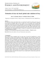
Fig. 3.20. a Latitudinal dependence of the parameter f
s
as per Li et al. (1995) (solid line)
and the values obtained from the airborne observations (dashed and dotted lines). Squares
point to the values of f
s
in total shortwave spectrum, circles point to the wavelength 0.5 µm;
b Dependence of the parameter f
s
of cosine of the solar incident angle as per Imre et al. (1996)
(nomograph) and the values obtained from the airborne observation. Squares indicate the
total spectrum data; triangles indicate the data at the wavelength 0.5
µm
120 Spectral Measurements of Solar Irradiance and Radiance in Clear and Cloudy Atmospheres
the study by Li et al. (1995). The results of this study include the latitudinal
dependence of parameter f
s

citedinFig.3.20aasasolidline.Theresultsofthe
airborne observations (Kondratyev 1972; Kondratyev et al. 1973a; Kondratyev
and Ter-Markaryants 1976; Kondratyev and Binenko 1981; Kondratyev and
Binenko 1984; Vasilyev O et al. 1987; Grishechkin et al. 1989; Vasilyev A et al.
1994) are presented in the same figure. Squares and dashed lines correspond to
the total shortwav e observations with the pyranometer , which almost coincide
with the data of the study by Li et al. (1995). Circles and dotted lines correspond
to the observations at a wav elength equal to 0.5
µm and they show crucially
larger values than the results of the total observations while keeping the same
latitudinal dependence. As hereinbefore described the values of parameter f
s
exceeding 2.0 indicate the high content of the absorbing aerosols together with
the large optical thickness of the cloud.
The variations of the anomalous absorption with solar zenith angle were
studied in Imre et al. (1996) and Minnet (1999). The authors Imre et al. (1996)
derived the relationship between parameter f
s
and solar zenith angle, which we
are citing in Fig. 3.20b (nomograph) together with our results of the airborne
observations (Kondratyev 1972; Kondratyev et al. 1973a; Kondratyev and Ter-
Markaryants 1976; Kondratyev and Binenko 1981, 1984; Vasilyev O et al. 1987;
Grishechkin et al. 1989; Vasilyev A et al. 1994) (squares indicate to tal spectrum
data, triangles indicate data at wavelength 0.5
µm). The solar angle dependence
of the airborne data of the total irradiances is evidently coinciding with the
data of Imre et al. (1996) while the dependence in question for wavelength
0.5
µm is significantly higher. It should be pointed out that the mentioned
coincidence reflects the essence of the specific features of radiation absorption

in cloudy atmosphere, though the results either by Imre et al. (1996) and Li et
al. (1995) or by Kondratyev (1972), Kondratyev et al. (1973a), Kondratyev and
Ter-Markaryants (1976), Kondratyev and Binenko (1981, 1984), Vasilyev O et al.
(1987), Grishechkin et al. (1989), and Vasilyev A et al. (1994) were obtained with
different instruments, methodologies of measurements and processing. Thus,
the excessive (anomalous) absorption really exists and it is mostly evinced in
the shortwave spectral region.
The main result of the study by Minnet (1999) is the following: “solar zenith
angle is critical in determining whether clouds heat or cool the surface. For
largezenithangles(
µ
0
> 0.15) the infrared heating of clouds is greater than
the reduction in insolation caused by clouds, and the surface is heated by the
presence of cloud. For smaller zenith angles, cloud cover cools the surface
and for intermediate angles, the surface radiation budget is insensitive to the
presence of or changes in, cloud cover.” The linear dependence of the cloud
radiative forcing upon the cosine of the solar zenith angle in the Arctic has
been revealed in the study by Minnet (1999).
The impact of the thick cloudiness and black carbon aerosols on the solar
radiation absorption has been revealed in the study by Liao and Seinfield
(1998) to produce the forcing values three times higher than those under the
cloud-free conditions. Moreover, it is increasing with the growth of cosine of
the solar zenith angle. Thus, the absorbing aerosols within the clouds cause
the cloud radiation absorption.
The Problem of Excessive Absorption of Solar Short-Wave Radiation in Clouds 121
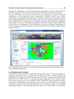
Fig. 3.21. The annual zonal cloud amount: (1) averaged over the latitude; (2) above the sea
surface and (3) above the ground surface in 1971–1990 according to Matveev et al. (1986)
The common features of the considered relationship are clear because of
the evident relation between the solar zenith angle and geographical latitude

(keeping in mind that the radiative experiments are accomplished around
midday). However, the original reaso n is not clear: whether it is the solar
height or different cloud optical properties in different latitudinal zones.
It is obvious that for elucidation of the cloud absorption a sufficient amount
of clouds is necessary. It is of special interest that the comparison of the
latitudinal dependence of the cloud amount (Fig. 3.21) from the study by
Matveev et al. (1986) and the dependence of parameter f
s
characterizing the
cloud radiative forcing as per Fig. 3.20b are seen to coincide qualitatively.
The airborne radiative experiments accomplished in the range of CAENEX,
GAAREX, GARP and GATE programs have apparently demonstrated a signif-
ican t absorption of SWR by clouds. In the remainder of this subsection the
following thesis are given:
The excessive absorption of SWR is defined just by the optical properties of
cloudiness and is not caused by the observational or processing uncertainties
as some investigators have presented.
1. The relationship between the scattering and absorbing properties of
stratus clouds and the geographical latitude, solar zenith angle, and type
of the atmospheric aerosols within clouds is experimentally proved.
2. The increase in radiation absorption is stronger in thick cloud layers in
a dusty atmosphere containing carbon or sand aerosols.
The effect of the excessive absorption is observed over the shortwave spectral
regionasawholebutitisespeciallyhighfortheshorterwavelengths(
λ < 0.7 µ).
The existence of the anomalous absorption fundamentally changes the current
understanding of the energetic budget of the atmosphere. In this connection,
it is of great importance to account for the atmospheric heating caused by the
cloudabsorptionofSWRforclimateforecastsimulations.
122 Spectral Measurements of Solar Irradiance and Radiance in Clear and Cloudy Atmospheres

3.6
Ground and Satellite Solar Radiance Observation in an Overcast Sky
This section presents brief information about the experiments whose results
have been used for the retrieval of the cloud optical parameters. There are
ground observations with thespectral instruments described invarious studies
(Mikhailov and Voitov 1969; Kondratyev and Binenko 1981; Radionov et al.
1981; Gorodetskiy et al. 1995; Melnikova et al. 1997) and satellite observations
with the POLDER instrument on board the ADEOS satellite (Deschamps et al.
1994; Breon et al. 1998).
3.6.1
Ground Observations
Thegroundobservationshaveincludedthetransmittedspectralradiancemea-
surements for several viewing angles. The conditions of their accomplishment
arelistedinTable3.3(thenumerationinthetablecontinuesTable3.2).The
first experiment was performed under overcast conditions at the drifting Arc-
tic station SP-22 on the 13th August and on the 8th October 1979 (Radionov
et al. 1981). The measurements had been carried out in the spectral interval
0.35–0.96
µm with resolution 0.001 µm, but the results were processed only at
11 spectral points in each spectrum. The error of the transmitted radiance mea-
surements was evaluated within 3% (Mikhailov and Voitov 1969; Radionov et
al. 1981). There were extended, horizontally homogeneous thick clouds during
the experiment.
The second exper iment was accomplished under the overcast condition in
St. Petersburg’s suburb on 12th April 1996 (Melnikova et al. 1997) with the
spectral instrument, constructed by the authors of the study by Gorodetskiy
et al. (1995) on the basis of the CCD matrix detector and with spectral res-
olution 0.002
µm and s pectral range 0.35–0.76 µm (Gorodetskiy et al. 1995).
Use of this spectrometer allowed registration of the signal within the spectral

ranges 0.35–0.76
µm simultaneously in every spectral point. The instrument
was characterized with small size and was PC or Notebook compatible thus,
it was convenient for field observations, provided the diminishing of some
observational uncertainties and allowed the initial data processing at once.
Tabl e 3 .3 . Details of the ground radiative experiments
No. Experiment µ
0
ϕ,
◦
NDate A
s
Other conditions
11 Arctic drifting
station SP-22
0.500 85 13 August 1979 0.60 Surface is wet snow
12 Arctic drifting
station SP-22
0.275 85 08 October 1979 0.90 Surface is fresh snow
13 Petrodvorets 0.620 60 12 April 1996 0.70 Surface is fresh snow
Ground and Satellite Solar Radiance Observation in an Overcast Sky 123
In all these cases, the data were obtained for 5 viewing angles (0
◦
,10
◦
,15
◦
,
45
◦

,70
◦
) and for 5 azimuth angles to control the cloudiness homogeneity. One
set of measurements took about 10 minutes in the Arctic experiments. The
measurements were accomplished at midday, when the solar zenith angle was
changing weakly during the 10-minute period. The transmitted radiance for
different azimuth angles and for the one viewing angle varying in the range of
the measurement error was averaged in the data processing.
During the Arctic experiment the observations of the downwelling and
upwelling irradiance were accomplished and ground albedo A was obtained
in Radionov et al. (1981). Different types of snow cover were studied (fresh
snow, wet snow and so on), and i n all cases the spectral dependence of ground
albedo A was weak. On the 13th August 1979, the ground surface was covered
with wet snow and ground albedo A was about 0.6. On the 8th October 1979,
the ground surface was covered with fresh snow and ground albedo A was
about 0.9.
In addition, the observation of direct solar radiation was carried out in
the clear sky during the Arctic experiment of 1979. It gave the opportunity of
calibrating the instrument in units of solar incident flux
πS at the top of the
atmosphere necessary for the retrieval of optical thickness
τ. The experiment
on 12th April 1996 was accomplished in a similar manner excluding the mea-
surement of direct solar radiation in the clear sky, hence the instrument was
not calibrated and optical thickness
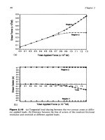
τ could not have been obtained. Figure 3.22
illustrates the spectral irradiances for cosines 1.0, 0.985, 0.966, 0.707, 0.340.
Fig. 3.22. Results of the transmitted radiance observation (relative units) for overcast sky on
12th April 1996
124 Spectral Measurements of Solar Irradiance and Radiance in Clear and Cloudy Atmospheres

3.6.2
Satellite Observations
The POLDER radiometer consisted of three principal components: a CCD
matrix detector, a rotating wheel carrying the polarizers and spectral filters,
and wide field of view (FOV) telecentric optics as described in Deschamps et
al. (1994). The optics had a focal length of 3.57 mm with a maximum FOV
of 114
◦
. POLDER acquired measurements in nine bands, three of which were
polarized.
All POLDER measurements were sent to Centre National des Etudes Spa-
tiales (CNES, France) where they were processed. One can find a detailed
description in Breon et al. (1998). Processed data have 3 levels of products.
Level-1 product consists of radiometric and geometric processing. It yields
top-of-the-atmosphere geocoded radiances. Level-2 processing generates geo-
physical parameters from individual Level-1 products, which cover the fraction
oftheEarthobservedduringoneADEOSorbitwithadequateilluminationcon-
ditions. POLDER Level-2 product is taken here for interpreting.
Tabl e 3 .4 . Details of the satellite experiments
No. Experiment, µ
0
ϕ,
◦
NDate Imageτ
0
ω
0
geographic site size
(pixels)
14 The Southwest 0.7–0.9 43.7–47.8 24 June 1997 388 15 0.996

part of Europe,
1.65
◦
E–32.04
◦
E
15 The Atlantic Ocean, and 0.7–0.9 43.7–47.8 24 June 1997 316 15 0.997
the South of France
24.80
◦
W–3.24
◦
E
16 The North Sea and the 0.6– 0.8 57.7–60.8 24 June 1997 316 20 0.995
West part of Scandinavia
−0.48
◦
E–17.22
◦
E
17 Scandinavia 0.6–0.8 57.7–60.8 24 June 1997 289 15 0.995
and the Baltic Sea
1.57
◦
–38.88
◦
E
18 Baltic Sea 0.6–0.8 57.7–60.8 24 June 1997 316 7 0.995
and the Northwest part
of Russia 27.65

◦
–66.72
◦
E
19 Southeast Asia 0.8–1.0 6.7–13.8 24 June 1997 585 40 0.995
and the Pacific Ocean
121.63
◦
–123.61
◦
W
20 The East part of Siberia, 0.7–0.9 45.7–51.3 24 June 1997 585 30 0.997
the Pacific Ocean, Sakhalin
Island 127.60
◦
–148.68
◦
W
References 125
The geometry for pixel was the following: the point remained within the
POLDER field while the satellite passed over it. As the satellite passed over
a target, from 6 up to 14 directional radiance measurements (for eac h spec-
tral band) were performed aiming at the point. Therefore, POLDER succes-
sive observations allowed the measurement of the multidirectional reflectance
properties of any target within the instrument swath.
Three wavelength channels with the centers at 443, 670 and 865 nm were
available for our analysis. The radiance multidirectional data were given in
units of the normalized radiance, i.e. the maximum spectral radiance divided
by the solar spectral irradiance at nadir and multiplied by
πµ

0
,whereµ
0
was
the cosine of the solar incident angle. The solar angle, azimuth angle, viewing
directions and cloud amount were also included to the data array. The date
of the observations under interpretation was 24 June 1997. Seven sites with
extended cloud fields were chosen.
The information about the satellite images used for the optical parameters
retrieval hereinafter are shown in Table 3.4. The values of the single scattering
albedo and the optical thickness typical for most of the pixels of the image are
presented in columns number eight and nine of the table. We should mention
that images 14 and 15 demonstrate the same cloud field, as do images 16–18.
References
Ackerman SA, Cox SK (1981) Aircraft observations of the shortwave fractional absorption
of non-homogeneous clouds. J Appl Meteor 20:1510–1515
Ackerman SA, Stephens GL (1987) The absorption of solar radiation by cloud droplets: an
application of anomalous diffraction theory. J Atmos Sci 44:1574–1588
Anderson TW (1971) The Statistical Analysis of time series. Wiley, New York
Arking A (1996) Absorption of solar energy in the atmosphere: Discrepancy between
a model and observations. Science 273:779–782
Berlyand ME, Kondratyev KYa, Vasilyev OB et al. (1974) Complex study of the specifics of
the meteorological regime of the big city, case study Zaporoghy e city (CAENEX-72).
Meteorology and Hydrology (1):14–23 (in Russian)
Bott A (1997) A numerical model of cloud-topped planetary boundary layer: Impact of
aerosol particles on the radiativeforcingof stratiform clouds.QJRMeteorolSoc 123:631–
656
Bréon F-M, CNES Project Team (1998) POLDER Level-2 Product Data Format and User
Manual. PA.MA.O.1361.CEA Edn. 2 – Rev. 2, January 26th
Cess RD, Zhang MH (1996) How much solar radiation do clouds absorb? Response. Science

271:1133–1134
Cess RD, Zhang MH, Minnis P, Corsetti L, Dutto n EG, Forgan BW, Garber DP, Gates WL,
Morcrette JJ, Potter GL, Ramanathan V, Subasilar B, Whitlock CH, Yound DF, Zhou
Y (1995) Absorption of solar radiation by clouds: Observation versus models. Science
267:496–499
Chapurskiy LI (1986) Reflection properties of natural objects within spectral ranges 400–
2,500 nm. Part I. USSR Defense Ministry Press (in Russian)
Chapurskiy LI, Chernenko AP (1975) Spectral radiative fluxes and inflows in the clear atmo-
sphere above the sea surface within the ranges 0.4–2.5
µ. Main Geophysical Observatory
Studies 366, pp 23–35 (in Russian)
126 References
Chapurskiy LI, Chernenko AP, Andreeva NI (1975) Spectral radiative characteristics of
the atmosphere during the sand storm. Main Geophysical Observatory Studies 366, pp
77–84 (in Russian)
Charlock TP, Alberta TL, Whitlock CH (1995) GEWEX data sets for assessing the budget for
the absorption of solar energy by the atmosphere. GEWEX News WC RP 5:9–11
Chou M-D, Arking A, Otterman J, Ridgway WL (1995) The effect of clouds on atmospheric
absorption of solar radiation. Geoph Res Lett 22:1885–1888
Collins W (1998) A global signature of enhanced shortwav e absorption by clouds. J Geophys
Res 103:31669–31679
Crisp D, Zuffada C (1997) Enhanced water vapor absorption within tropospheric clouds:
a partial explanation for anomalous absorption. In: IRS’96 Current Problems in At-
mospheric Radiation. Proceedings of the International Radiation Symposium, August
1996, Fairbanks, Alaska, USA. A. Deepak Publishing, pp 121–124
Danishevskiy YuD (1957) Actinometric instruments and methods of observations. Hydrom-
eteorologic Press, Leningrad (in Russian)
Deschamps PY, Bréon FM, Leroy M, Podaire A, Bricaud A, Buriez JC, Sèze G (1994) The
POLDER Mission: In strument Characteristics and Scientific Objectives. IEEE Trans
Geosc Rem Sens 32:598–615

Duran SB, Odell PL (1974) Cluster Analysis. A Survey. Springer, Berlin Heidelberg New York
Ermakov SM, Mikhailov GA (1976) Course of statistical modeling. Nauka, Moscow (in
Russian)
Evans WFJ, Puckrin E (1996) Near-infrared spectral measurements of liquid water absorp-
tion by clouds. Geophys Res Lett 23:1941–1944
Francis PN, Taylor JP,Hignett P,SlingoA (1997) Measurements from the U.K. Meteo rological
office C-130 aircraft relating to the question of enhanced absorption of solar radiation
by clouds. In: IRS’96 Current problems in Atmospheric Radiation. Proceedings of the
International Radiation Symposium, August 1996, Fairbanks, Alaska, USA. A. Deepak
Publishing, pp 117–120
Gorelik AL, Skripkin VA (1989) Methods of recognizing. High School, Moscow (in Russian)
Gorodetskiy VV, Maleshin MN, Petro v SYa, Sokolo va EA, Pchelkin VI, Solovyev SP
(1995) Small dimension multi-channel optical spectrometers. Optical J 7:3–9 (in
Russian)
Grishechkin VS, Melnikova IN (1989) Investigations of radiative flux divergence in stratus
clouds in Arctic. In: Rational Using of N atural Resources. Polytechnic University Press,
Leningrad, pp 60–67 (in Russian)
Grishechkin VS, Melnikova IN, Shults EO (1989) Analysis of spectral radiative character-
istics. LGU, Atmospheric Physics Problems 20. Leningrad University Press, Leningrad,
pp 20–30 (in Russian)
Harshvardhan, Ridgway W, Ramaswamy V, Freidenreich SM, Batey MJ (1998) Spectral
characteristics of solar near-infrared absorption in cloudy atmospheres. J Geophys Res
103(D22):28793–28799
Hayasaka T, Kikuchi N, Tanaka M (1994) Absorption of solar radiation by stratocu-
mulus clouds: aircraft measurements and theoretical calculations. J Appl Meteor
1047–1055
Hegg D (1986) Comments on “The effect of very large drops on cloud absorption. Part I:
Parcel models.” J Atmos Sci 43:399–400
Hignett P, Taylor JP (1996) The radiative properties of inhomogeneous boundary layer
cloud: Observations and modelling. QJR Meteorol Soc 122:1341–1364

Hobbs V (ed) (1993) Aerosol-Cloud-Climate Interaction. Academic Press, New York
References 127
Imre DG, Abramson EN, Daum PH (1996) Quantifying cloud-induced short-wa ve absorp-
tion: an examination of uncertainties and recent arguments for large excessive absorp-
tion. J Appl Met 35:1191–2010
Ivlev LS, Popova CI (1975) Optical constants of atmospheric aerosols substance. Izv. USSR
High Schools, Physics 5:91–97 (in Russian)
Ivlev LS, Andreev SD (1986) Optical properties of atmospheric aerosols. Leningrad Univer-
sity Press, Leningrad (in Russian)
Kalinkin NN (1978) Numerical methods. Nauka, Moscow (in Russian)
Kiehl JT et al. (1995) Sensitivity of a GCM climate to enhanced shortwave cloud absorption.
J Climate 8:2200–2212
King M D, Si-Chee Tsay, Platnick S (1995) In situ observations of the indirect effects of
aerosols on clouds. In: Charlson RJ, Heitzenberg J (eds) Aerosol forcing of climate.
Wiley, New York
Kolmogorov AN, Fomin SV (1999) Elements of the theory functions and the functional
analysis. Dover Publications
Kondratyev KYa (1972) Complex Atmospheric Energetic Experiment. GARP Publ. Series.
WMO, Geneva (12)
Ko ndratyev KYa, Ter-Markaryants NE (eds) (1976) Complex radiation experiment. Gydr o-
meteoizdat, Leningrad (in Russian)
KondratyevKYa, BinenkoVI (eds)(1981)First global experimentFGGE, vol2. Polar aerosols,
extended cloudiness and radiation. Gy drometeoizdat, Leningrad, pp 89–91 (in Russian)
Kondratyev KYa, Binenko VI (1984) Impact of Clouds on Radiation and Climate. Gydro-
meteoizdat, Leningrad (in Russian)
Kondratyev KYa, Vasilyev OB, Grishechkin V S et al. (1972) Spectral shortwave radiative flux
divergence in the tropos phere. Doklady RAS, Iss Math Phys 207:334–336 (in Russian)
Kondratyev KYa, Vasilyev OB, Grishechkin VS et al. (1973a) Spectral radiative flux di-
vergence of radiation energy in the troposphere within the spectral ranges 0.4–2.4
µ.

I. Methodology of observations and data processing. Main Geophysical Observatory
Studies. 322:12–23 (in Russian)
Kondratyev KYa, Vasilyev OB, Ivlev LS et al. (1973b) The aerosol influence on radiation
transfer: possible climatic consequences. Leningrad University Press, Leningrad (in
Russian)
Kondratyev KYa, Vasilyev OB, Grishechkin V S et al. (1974) Spectral shortwave radiative flux
divergence in the troposphere and their variability. Izv. RAS, Atmosphere and Ocean
Physics 10:453–503
Kondratyev KYa, Vasilyev OB, Ivlev LS et al. (1975) Complex observational studies above
the Caspian Sea (CAENEX-73). Meteorol H ydrol 7:3–10 (in Russian)
Ko ndratyev KYa, Lominadse VP, Vasilyev OB et al. (1976) Complex study of radiation
and meteorological regime of Rustavi city. (CAENEX-72). Meteor ol Hydrol 3:3–14 (in
Russian)
Kondratyev KYa, Binenko VI, Vasilyev OB, Grishechkin VS (1977) Spectral radiative char-
acteristics of stratus clouds according CAENEX and GATE data. Proceedings of Sym-
posium Radiation in Atmosphere, Garmisch-Partenkirchen 1976, Science Press, pp
572–577
Kondratyev KYa, Vasilyev OB, Fedchenko VP (1978) The attempt of the soils detection by
their reflection spectra. Soil Sci 4:5–17 (in Russian)
Kondratyev KYa, Korotkevitch OE, Vasilyev OB et al. (1987) Color characteristics of Ladoga
Lake waters. In: Complex remote lakes monitoring. Nauka, Leningrad, pp 55–60 (in
Russian)
128 References
Kondratyev KYa, Vlasov VP, Vasilyev OB et al. (1987) Spectral optical characteristics of
the melting snow cover (case studies the Onega Lake and the White Sea). In: Complex
remote lakes monitoring. Nauka, Leningrad, pp 211–217 (in Russian)
Kondratyev KYa, Pozdnyakov DV, Isakov VYu (1990) Radiation – hydrooptics experiments
in lakes. Nauka, Leningrad (in Russian)
Kondratyev KYa, Binenko VI, Melnikova IN (1996) Cloudiness absorption of solar radiation
in visual spectral region. Meteorology and Hydrology 2:14–23 (in Russian)

Kondratyev KYa, Binenko VI, Melnikova IN (1997a) Absorption of solar radiation by clouds
and aerosols in the visible wavelength region at different geog raphic zones. CAS/WMO
working group on numerical experimentation, WMO, Geneva
Kondratyev KYa, Binenko VI, Melnikova IN (1997b) Absorption of solar radiation by clouds
and aerosols in the visible wavelength region. Meteorology and Atmospheric Physics
(0/319):1–10
Li Zhanging, Howard WB, Moreau L (1995) The variable effect of clouds on atmospheric
absorption of solar radiation. Nature 376:486–490
Liao H, Seinfield JH (1998) Effect of clouds on direct aerosol radiative forcing of climate. J
Geoph Res 103(D4):3781–3788
LubinD,Chen J-P, Pilewskie P,RamanathanV, ValeroPJ(1996)Microphysicalexaminationof
excessive cloud absorption in the tropical atmosphere. J Geophys Res 101(D12):16,961–
16,972
Makarova EA, Kharitonov AV, Kazachevskaya TV (1991) Solar irradiance. Nauka, Moscow
(in Russian)
Mars hak A, Davis A, Wiscombe W, Cahalan R (1995) Radiative smoothing in fractal clouds.
J Geophys Res 100(D18):26247–26261
Matveev LT, Matveev YuL, Soldatenkov SA (1986) Global field of cloudiness. Gydrometeoiz-
dat, Leningrad (in Russian)
Melnikova IN, Domnin PI, Varotsos C, Pivovarov SS (1997) Retrieval of optical properties of
cloud layers from transmitted solar radiance data. Proceeding of SPIE, vol. 3237, 23-d
European Meeting on Atmospheric Studies by Optical Methods, September 1996, Kiev,
Ukraine, pp 77–80
Mikhailov VV, Voytov VP (1969) An improved model of universal spectrometer for inves-
tigation of short-wav e radiation field in the atmosphere. In: Pr oblems o f Atmospheric
Physics. 6:Leningrad University Press, Leningrad, pp 175–181 (in Russian)
Minin IN (1988) The theory of radiation transfer in the planets atmospheres. Nauka, Moscow
(in Russian)
Minnet P (1999) The influence of solar zenith angle and cloud type on cloud radiative
for cing at the surface in the Arctic. J Climate 12:147–158

Molchanov NI ( ed) (1970) Set of computer codes of small electronic-digital computer “Mir”.
vol 1. Methods of calculations. Naukova dumka, Kiev (in Russian)
Monin AC (1982) Introduction to theory of climate. Gydrometeoizdat. Leningrad (in Rus-
sian)
Mulamaa YuAR (1964) Atlas of optical characteristics of waving sea surface. Estonian AS
Press, Tartu (in Russian)
Nesmelova LI, Rodimova OB, Tvorogov SD (1997) Absorption by water vapor in the near
infrared region and certain geophysical consequences. Atmosphere and Ocean Optics
10:131–135 (Bilingual)
O’Hirok, Gautier C (1997) Modelling enhanced atmospheric absorption by clouds. IRS’96.
Current problems in Atmospheric Radiation. Proceedings of the International Ra-
diation Sym posium, August 1996, Fairbanks, Alaska, USA. A. Deepak Publishing,
References 129
pp 132–134
Otnes RK, Enochson L (1978) Applied Time-Series Analysis. Toronto. Wiley, New York
Pilewskie P, Valero FPJ (1995) Direct observations of excessive solar absorption by clouds.
Science 267:1626–1629
Pilewskie P, Valero FPJ (1996) Ho w much solar radiation do clouds absorb? Respo nse.
Science 271:1134–1136
Poetzsch-Heffter C, Liu Q, Ruprecht E, Simmer C (1995) Effect of cloud types on the Earth
radiation budget calculation with the ISCCP C1 da taset: Methodology and initial results.
J Climate 8:829–843
Radionov VF, Sakunov GG, Grishechkin VS (1981) Spectral albedo of snow surface from
measurements at drifting station SP-22. In: Kondratyev KYa, Binenko VI (eds) First
global experiment FGGE, vol 2. Polar aerosols, extended cloudiness and radiation.
Gidrom eteoizdat, Leningrad, pp 89–91 (in Russian)
Ramanathan V, Subasilar B, Zhang GJ, Conant W, Cess RD, Kiehl JT, Grassl G, Shi L (1995)
Warm Pool Heat Budget and Shortwave Cloud Forcing: a Missing Physics?. Science
267:500–503
Ramanathan V, Vogelman AM (1997) Greenhouse effect, atmospheric solar absorption and

the Earth’s radiation budget: From the Arrhenius–Langley era to the 1990s. Ambio
26:38–46
Ramaswamy V,Freidenreich SM (1998) A high-spectral resolution study of the near-infrared
solar flux disposition in clear and overcastatmospheres. J Geophys Res 103(D18):23,255–
23,273
Romanova LM (1992) Space varia tion of radiative characteristics of horizontally inhomo-
geneous clouds. Izv RAS Atmosphere and Ocean Physics 28:268–276 (Bilingual)
Savijärvi H, Arola A, Räisänen P (1997) Short-wave optical properties of precipita ting water
clouds. QJR Meteorol Soc 123:883–899
Shettle EP (1996) The data were tabulated in Naval Research Laboratory and were used to
generated the aerosol models which are incorporated into the LOWTRAN, MODTRAN
and FASCODE computer codes. Data form HITRAN-96 cd-rom media
Skuratov SN, Vinnichenko NK, Krasnova TM (1999) Observations of upwelling and down-
welling solar shortwave irradiances with the stratospheric airplane “Geo physics” in the
Tropics (Seishel Islands, February-March 1999). In: International Symposium of for-
mer USSR “Atmospheric radiation (ISAR–99)”. St. Petersburg, NICHI, St Petersburg
University, pp 58–59 (in Russian)
Sobolev VV (1972) The light scattering in the planet atmospheres. Nauka. Moscow (in
Russian)
STANDARDS 4401–81. Standard atmosphere. USSR state standard (1981) Standard’s Press,
Moscow (in Russian)
Stephens G (1995) Anomalous shortwave absorption in clouds. GEWEX News, WCRP 5:5–6
StephensG(1996)Howmuch solar radiationdoclouds absorb? Technical comments. Science
271:1131–1133
Stephens G, Tsay SC (1990) On the cloud absorption anomaly. Quart J Roy Meteorol Soc
116:671–704
Taylor JP, Edwards JM, Glew MD, Hignett P, Slingo A (1996) Studies with a flexible new
radiation code. II. Comparison with aircraft short-wave observations. QJR Meteorol
Soc 122:839–861
Tito v GA (1988) Mathematic modeling of radiative characteristics of broken cloudiness.

Atmosphere and Ocean Optics 1:3–18 (Bilingual)
Ti tov GA (1996) Radiation effects of inhomogeneous stratus-cumulus clouds: Horizontal
130 References
transport. Atmosphere and Ocean Optics 9:1295–1307 (Bilingual)
Titov GA (1996) Radiation effects of inhomogeneous stratus-cumulus clouds: Absorption.
Atmosphere and Ocean Optics 9(10):1308–1318 (Bilingual)
Titov GA, Ghuravleva TB (1995) Spectral and total absorption of solar radiation within
broken cloudiness. Atmospheric and Ocean Optics 8:1419–1427
Titov GA, Zhuravleva TB (1995) Absorption of solar radiation in broken clouds. Proceedings
of the Fifth ARM Science Team Meeting, San Diego, California, USA, 19–23 March, pp
397–340
Titov GA, Kasyanov EI (1997) Radiation properties of inhomogeneous stratus-cumulus
clouds with the stochastic geometry of the top boundary. Atmosphere and Ocean Optics
10:843–855 (Bilingual)
Valero FPJ, Cess RD, Zhang M, Pope SK, Bucholtz A, Bush B, Vitko J,Jr (1997) Absorp-
tion of solar radiation by the cloudy atmosphere: interpretations of collocated aircraft
measurements. J Geophys Res 102(D25):29,917–29,927
Vasilyev AV, Ivlev LS (1997) Empirical models and optical characteristics of aerosol en-
sembles of two-layer spherical particles. Atmosphere and Ocean Optics 10:856–868
(Bilingual)
Vasilyev AV, Melnikova IN, Mikhailov VV (1994) Vertical profile of spectral fluxes of scat-
tered solar radiation within stratus clouds from airborne measurements. Izv. RAS,
Atmosphere and Ocean Physics 30:630–635 (Bilingual)
Vasilyev AV, Melnikova IN, Poberovskaya LN, Tovstenko IA (1997a) Spectral brightness
coefficients of natural ground surfaces in spectral ranges 0.35–0.85
µ on base of airborne
measurements. I. Instruments and processing methodology. Earth Observations and
Remote Sensing 3:25–31 (Bilingual)
Vasilyev AV, Melnikova IN, Poberovskaya LN, Tovstenko IA (1997b) Spectral brightness
coefficients of natural ground surfaces in spectral ranges 0.35–0.85

µ on base of air-
borne measurements.II. Water surface. Earth Observations and RemoteSensing4:43–51
(Bilingual)
Vasilyev AV, Melnikova IN, Poberovskaya LN, Tovstenko IA (1997c) Spectral brightness
coefficients of natural ground surfaces in spectral ranges 0.35–0.85
µ on base of airborne
measurements. III. Ground surface. Earth Observations and Remote Sensing 5:25–32
(Bilingual)
Vasilyev OB (1986) To the methodology of spectral brightness coefficients and spectral
albedo of natural objects. In: Zanadvorov PN (ed) Possibility of studies of natural
resources with remote methods. Leningrad University Press, Leningrad, pp 95–105 (in
Russian)
Vasilyev OB, Grishechkin VS, Kashin FV et al. (1982) Studies of the spectral transmissivity of
the atmosphere, spectral phase functions and determination of the aerosol parameters.
In: Atmospheric physics problems. Iss 17, Leningrad University Press, Leningrad, pp
230–246 (in Russian)
Vasilyev OB, Grishechkin VS, Kondratyev KYa (1987) Spectral radiative characteristics of
thefreeatmosphereabovetheLadogaLake.In:Complexremotelakesmonitoring.
Nauka, Leningrad, pp 187–207 (in Russian)
Vasilyev OB, Grishechkin VS, Kovalenko AP et al. (1987) Spectral information – measuring
systemfor airborne and ground study of the shortwave radiation field in the atmosphere.
In: Complex remote lakes monitoring. Na uka, Leningrad, pp 225–228 (in Russian)
Vasilyev OB, Contreras AL, Velazques AM et al. (1995) Spectral optical properties of the pol-
luted a tmosphere ofMexic oCity (spring–summer 1992). J GeophysRes 100(D12):26027–
26044
References 131
Wiscombe WJ (1995) An absorbing mystery. Nature 376:466–467
Wiscombe WJ, Welch RM, Hall WD (1984) The effect of very large drops oncloud absorption.
Part I:Parcel models. J Atmos Sci 41:1336–1355
Yamanouchi T, Charlock TP (1995) Comparison of radiation budget at the TOA and surface

in the Antarctic from ERBE and ground surface measurements. J Climate 8:3109–3120
Zhang MH, Lin WY, Kiehl JT (1998) Bias of atmospheric shortwave absorption in the
NCAR Community Climate Models 2 and 3:Com parison with monthly ERBE/GEBA
measurements. J Geophys Res 103:8919–8925
Zuev VE, Krekov GM (1986) Optical models of the atmosphere.(Recent problems of the
atmospheric optics, vol. 2). Gydrometeoizdat, L eningrad (in Russian)
CHAPTER 4
The Problem
of Retrieving Atmospheric Parameters
from Radiative Observations
This chapter presents a general statement of the problem of determination of
atmospheric and surface parameters from observational results of radiative
characteristics. The methods of determining the parameters of the radiative
transfer theoretical model providing the minimal standard deviation (SD)
between the numerical and measured results for the correspondent charac-
teristics are considered below in detail. The choice of a concrete set of the
parameters, the influence of systematic uncertainties of the numerical simu-
lations and the technical realization of the considered methods are discussed
further.
4.1
Direct and Inverse Problems of Atmospheric Optics
Hereinbefore described in Chaps. 1 and 2 we have demonstrated the possibil-
ities for solving the problem of calculating the solar radiance and irradiance
after setting the parameters of the atmosphere and gro und surface (volume
coefficients of absorption and scattering, phase function, and surface albedo).
Furthermore, the results of the characteristic radiative observations have been
presented in Chap. 3. Therefore, this gives us the possibility of relating the
problem of selecting the atmospheric parameters, which allowed computing
values to be equal to the measured characteristics. The problems considered in
Chap.2,i.e.calculationsoftheobservationalcharacteristicswiththechosen

parameters of the atmosphere and surface, are specified as direct problems
of atmospheric optics. Contrary to this, the problems considered below, i. e.
determination of the atmospheric and surface parameters from observational
results of the radiative characteristics, are specified as inverse problems of
atmospheric optics.
The solution of the direct problem implies the creation of the ma themat-
ical model of observations, on the basis of which one can relate the physical
notions concerning the interaction of radiation with atmosphere and surface
(see Chap. 1). We should point out two important obstacles for further consid-
eration.
Firstly, the choice of the physical and consequently mathematical models
of the mentioned processes is ambiguous. Actually, while creating the mathe-
matical descriptions, different idealizations of the concrete physical processes
134 The Problem of Retrieving Atmospheric Parameters from Radiative Observations
together with simplifications and approximations are inevitable, so any model
is simpler than the reality is, so it is inadequate when compared to the reality
to a certain degree. Hence, the choice of the concrete model together with its
parameters i s always ambiguous and it is defined either with the physical pro-
cesses put to the model, or with the degree of approximation of the description
of these processes. For example, if we are considering only the radiative trans-
fer, the parameters of the model will be the following: optical thickness, single
scattering albedo, and phase function (see Sect. 1.3). Then we could account
for the processes of the radiation-media int eraction defining the mentioned
values (see Sect. 1.2), and the parameters of the model will be: vertical profiles
of the pressure, temperature, concentrations of the atmospheric gases, and
volume coefficients of the aerosol scattering and absorption.
Secondly, the number of parameters describing the mentioned processes
is always fini te in the rang e of the chosen model.Itisreadilyseenfromthe
technical point of view and needs no comment. However, from the other side
the number of the measured characteristics is finite too. Actually, if even the

contin uous spectrum of the irradiance or radiance is registered, really it is
representing as a finite array of the measured characteristics (see Sect. 3.1).
The opposite case is impossible because of digitations of the output signal.
Thus,itissafetosaywithoutthegeneralitylossthatwhilesolvingthedirect
problem we realize an algorithm allowing the calculation of a strictly limited
set of values through a strictly limited set of parameters. This statement is
expressed with the mathematically formal relation:
˜
Y
= G(U), (4.1)
where
˜
Y ≡ (˜y
i
), i = 1, ,N is the set, i.e. the vector, of the calculated val-
ues, corresponding to real N measurements; G is the operator of the direct
problem solving, i. e. the realization of a certain (concretely chosen as has
been pointed out above) mathematical model of the observational process;
U
= (u
j
), j = 1, ,M is the vector of parameters of the model in question.
In general the components of vectors
˜
Y and U could be inhomogeneous, i. e.
could have different meaning and different units (it is always so for vector U).
We should m e ntion that vector U includes all necessary parameters for solving
the direct problem (not only parameters characterizing the atmosphere and
surface but also the solar zenith angle, value of the incident flux at the top of the
atmosphere, spectroscopic parameters for computing the volume coefficient

of the molecular absorption – Sect. 1.2 etc.), and vector
˜
Y contains only the
observa tional r esults.
The formal statement of the inverse problem is determination (in atmo-
spheric optics it is accepted to say retrieval)ofthecomponentsofparameter
vector U with the specified concrete values of observational result vector Y.
However, there is no sense in retrieving all parameters included in vector U.
Actually, some parameters of vector U, for example the solar zenith angle, are
known (exacter: are supposed to be known). Therefore, from the components
of vector U let us select vector X ≡ (x
k
), k = 1 ,K, which has to be retrieved.
The concrete variants of this selection are considered in the study by Timofeyev
Direct and Inverse Problems of Atmospheric Optics 135
(1998) where it is proposed to classify the inverse problems coming from the
type of known and desired parameters. We will return to the topic of choice
in Sect. 4.3, and now let us assume that the concrete parameters contained in
vector X are specified. Equation (4.1) could now be rewritten as:
˜
Y(X)
= G(X, U \X), (4.2)
where U \ X is the set of vector U components not included in vector X,i.e.
the known parameters of the direct problem. Thus: G(U)
= G(X, U \ X), i.e.
solution of the direct problem is not to depend on which parameters are to be
retrieved.
The inverse problem could be formulated as a determination of vector X
from the equation:
G(X, U \ X)

= Y . (4.3)
However, in a general case system (4.3) may have no solution. Indeed, as has
been shown above, the operator of the direct problem G is just an appro xi-
mation of reality. Hence, even if we supposed that it reflected reality exactly,
vector Y wouldnotbeadequatetorealitybecauseofthesystematicandran-
dom observational uncertainties. Thus, a set of possible solutions of the direct
problem
˜
Y(X) could disagree with a set of possible values of the observational
results Y. In addition, the case of the nonexistence of the solution for (4.3) is
quite a likely one, even in the simplest variant of the linear operator G.Itiscon-
nected with the general properties of the abstract linear operators (Tikhonov
and Aresnin 1986; Kolmogorov and Fomin 1989). However in our version of
the inverse problem statement it is evident: if observations {y
i
} are linearly
independen t and their quantity exceeds the quantity of the parameters under
retrieval (M>K), the system of the linear equations will be unsolved. There-
fore, generally the inverse problem of atmospheric optics can be formulated
as follows: to find a set of parameters of the direct problem so that its solution
would be as close as possible to the observational results. In mathematical
wording given in the book by Tikhonov and Aresnin (1986), it means to find
value X, for which the minimum is reached:
min
X∈T
ρ(Y,
˜
Y(X)) = min
X∈T
ρ(Y, G(X, U \ X)) , (4.4)

where T is the set of possible solutions, ρ(. . .) is the certain measure in space
of the observational vector s, i.e. the metrics (more details are in the book by
Kolmogorov and Fomin 1989). Note that in particular cases the minimum in
question could be equal to zero, i.e. the equality in relation Y
= G(X, U \ X)is
possible.
The essential factor, which is to be accounted for while solving the inverse
problem, is the observational uncertainty. These questions will be considered
in further detail and here we only mention that unknown parameters X are
determined with the uncertainty as well. Hence, accounting for the unc ertainty
is an alienable and important stage of the inverse problem solving in atmo-
spheric optics. Besides, as the base of the inverse problem solving consists of
136 The Problem of Retrieving Atmospheric Parameters from Radiative Observations
thecomparisonbetweentheobservationalresultsandsolutionofthedirect
problem, the inverse problems are solved with the accuracy defined with the
uncertainty of the selected model parameters choice, i. e. with the concrete
choice of operator G. Hence, the stage of the choice of method for the direct
problem solving is the most important part of solving the inverse problem. Be-
sides, as has been mentioned above, the operator of the direct problem solving
is inevitably approximated in any case; hence, the account of the approxima tion
influence on the results is necessary as well.
In conclusion, the following general scheme for numerically solving the
inverse problems in atmospheric optics could be proposed:
1. Studying the contemporary theory of the physical processes forming the
measured characteristics.
2. Choosing a concrete mathematical model of the observations together
with its parameters, r ealization of this model on computer.
3. The erro r analysis of the direct problem.
4. Dividing the parameters of the mathematical model to the known ones
andtothesubjectsoftheretrieval.

5. Choosing the method for solving the inverse problem. Estimating its
accuracy.
6. Realization of the solving algorithm on computer.
7. Observational data processing, the analysis and interpretation.
Excluding the first one, which has been considered in Chap. 1 we will discuss
all listed stages further, applying them to concrete inverse problems. However,
the survey is more appropriate in a different order from that listed above. We
should mention that firstly the described scheme has been proposed acc ording
to the results of the accomplished observations, so the actual problem of the
optimal experimentplanning will notbe touched upon.Secondly, the presented
algorithm has a more complicated logic in practice; in particular, returning to
previous stages with the purpose of verifying the model and modernization of
the numerical methods are possible. Thus, the numerous consequent versions
of the processed results presented in the studies by Chu et al. (1989, 1993)
and Steele and Turko (1997) are the standard situation while processing the
observational data of atmospheric optics. In fact, it is well known to specialists:
the results of the field observations in majority is impossible to process once
and for all, there is always something to improve.
We will not review the huge volume and variety of recent inverse problems
of atmospheric optics and methods of their solution. As has been mentioned
hereinbefore a certain classification of these problems was presented in the
study by Timofeyev (1998), and concerning the solution methods there has
been no classification for them yet. Here we will confine ourselves only to
the concrete inverse pro blems of retrieval of the atmospheric and surface
parametersfromtheresultsoftheairborneandsatelliteobservationsofthe
solar spectral radiance and irradiance in the atmosphere considered in Chap. 3.
Direct and Inverse Problems of Atmospheric Optics 137
It is possible to distinguish two essentially different cases: clear and overcast
sky.
In case of the overcast sky, we succeeded in obtaining the explicit analytical

solution, i. e., to write the components of vector X through the results of
observations Y as explicit analytical exp ressions. Moreover, these expressions
are not the approximations or empirical formulas, which are often used, but
the consequences of the rigorous relations of the radiative transfer theory.
We should point out that deriving similar relations for the inverse problem
of atmospheric optics is a rather rare case against the backcloth of the recent
mass enthusiasm for the numerical solving of the inverse problems on PC.
Actually, it corresponds to the philosophical traditions of physics according
to which the analytical methods of description of the natural phenomena are
preferable.
As follows from the results of the well-known study by Tikhonov (1943)
concerning the mathematical aspects of the inverse problem theory: if the in-
verse problem solution is the limited set of continues functions
1
(the analytical
solution is the limited set), this solution will be stable. It has been shown in
the book by Prasolov (1995) that the analysis of the stability of the inverse
problem solution (robustness) in the limited class of functions is reduc ed to
the statement of the intervals of the continuity of the functions describing the
solution. It follows from Chebyshev theorems about the solution stability in
the polynomials basis and from the Weierstrass theorem about the existence
of the uniform limit (converging to the solution) in the con tinuous function
space. In the case of the analytical solution, its analysis for the continuity is not
complicated. Further, the corresponding results will be presented while in de-
tail considering the possibilities of the analytical approaches. The derivations
of the pointed analytical relations will be shown in Chap. 6, and the analysis of
the results of the observational data processing for the cloudy atmosphere will
be considered in Chap. 7.
Regretfully, a similar analytical solution for the clear atmosphere h as not
succeeded. It is easy to understand it basis on general principles. The variant of

the overcast sky, when only the diffused radiation is measured, and the variant
of the pure clear atmosphere, when only the direct radiation is accounted for
(the optical thickness is easily obtained from Beer’s law) are the limit cases of
very strong diffusion or its absence. The real clear atmosphere is an interme-
diate case from the point of view of the diffuse strength and the intermediate
cases are usually more complicated than the limit ones. So, while processing
theverticalprofilesofthespectralirradiances,(Chap.3)theinverseproblem
has been put as a problem of numerical choice of the parameters satisfying
theabove-formulateddemandoftheminimummin
X∈T
ρ(Y, G(X, U \X)). The
search for the minimum (4.4) is not physical but a mathematical problem.
Thus, in this chapter this solution will be considered from the mathematical
side while accounting for the physical conditions and observational errors.
1
IntheoriginalwordingbyAndreyTikhonov,theterm“continuesmappinginthecompactspace”
is used. It is more general than that which we are using but these terms coincide in the case of finite
dimensioned space, which we are considering.
138 The Problem of Retrieving Atmospheric Parameters from Radiative Observations
The solution of the inverse problem for the irradiance observations in the
atmosphere and its results will be described in Chap. 5.
Before we present the concrete formulas and algorithms of the search for
minimum (4.4), we will mark that the mathematical aspects of the mentioned
problem solving are presented often in a rather abstract manner (Kondratyev
and Timofeyev1970)(comingfrom the approaches of variationcalculus and the
theory of self conjugate operators in Gilbert space, Elsgolts 1969; Kolmogorov
and Fomin 1989). Sometimes it is com plicated in practical applications of
the abstract expressions and they are perceived as formal receipts for the
problem solving without the real physical meaning. Besides, the important
questions of the choice of the mathematical model for the direct problem

solving, the choice of its concrete parameters and their influence are out
of the scope of such a presentation. Our experience of solving the inverse
problems of atmospheric optics demonstrates that the understanding of the
physical meaning of the relations in use plays an important role together
with the formal mathematical approaches. Thus, we will try to present the
indicated mathematical approaches not from the abstract positions but from
the applied ones in the simplest manner not ignoring even the technical aspects
of the realization. To understand such a presentation knowledge of linear
algebra (Ilyin and Pozdnyak 1978) and mathematical statistics (Cramer 1946)
is enough. We should mention that it is very convenient for comprehension and
analysis of the described approaches to consider them applying to the p roblems
of the minimal dimensions (one-dimensional and two-dimensional).
The methodology presented below is not the only approach to the search for
minimum (4.4). In fact, the stated problem relates to the class of mathemat-
ical extreme problems, whose solutions are well known nowadays (Vasilyev
F 1988). For example, in practice such elementary manner as a sorting of
a limited quantity of the vector X variants (Kaufman and Tanre 1998) is often
used for the solution search. However, the methodology described below is the
mathematically faultless one and allows for the correct account of the obser-
vational uncertainties that is particularly important. Its application becomes
increasingly popular with the development of the possibilities of computer
techniques.
Wewillbeginthepresentationfromthedefinitionofthedistancebetween
the vectors. Let us use the standard Euclid metrics (Kolmogorov and Fomin
1989) i.e. assume the following:
ρ(Y
(1)
, Y
(2)
) =

1
N




N

i=1
(y
(1)
i
− y
(2)
i
)
2
. (4.5)
The matter of Euclid metrics (4.5) is the SD of two vectors, i.e. from the physical
point of view we are interested in the closeness between the observational
results and the direct problem solution in average over the entire observational
data set i
= 1, ,N. The choice of this metric is predetermined because only it
succeeds the construction of the real algorithms for the search of the metrics
minimum. For example, if we take not an average difference between the
The Least-Square Technique for Inverse Problem Solution 139
observational and calculation results but the one, maximum over all points
i
= 1, ,N, the path described below will become impassable.
The distance between the observational and calculated values of R ≡

ρ(Y, G(X, U \ X)) is called adiscrepancy. Thus, finally it is possible to de-
fine the formulated problem as the revealing of the values of the vector X
components through the known observational vector Y corresponding to the
minimum of discrepancy:
R
=
1
N




N

i=1
(y
i
− ˜y
i
)
2
,
˜
Y = G(X, U \ X). (4.6)
The problem formulated in this manner constitutes the matter of aleast-
squares technique (LST), proposed by CF Gauss. The following section contains
the consequent elucidating of the LST, its specifics and modification.
4.2
The Least-Square Technique for Inverse Problem Solution
Write the solution of the direct problem explicitly through the vector compo-

nents of the observations and initial parameters:
˜y
i
= g
i
(x
1
, ,x
K
), i = 1, ,N , (4.7)
where g
i
( )arecertainfunctionswherethecomponentsofvectorU \ X are
included, however we will not write them further in the explicit relations.
Substituting (4.7) to the expression for discrepancy (4.6) and considering the
square of discrepancy R
2
as a function of variables x
k
, k = 1, ,K to obtain its
extremums we derive the following equation system:
∂R
2
∂x
k
= 0,
i.e.thesameindetail:
N

i=1

(y
i
− g
i
(x
1
, ,x
K
))
∂g
i
(x
1
, ,x
K
)
∂x
k
= 0, k = 1, ,K . (4.8)
Inthecommoncaseofnonlinearfunctionsg
i
the direct obtaining of the
solutions of system (4.8) and their analysis for the minimum of discrepancy are
rather complicated. Thus, to begin with, consider the case of linear functions g
i
,
which could be further generalized to the nonlinear dependence. Besides the
problems of obtaining the parameters of the linear dependence with LST often
appear, f or example these very problemshave been solved during the secondary
processing of the airborne irradiance data (Sect. 3.2).

140 The Problem of Retrieving Atmospheric Parameters from Radiative Observations
Equation (4.7) in the case of the linear dependence is written as follows:
˜y
i
= g
i0
+
K

k=1
g
ik
x
k
. (4.9)
Coefficients g
i0
, g
ik
are not to be the identical constants at all. They can be
rather complicated functions o f vector U\X. It should only be noted that the
coefficientsare constants from the sense of the considered relationship between
the observations and desired parameters because all parameters of vector U\X
are known and fixed within the range of the concrete inverse problem. The
substitution of (4.9) to equation system (4.8) leads to the system of K linear
algebraic equations with K unknowns:
K

j=1
x

j

N

i=1
g
ij
g
ik

=
N

i=1
(y
i
− g
i0
)g
ik
, k = 1, ,K . (4.10)
Rewrite (4.10) in the matrix form using above-defined vectors X ≡ (x
k
),
Y ≡ (y
i
) and introducing vector G
0
≡ (g
i0

) together with matrix G ≡ (g
ik
),
i
= 1, ,N, k = 1, ,K:
(G
+
G)X = G
+
(Y − G
0
) (4.11)
where the sign “+” specifies the matrix transposition. The vectors are assumed
as columns; the first indices of the matrix are assumed as indices of a line while
writing system (4.11), and we will stick to this order. Multiplying both parts of
(4.11) from the left-hand side to combination (G
+
G)
−1
the desired solution is
obtained:
X
= (G
+
G)
−1
G
+
(Y − G
0

) , (4.12)
We s hould ment i on t h at matrix (G
+
G) of equation system (4.11) is symmetric
(

N
i
=1
g
ij
g
ik
=

N
i
=1
g
ik
g
ij
) and positive defined (as per Sylvester criter ion (Ilyin
and Pozdnyak 1978)). Hence, sol ution (4.12) exists, it is unique (because the
determinant of the positive defined matrix exceeds zero) and correspo nds to
the discrepancy minimum (because the positive defined matrix (G
+
G)isits
second-order derivative). Equation (4.12) is called a solution of the system of
linear equations G

0
+ GX = Y with LST. Further, we will use this terminology.
The following standard normalizing approach (Box and Jenkins 1970) is
recommended here and further to diminish the possible uncertainty con-
necting with accumulation of the computer errors of the rounding-off dur-
ing the practical calculations with (4.12). Specify system (4.11) as AX
= B
for a brevity and introduce operator d
k
=
√
a
kk
, k = 1, ,K.Passtosystem
A

X

= B

,wherea

jk
= a
jk
|(d
j
d
k
), b


k
= b
k
|d
k
and after its solution X

= (A

)
−1
B
obtain final results x
k
= x

k
|d
k
. The effective square root technique (Kalinkin
1978) is appropriate for the matrix A

inversion owing to its symmetry and
positive definiteness. The computing of the factors in (4.12) is to be accom-
The Least-Square Technique for Inverse Problem Solution 141
plished from the right-hand side to the left-hand side; hence, all operations
willbereducedtothemultiplyingofthevectorbythematrix.
Hereinbeforewe have assumed that the yield to thediscrepancy of all squares
of the differences between the observational and calculation results is the same.

However, it is often desirable to acco unt for the individual specific of these
yields. In this case, we use the generalization of the least-squar es technique –
the least-squares technique “with weights” (Kalinkin 1978). Write the equation
for the discrepancy (4.6) as:
R
2
=
N

i=1
w
i
(y
i
− ˜y
i
)
2

N

i=1
w
i
, (4.13)
where w
i
> 0 is a certain “weight”, attributed to point i.Thenforlinear
dependence (4.9) system (4.10) transforms to:
K


j=1
x
j

N

i=1
w
i
g
ij
g
ik

=
N

i=1
(y
i
− g
i0
)w
i
g
ik
, k = 1, ,K . (4.14)
Not a vector but the diagonal weight matrix W ≡ (w
ij

), w
ii
= w
i
, w
i,j=i
= 0,
i
= 1, ,N, j = 1, ,N, is necessary to introduce for writing equation system
(4.14) and for solving it in the matrix form. Then the matrix of system (4.14) is
written as (G
+
WG), the free term is written as G
+
W(Y − G
0
)andthesolution
is written as:
X
= (G
+
WG)
−1
G
+
W(Y − G
0
) . (4.15)
It is important to mention that explicit expressions (4.14) are more convenient
to use during the practical calculations of the matrix and free term. The

meaning of the introd uced weight matrix W will become clear in the following
section. Mention here, that the solution of the problem with LST does not
depend on the absolute magnitudes of the weights, i. e. the multiplying of all
values w
i
by the constant does not c hange the values of desired parameters X.
In particular, if all w
i
are equal, then solution (4.15) will coincide with the case
of the solution “without weights” (4.12).
In principle, weights w
i
could be chosen from different views. The situation
when the inverse square of the mean square uncertainty of the observations
is taken as a weight is rather usual, i. e. w
i
= 1|s
2
i
,wheres
i
is the SD of the y
i
observation. The theoretical reasons for this choice will be presented in the
following section. Now we should mention its obvious meaning: the greater
uncertainty the less its yield to the discr epancy and the demand to the closeness
of corresponding values y
i
and ˜y
i

is weaker. The other important case of using
the weights is passing to the relative value of the discrepancy, i. e. summarizing
of the squares of not absolute but relative deviations y
i
from ˜y
i
in (4.13).
Equality w
i
= 1|y
2
i
is evidently valid in this case. If the relative value of the
discrepancy is calculated and the relative SD of series points
δ
i
is fixed then
the following will be inferred: w
i
= 1|(δ
2
i
y
2
i
) = 1|σ
2
i
. That is to say, that the