- Trang chủ >>
- Khoa Học Tự Nhiên >>
- Vật lý
Short-Wave Solar Radiation in the Earth’s Atmosphere Part 7 pptx
Bạn đang xem bản rút gọn của tài liệu. Xem và tải ngay bản đầy đủ của tài liệu tại đây (439.75 KB, 32 trang )
Derivative from Values of Solar Irradiance 181
The formula of the derivative is specially converted to form (5.12), (5.13).
Written in this way, it looks as integral (2.20) directly calculated with the
Monte-Carlo method according to (2.21).
Ψ
a
(u)B
a
(u)W
a
(u)du = M
ξ
(Ψ
a
(ξ)W
a
(ξ)) (5.14)
That is to say, the calculation of the derivatives according to (5.14) is reduced
to the multiplying of the value written to the counter by a certain “weight”
function W
a
(ξ) (Marchuk et al. 1980).
To construct the concrete algorithm of calculating W
a
(ξ)thederivative
explicit form of the right part of series (5.10) is obtained. For that we are using
the known expression of the derivative of the product through the sum of
logarithm derivatives (xyz )
= (xyz )(x
|x + y
|y + z
|z + ).Thefollowing
is obtained:
(
Ψ
a
q
a
)
=
Ψ
a
(u)q
a
(u)
Ψ
a
(u)
Ψ
a
(u)
+
q
a
(u)
q
a
(u)
,
(
Ψ
a
K
n
a
q
a
)
=
dudu
1
du
n
Ψ
a
(u)q
a
(u
1
)K
a
(u
1
, u
2
) K
a
(u
n
, u)
×
Ψ
a
(u)
Ψ
a
(u)
+
q
a
(u)
q
a
(u)
+
K
a
(u
1
, u
2
)
K
a
(u
1
, u
2
)
+ +
K
a
(u
n
, u)
K
a
(u
n
, u)
.
(5.15)
After writing (5.15) to form (5.14) as it is more convenient for the Monte-Carlo
method, finally derive:
(
Ψ
a
K
n
a
q
a
)
=
dudu
1
du
n
Ψ
a
(u)q
a
(u
1
)K
a
(u
1
, u
2
)
K
a
(u
n
, u)W
a
(u, u
1
, u
2
, ,u
n
) , (5.16)
W
a
(u, u
1
, u
2
, ,u
n
) =
Ψ
a
(u)
Ψ
a
(u)
+
q
a
(u)
q
a
(u)
+
K
a
(u
1
, u
2
)
K
a
(u
1
, u
2
)
+ +
K
a
(u
n
, u)
K
a
(u
n
, u)
.
As it follows from (5.16), in the Monte-Carlo method the derivatives could be
calculated using the same algorithms as desired values with multiplying value
Ψ(ξ)byspecialweightW
a
(ξ)duringeachwritingtothecounter.Inaddition,
if value
Ψ(ξ) depends on the current magnitude of random value ξ only,i.e.of
the current coordinates of t he p hoton, t hen W
a
(ξ) is the sum and depends on
the whole history of its trajectory.
Thus, to compute the derivatives of the irradiances, it is enough to dif-
ferentiate the explicit expressions of functions
Ψ
a
(u), q
a
(u)andK
a
(u, u
)with
respect to the retrieved parameters. Then the following elementary changes are
introduced to the algorithm of irradiance calculations described in Sect. 2.1:
the counting of values W
a
(for entire set of parameters) at every modeling of
theelementofthephotontrajectorywiththewritingtothespecialcounters
of the derivatives simultaneously with writing to the counters of the irradi-
ances. Although the irradiances are calculated as integrals with respect to
182 Determination of Parameters of the Atmosphere and the Surface in a Clear Atmosphere
wavelength (5.4), the wavelength remains the fixed one while modeling every
single trajectory. Hence, it is enough to consider the monochromatic case only
during the differentiation and the derivative of integral (5.4) will be obtained
automatically. It should be emphasized also that the optical thickness itself is
the function of differentiated parameters. Thus, the atmospheric pressure is
to be used as a vertical coordinate, while computing the derivatives. Nothing
changesintherealmodelingbutforthederivationof(2.8)thephotonfreepath
pr obability from altitude level P
1
(in the pressure scale) to level P is written as:
1−exp
⎛
⎝
−
1
µ
P
P
1
α(P
)dP
⎞
⎠
,
where
α(P) is the extinction coefficient, then probability density (2.8) trans-
forms to the follo wing:
ρ(P) = −
α(P)
|µ|
exp
⎛
⎝
−
1
µ
P
P
1
α(P
)dP
⎞
⎠
. (5.17)
It is just (5.17), which is to be used as a probability density of the photon free
path, while differentiating.
Now apply the algorithm of the irradiance calculation, described in Sect. 2.1
to the algorithm for the calculating of derivatives while taking into account the
explicit form of the functions in (5.16).
Counters W
a
are introduced for the whole set of parameters. Starting every
trajectory of the counter W
a
:= 0 is assumed. While modelingevery photon free
path, the following value is assigned to the counter while taking into account
(5.17):
W
a
:= W
a
+
1
α(P
2
)
∂
∂a
(
α(P
2
)) −
1
|µ
|
∂
∂a
(
∆τ
(P
1
, P
2
)) , (5.18)
where
∆τ
(P
1
, P
2
) is the photon free path from level P
1
to level P
2
(2.7). If the
photon reaches the surface, then the item with value
α(P
2
)willbeabsent.While
modeling every act of the interaction between the photon and atmosphere, i. e.
while multiplying the photon weight by
ω
0
(τ
),thefollowingvalueiswritten
to the counter:
W
a
:= W
a
+
1
ω
0
(P
)
∂
∂a
(
ω
0
(P
)) , (5.19)
where P
is the current coordinate (in the atmospheric pressure scale) corre-
sponding to optical thickness
τ
. Analogously, the values for the interaction of
thephotonwiththesurfaceiswrittentothecounterinaccordancewith(2.23):
W
a
:= W
a
+
1
A
∂
∂a
(A) . (5.20)
Derivative from Values of Solar Irradiance 183
The value is written to the counter at ev ery step of m odeling the photon
scattering in the atmosphere according to (2.9):
W
a
:= W
a
+
1
x(P
, χ)
∂
∂a
(x(P
, χ)) . (5.21)
Finally,thefollowingvalueiswrittentothecounterofthederivativessimulta-
neously with writing weight
ψ to the counter of irradiances as per to (2.18):
ψ
W
a
−
1
|µ
|
∂
∂a
(
∆τ(P
, P))
,
where P is the coordinate of the counter.
The obtained algorithm is essentially simplified while taking into account
that thefollowing sum is calculat ed simultaneously at thepoint of thescattering
modeling P
= P
2
1
α(P
)
∂
∂a
(
α(P
)) +
1
ω
0
(P
)
∂
∂a
(
ω
0
(P
)) +
1
x(P
, χ)
∂
∂a
(x(P
, χ)) . (5.22)
After substituting the expressions of the optical parameters through aerosol
and molecular components (1.24) and (1.25) with the elementary algebraic
manipulations, this sum is reduced to the following form:
∂
∂a
[σ
m
(P
)x
m
(χ)+σ
a
(P
)x
a
(P
, χ)]
σ
m
(P
)x
m
(χ)+σ
a
(P
)x
a
(P
, χ)
, (5.23)
where
σ
m
, x
m
, σ
a
, x
a
are the volume coefficients and phase functions of the
molecular and aerosol scattering. In addition, remember that the phase func-
tion of the molecular scattering determined by (1.25) does not depend on
optical parameters. Finally, the only value is written to the counter in the
algorithm of the photon free path modeling:
W
a
:= W
a
−
1
|µ
|
∂
∂a
(
∆τ
(P
1
, P
2
)) , (5.24)
and after modeling the scattering angle the only value is:
W
a
:= W
a
+
x
m
(χ)
∂
∂a
σ
m
(P
)+x
a
(P
, χ)
∂
∂a
σ
a
(P
)+σ
a
(P
)
∂
∂a
x
a
(P
, χ)
σ
m
(P
)x
m
(χ)+σ
a
(P
)x
a
(P
, χ)
.
(5.25)
Theexplicitexpressionsoftheabove-mentionedderivativesthroughthede-
sired parameters of the inverse problem are presented further. The total set
of the retrieved parameters has been defined in the previous section. There
are the vertical profile of air temperature T(P
i
), profiles of con tents o f four
gases absorbing radiation Q
H
2
O
(P
i
), Q
O
3
(P
i
), Q
NO
2
(P
i
), Q
NO
3
(P
i
)(TheO
2
con-
tent is con stant), volume coefficients of the aerosol absorption and scattering
184 Determination of Parameters of the Atmosphere and the Surface in a Clear Atmosphere
σ
a
(P
i
, λ
j
), κ
a
(P
i
, λ
j
), and surface albedo A(λ
j
). The concentrations of the atmo-
spheric gases will be expressed through the volume-mixing ratio that gives the
simple relation for their counting concentrations:
n(P
i
) =
P
i
Q(P
i
)
kT(P
i
)
. (5.26)
Let the sets of altitude levels P
i
and wavelengths λ
j
to be specified in a general
form for the present, their concrete magnitudes will be obtained on the basis
of the derivative analysis (S ect. 4.4). Note that in practice to simplify the
derivatives computing (and to prevent the errors while programming) the
deriva tives are to be written as a chain of the simplest formulas using the
rule of the composite function differentiation. It is also useful even if the
substituting of the derivatives to the general formulas causes the simplification
of the expressions. The other approach effectively simplifying the calculations
is application of the expression of the derivative of the product through the
logarithmic derivatives.
As intermed iate values in the grids P
i
and λ
j
are com puted with the linear
interpolation according to the following:
F(u)
= F(u
i
)
u
i+1
− u
u
i+1
− u
i
+ F(u
i+1
)
u − u
i
u
i+1
− u
i
,
the derivative of function
∂F(u)|∂F(u
i
) is obtained as the following process:
After determining number n from condition u
n
≤ u ≤ u
n+1
the following
equalities are correct:
∂F(u)
∂F(u
i
)
= 0fori<n or i>n+1;
∂F(u)
∂F(u
i
)
=
u
i+1
− u
u
i+1
− u
i
for i = n ,
∂F(u)
∂F(u
i
)
=
u − u
i
u
i+1
− u
i
for i = n +1.
Asthederivativedependsontheargumentonly,specifyitas
∂F(u)|∂F(u
i
) ≡
L
i
(u). Then the derivative with respect to the surface albedo is written as:
∂
∂A(λ
j
)
(A)
= L
j
(λ).
Thephotonfreepath∆τ
(P
1
P
2
), as per (2.1)–(2.4), is the quadratic function
of volume extinction coefficient
α(P
i
). Hence the following algorithm is elab-
orated for computing deriva tive
∂|∂α(P
i
)(∆τ
(P
1
, P
2
)), where inequity P
2
<P
1
is assumed for the definiteness:
Derivative from Values of Solar Irradiance 185
1. Finding num bers n
1
and n
2
from conditions P
n
1
≥ P
1
≥ P
n
1
+1
, P
n
2
≥
P
2
≥ P
n
2
+1
2. Then three cases are considered depending on the magnitude of differ-
ence n
2
− n
1
: n
2
>n
1
+1
∂
∂α(P
i
)
(
∆τ
(P
1
, P
2
)) = 0fori<n
1
or i>n
2
+1;
∂
∂α(P
i
)
(
∆τ
(P
1
, P
2
)) =
1
2
(P
1
− P
i+1
)
2
(P
i
− P
i+1
)
,fori
= n
1
;
∂
∂α(P
i
)
(
∆τ
(P
1
, P
2
)) = P
1
− P
i
−
1
2
(P
1
− P
i
)
2
P
i−1
− P
i
+
1
2
(P
i
− P
i+1
),
for i
= n
2
+ 1 ; (5.27)
∂
∂α(P
i
)
(
∆τ
(P
1
, P
2
)) =
1
2
(P
i−1
− P
i+1
), for n
1
+2≤ i ≤ n
2
−1;
∂
∂α(P
i
)
(
∆τ
(P
1
, P
2
)) = P
i
− P
2
−
1
2
(P
i
− P
2
)
2
P
i
− P
i+1
+
1
2
(P
i−1
− P
i
), for i = n
2
;
∂
∂α(P
i
)
(
∆τ
(P
1
, P
2
)) =
1
2
(P
i−1
− P
2
)
2
P
i−1
− P
i
,fori = n
2
+1.
n
2
= n
1
+1.Thiscasediffersfromthelatterbythederivativebeingequalto:
∂
∂α(P
i
)
(
∆τ
(P
1
, P
2
)) = P
1
− P
2
−
1
2
(P
1
− P
i
)
2
P
i−1
− P
i
−
1
2
(P
i
− P
2
)
2
P
i
− P
i+1
for i = n
1
+1= n
2
(5.28)
n
2
= n
1
:
∂
∂α(P
i
)
(
∆τ
(P
1
, P
2
)) = 0fori<n
1
or i>n
1
+1;
∂
∂α(P
i
)
(
∆τ
(P
1
, P
2
)) = P
i
− P
2
+
1
2
(P
1
− P
i+1
)
2
−(P
i
− P
2
)
2
P
i
− P
i+1
,
for i = n
1
= n
2
,
∂
∂α(P
i
)
(
∆τ
(P
1
, P
2
)) = P
1
− P
i
+
1
2
(P
i−1
− P
2
)
2
−(P
1
− P
i
)
2
P
i−1
− P
i
,
for i
= n
1
+1= n
2
+1.
(5.29)
Note that, the volume extinction coefficient in the described algorithm is
applied after recalculating per the pressure unit
α
P
(P
i
), while it has been
186 Determination of Parameters of the Atmosphere and the Surface in a Clear Atmosphere
calculated per the altitude unit initially. After the differentiation of (5.1) we
obtained:
∂α
P
(P
i
)
∂α
z
(P
i
)
=
RT(P
i
)
g(P
i
)µ(P
i
)P
i
. (5.30)
Owing to summarizing rules (1.24), analogous relations are also derived f or
the volume coefficient of the aerosol scattering.
Now the final formulas are presented for the derivatives of the radiative
characteristics with respect to the desired parameters. The specifications, used
in Chapter 1 and in the previous section are kept.
Derivativ e s with respect to contents of the gases absorbing radiation (exclud-
ing the water vapor). Volume coefficient of the molecular absorption
κ
m
(P
i
)
depends on these contents and the volume extinction coefficient in its turn
depends on the volume coefficient of the molecular absorption as per (1.24).
Then specify the concrete gas with subscript k and obtain:
∂(∆τ
(P
1
, P
2
))
∂Q
k
(P
i
)
=
∂
(∆τ
(P
1
, P
2
))
∂α
P
(P
i
)
∂α
P
(P
i
)
∂α
z
(P
i
)
∂α
z
(P
i
)
∂κ
m,k
(P
i
)
∂κ
m,k
(P
i
)
∂n
k
(P
i
)
∂n
k
(P
i
)
∂Q
k
(P
i
)
,
(5.31)
where:
∂α
z
(P
i
)
∂κ
m,k
(P
i
)
= 1
according to (1.23) and (1.24),
∂κ
m,k
(P
i
)
∂n
k
(P
i
)
= C
a,k
according to (1.22) and
∂n
k
(P
i
)
∂Q
k
(P
i
)
=
P
i
kT(P
i
)
according to (5.18).
The cross-sections of the molecular absorption depending on wavelength
and (only for ozone) on temperature are computed by the linear interpolation
with (1.28) and (5.7). Certainly, the derivatives with respect to gases content
are not equal to zero within the spectral regions of these gases absorption only
(Table 5.1).
Deriva tive with respect to wa ter vapor content. In addition to the volume
coefficient of the molecular absorption, the volume coefficient of the molecular
scattering also depends on H
2
O content as per (1.27). It yields the following
expression for the derivative of the free path:
∂(∆τ
(P
1
, P
2
))
∂Q
H
2
O
(P
i
)
(5.32)
=
∂
(∆τ
(P
1
, P
2
))
∂α
P
(P
i
)
∂α
P
(P
i
)
∂α
z
(P
i
)
∂α
z
(P
i
)
∂κ
m,k
(P
i
)
∂κ
m,k
(P
i
)
∂n
k
(P
i
)
∂n
k
(P
i
)
∂Q
k
(P
i
)
+
∂σ
z,m
(P
i
)
∂Q
H
2
O
(P
i
)
Derivative from Values of Solar Irradiance 187
and the following is obtained for the derivative with respect to the coefficient
of the molecular scattering:
∂σ
P,m
(P
)
∂Q
H
2
O
(P
i
)
= L
i
(P
)
∂σ
P,m
(P
i
)
∂σ
z,m
(P
i
)
∂σ
z,m
(P
i
)
∂Q
H
2
O
(P
i
)
. (5.33)
The derivatives depending on volume coefficient of the molecular scattering
have been calculated above, and the absorption cross-section for H
2
Oiscom-
puted with (5.8).
Theexpressionforthederivativeofthemolecularscatteringvolumecoeffi-
cient is obtained as follows:
∂σ
z,m
(P
i
)
∂Q
H
2
O
(P
i
)
=
∂σ
z,m
(P
i
)
∂m
∂m
∂P
w
∂P
w
∂Q
H
2
O
(P
i
)
, (5.34)
where:
∂σ
z,m
(P
i
)
∂m
= σ
z,m
(P
i
)
4m
m
2
−1
∂m
∂P
w
= 10
−6
0.0624 − 0.00068λ
−2
1 + 0.003661 T(P
i
)
∂P
w
∂Q
H
2
O
(P
i
)
= 0.7501P
i
.
Derivative with respect to volume coefficient of the aerosol absorption. The
volume extinctio n coefficient only depends on volume coefficient of the aerosol
absorption tha t directly yields:
∂(∆τ
(P
1
, P
2
))
∂κ
z,a
(P
i
, λ
j
)
=
∂
(∆τ
(P
1
, P
2
))
∂α
P
(P
i
)
∂α
P
(P
i
)
∂α
z
(P
i
)
∂α
z
(P
i
)
∂κ
z,a
(P
i
)
L
j
(λ) , (5.35)
where
∂α
z
(P
i
)|(∂κ
z,a
(P
i
)) = 1 with taking into account (1.23) and (1.24).
Derivative with respect to volume coefficient of the aer osol scattering. The
volume coefficients of the absorption and scattering and the phase function
of the aerosol scattering as per (5.9) depend on the volume coefficient of the
aerosol scattering. Therefore, we obtain:
∂(∆τ
(P
1
, P
2
))
∂σ
z,a
(P
i
, λ
j
)
=
∂
(∆τ
(P
1
, P
2
))
∂α
P
(P
i
)
∂α
P
(P
i
)
∂α
z
(P
i
)
∂α
z
(P
i
)
∂σ
z,a
(P
i
)
L
j
(λ) , (5.36)
where
∂α
z
(P
i
)|∂σ
z,a
(P
i
) = 1 with taking into account (1.23) and (1.24).
Then we can write:
∂σ
P,a
(P
)
∂σ
z,a
(P
i
, λ
j
)
= L
i
(P
)
∂σ
P,a
(P
i
)
∂σ
z,a
(P
i
, λ)
L
j
(λ) . (5.37)
188 Determination of Parameters of the Atmosphere and the Surface in a Clear Atmosphere
At last for the derivative of the phase function the following relations ar e
correct:
∂x
a
(P
, χ)
∂σ
z,a
(P
i
, λ
j
)
= L
i
(P
)
∂x
a
(P
i
, χ, λ)
∂σ
z,a
(P
i
, λ)
L
j
(λ) (5.38)
and with accounting for (5.9) after simple transformations we obtain:
∂x
a
(P
i
, χ, λ)
∂σ
z,a
(P
i
, λ)
=
x
a
(P
i
, χ, λ)
σ
z,a
(P
i
, λ)
⎛
⎝
D(P
i
, χ, λ)−
1
2
1
−1
D(P
i
, χ
, λ)x
a
(P
i
, χ
, λ)dχ
⎞
⎠
,
(5.39)
where
D(P
i
, χ, λ) = b
i
(χ, λ)+2c
i
(χ, λ) ln(σ
a,z
(P
i
, λ)) .
The derivative with respect to air temperature. A big quantity of values depends
on temperature. Begin from the photon free path and obtain the following for
it:
∂(∆τ
(P
1
, P
2
))
∂T(P
i
)
=
∂
(∆τ
(P
1
, P
2
))
∂α
P
(P
i
)
∂α
P
(P
i
)
∂T(P
i
)
(5.40)
and for the volume coefficient of the molecular scattering:
∂σ
P,m
(P
)
∂T(P
i
)
= L
i
(P
)
∂σ
P,m
(P
i
)
∂T(P
i
)
. (5.41)
An important feature of calculating the derivatives with respect to temperature
isthenecessityofaccountingforthetemperaturedependenceintheformulaof
the recalculation of the volume extinction coefficients in terms of atmospheric
pressure (5.1). It is obtained as follows:
∂α
P
(P
i
)
∂T(P
i
)
= α
P
(P
i
)
1
α
z
(P
i
)
∂α
z
(P
i
)
∂T(P
i
)
+
1
T(P
i
)
. (5.42)
The analogous relation is written for derivative
∂σ
P,m
(P
i
)|∂T(P
i
), and for the
aerosol scattering volume coefficient the following is obtained:
∂σ
P,a
(P
i
)
∂T(P
i
)
=
σ
P,a
(P
i
)
T(P
i
)
.
Now the expression for the extinction coefficient is derived:
∂α
z
(P
i
)
∂T(P
i
)
=
∂σ
z,m
(P
i
)
∂T(P
i
)
+
∂κ
z,m
(P
i
)
∂T(P
i
)
. (5.43)
Derivative from Values of Solar Irradiance 189
Finally, the problem is reduced to the differentiation of the volume coefficients
of the molecular scattering and absorption. The first coefficient is equal to the
sum of the coefficients of absorbing gases (all, including O
2
) by (1.22). The
corresponding sum is inferred for the derivatives too. Specifying the concrete
gas with subscript k, with accounting for (5.18) we get:
∂κ
m,k
(P
i
)
∂T(P
i
)
= κ
m,k
(P
i
)
−
1
T(P
i
)
+
1
C
a,k
∂C
a,k
∂T(P
i
)
. (5.44)
The absorption cross-sections of gases NO
2
,NO
3
,O
3
within the range 426–
848 nm don’t depend on temperature, hence, equality
∂C
a,k
|(∂T(P
i
)) = 0is
correct. The following is obtained from (5.7) for O
3
within the range 330–
356 nm:
∂C
a,k
(λ, T(P
i
))
∂T(P
i
)
= C
1
(λ)+2C
2
(λ)T(P
i
) . (5.45)
Equation (5.8) yields the following expression with taking into account the
linear interpolation of cross-sections over wavelength:
∂C
a,k
(λ, P
i
, T(P
i
))
∂T(P
i
)
= −C
a,k
(λ
j
, P, T(P
i
))
C
2
(λ
j
)
T(P
i
)
λ
j+1
− λ
λ
j+1
− λ
j
− C
a,k
(λ
j+1
, P, T(P
i
))
C
2
(λ
j+1
)
T(P
i
)
λ − λ
j
λ
j+1
− λ
j
.
(5.46)
The following is obtained for the derivative of the volume coefficient of the
molecular scattering with (1.25) and (1.26):
∂σ
z,m
(P
i
)
∂T(P
i
)
= σ
z,m
(P
i
)
4m
m
2
−1
∂m
∂T(P
i
)
+
1
T(P
i
)
, (5.47)
and expression (1.27) yields the following:
∂m
∂T(P
i
)
=
10
−6
1 + 0.003661T(P
i
)
b(
λ)
2.178 × 10
−11
P
2
i
− 5.079 × 10
−6
P
i
(1 + 10
−6
P
i
(1.049 − 0.0157T(P
i
)))
1 + 0.003661T(P
i
)
+10
−4
P
w
2.284 − 0.0249λ
−2
1 + 0.003661T(P
i
)
(5.48)
After analyzingtheobtained derivatives with the methods descri bed inSect. 4.4
the concrete sets of altitudes and wavelengths are selected for the retrieval of
the atmospheric parameters, namely:
190 Determination of Parameters of the Atmosphere and the Surface in a Clear Atmosphere
– The grid over wavelengths: from 325 to 685 nm with step 20nm and from
725 to 985 nm with step 40 nm (28 points in a whole).
– The grid over altitude: from 1000 to 800 mbar with step 10 mbar,from
800 to 500 mbar with step 20 mbar, 500 to 110 mbar with step 30mbar,
90 to 10 mbar with step 10 mbar and levels 5.2 and 0.5 mbar (61 points as
a whole).
The selection of the detailed grid in the lower atmospheric layers is caused by
theirradiancesoundinglevelsandhavebeenmeasuredwithastepof100mbar.
Note that the top of the atmosphere corresponding to 0.5 mbar (about 55 km)
is in a good agreement with the altitude of the standard top atmospheric level,
usually used in calculations of the radiative transfer in the shortwave region
(Rozanov et al. 1995; Kneizis et al. 1996).
Consider briefly the specific features of the calculated derivatives of the
irradiances and their magnitudes. This analysis allows estimating the mech-
anisms of the parameter influences on the measured characteristics of solar
radiation and concluding the possibility of the retrieval of certain atmospheric
parameters.
Dependence of the upwelling irradiance upon the surface albedo is well
studied (Kondratyev et al. 1971,1977). Theinhomogeneouslinear function (y
=
ax + b) has been proposed for its description, where the multiplicative item is
thepartofirradiancedirectlyreflectedfromthesurfaceproportionaltoalbedo,
and the additive item is connected with diffused radiation in the atmosphere.
Correspondingly, the greater albedo is the stronger is the upwelling irradiance
dependent on it. The dependence of the surface albedo is also elucidated in the
downwelling irradiance (Sect. 3.4). The corresponding derivative is greater,
when the albedo is greater and the scattering in the atmosphere is stronger. It
could reach decimals of percent of the irradiance variation to one percent of
the albedo variation as it follows from the calculations with the bright surfaces
like snow. Thus, the influence of surface albedo on the downwelling irradiance
could exceed the uncertainty of the irradiance observation.
Out of O
2
and H
2
Oabsorptionbands,the dependence o f the irradiance
upon tempera ture is extremely weak: it conserves c lose to the value of the
observational uncertainty even if the a priori variations of the temperature are
maximal. The same is valid in the case of the ozone absorption bands. Thus,
the temperature dependence of the irradiances could be igno red out of the
absorption bands and the corresponding derivativ es could be assumed equal
to zero. At the same time, the temperature dependence is essential within the
O
2
and H
2
O absorption bands including the weak bands also. In addition,
within some spectral regions, for example in wavelength 932 nm in the center
of the H
2
O band, it is strong and reaches the percent of the irradiance variation
to one-degree variation of the whole temperature profile.
Deriva tive wi th respect to water vapor content are also essential only within
its absorption bands, hence the relationship between the volume coefficient of
the molecular scattering and H
2
Ocontentcouldbeneglected.Thesederivatives
are maximal within the absorption band 910–980 nm,wheretheirradiance
variation reaches 40% to the a priori variations of the vertical profile of H
2
O
conten t as a whole.
Derivative from Values of Solar Irradiance 191
The derivatives with respect to ozone content reach the maximum in the
stratospheric ozone layer. Note that the selection of the upper boundary at
level 0.5 mbar is determined with the influence of the stratospheric ozone
on the solar irradiance value because the influence of all other components
(including the aerosols) is negligibly weak at the high altitudes. The maximal
irradiance variation at wavelength 330 nm isabout5%totherangeofthe
a priori ozone variations.
The values of the derivatives with respect t o N
2
O content are very low, and,
even with accounting for the possible wide interval of its a priori variations,
the retrieval of N
2
O content is im possible. This concl usion does not contradict
the results obtained in the previous section as we have used the extremely high
values of the absorbing gases content there and have calculated the derivatives
for the averaged model (Rozanov et al. 1995; Kneizis et al. 1996). The analo-
gous situation is arising for NO
3
gas, although the derivatives with respect to
N
2
O content within the absorption maximums (bands 524 and 662 nm)are
essentially greater and allow principally obtaining certain information about
NO
3
conten ts with its high co ncentration.
The derivatives with respect to volume coefficient of the aerosol scattering are
specified with the complicated vertical dependence. The volume coefficient of
the aerosol scattering influences to the solar irradiances owing to two contrary
processes: the irradiances are decreasing with the aerosol optical thickness
growth and are increasing with the aerosol scattering growth. Thus, the profiles
of the derivatives in question are sign-invertible: they have a positive maximum
around the observational point, which is decreasing with holding away from
this point and then they transform to the negative ones. Evidently, this obstacle
is connected with the local character of the scattering yield to the irradiances:
it is maximal around the po i nt of the measurement. The absolute value of
the derivatives with respect to volume coefficient of the aerosol scattering
is quite high: the variations of the coefficient even in separate layers could
cause the irradiance variations up to 10% and higher. The spectral behavior
of the derivatives in question is weakly expressed. There is an app roach for
retrieval of the altitudinal dependence of the aerosol parameters from the
remote measurements within the 760 nm oxygen absorption band (Badaev and
Malkevitch 1978; Timofeyev et al. 1995). Indeed, there is a certain difference
between the vertical profiles shape of the derivatives within this band and
out of it but it is rather weak that is also provided by the conclusion of the
study (Timofeyev et al. 1995). However, the vertical profile of the retrieved
parameters is directly obtained from the airborne observations at different
levels of the atmosphere.
The derivatives with respect to volume coefficient of the aerosol absorption
greatly depend on the type of the selected aerosol model. The values are greater
if the aerosol absorption is stronger. It is the reason why the retrieval of the
aerosol absorption volume coefficient from the data of the observations above
LadogaLakehasturnedoutadifficultproblemandithasbeenmuchmore
possible for the observations above the desert. The same conclusion is followed
from the analysis of the irradiances accomplished in Sect. 3.3.
192 Determination of Parameters of the Atmosphere and the Surface in a Clear Atmosphere
5.3
Results of the Retrieval of Parameters of the Atmosphere and the Surface
Theinverseproblemoftheretrievalofatmosphericandsurfaceparameterswas
solved with the method described in Sect. 4.3, i. e. with the method of statistical
regularization as per (4.53) (Vasilyev A and Ivlev 1999). Before discussing the
retrieval results, we are pointing at the selection of the a priori and covariance
matrices of the desired parameters necessary for the inverse problem solving.
The corresponding a priori models of temperature, water vapor, and ozone
were taken from the book by Zuev and Komarov (1986). Two cases: “mid-
latitudinal winter” for the observations above the ice and snow and “mid-
latitudinal summer” for the observations above the water and sand surfaces.
ThesemodelswerecompletedwiththedatafromthestudybyAndersonetal.
(1996) to expand them to the top of the atmosphere (0.5 mbar). While com-
pleting, the traditional exponential approximation was used for the covariance
matrices (Biryulina 1981).
corr(X(z
i
), X(z
j
)) = exp(−|z
i
− z
j
||r) (5.49)
where X is the temperature or content of the atmospheric gas; z
i
, z
j
are the
altitudes, where the correlation is calculated, r is the correlation radius and
the only scalar parameter, which the standard altitude of 5 km was used for
(Biryulina 1981).
The mean profiles of NO
2
and NO
3
were adopted from the text of GOME-
TRAN computer code (Rozanov et al. 1995; Vasilyev A et al 1998). The co-
variance matrices were modeled according to (5.49), and the a priori SD was
assumed equal to 100%.
The mean values and the covariance matrices of the albedo of sand, snow,
and pure lake water were calculated directly from the observations of the spec-
tral brightness coefficient, presented in Sect. 3.4. In the approximation of the
orthotropic surface, the albedo is equal to the spectral brightness coefficient.
Construction of the a priori aerosol models is the most difficult problem,
because there is no data about thevariations and correlation links of the aerosol
parameters in the cited literature in spite of the significant amount of optical
aerosol models. In addition, the known models are n ot intended for applying
to the inverse problems solving and consists of not detailed enough grids over
altitudes and wavelengths. Thus, the special aerosol models for the regions and
seasons of the observations should be elabora ted while taking in to accoun t the
featur es of the p r oblem.
While elaborating such models, in addition t o the cited literature data, the
results of the direct airborne observations of the number concentration and
chemical composition of the aerosol particles were used as well. These observa-
tions were accomplished b y the team of the Laboratory for Aerosols Ph ysics of
the Atmospheric Physics Department of the Physical Institute of the Leningrad
University above the Kara-Kum Desert and Ladoga Lake (Dmokhovsky et al.
1972; Kondratyev and Ter-Markaryants 1976). The following approach, tradi-
tional for the modern modeling o f the optical properties of the aerosols was
Results of the Retrieval of Parameters of the Atmosphere and the Surface 193
used there. The aerosols microphysical parameters were specified and the total
set of the desired optical parameters (in our case the aerosol absorption and
scattering vol ume coefficients and the phase function of the aero sol scattering
at the fixed altitude and spectral grids) were calculated with them. As the prob-
lem of the modeling was obtaining the a priori statistical parameters of the
aerosols, they were calculated by the variations of the microphysical parame-
ters. This methodology of modeling and the aerosol model itself are presented
in detail in the study by Vasilyev and Ivlev (2000).
The considered inverse problem of the retrieval of atmospheric optical pa-
rameters from the data of solar irradiance observations has no analogs in
contemporary literature. Thus, we aim the study at the principal possibil-
ity of the retrieval of atmospheric parameters from the data of the irradiance
measurements and also to the revealing of themethodological algorithm short-
comings. Therefore, we are presenting the analysis of all retrieved parameters
of the atmosphere including even the parameters whose obtaining from the
observational data is of no practical interest (the profiles of temperature and
humidity). Moreover, we are presenting some erroneous results, which are of
interest from the point of elucidating methodological shortcomings of the al-
gorithms. The results of the retrieval of the aerosol parameters are certainly the
most impo rtant ones, especially from the aspect of constructing and im prov-
ing the aerosol models of the atmosphere. However, it should be emphasized
that, if the number of the accomplished experiments with the processed results
islessthantenforeverytypeofsurface,itwouldnotbeenoughforstatis-
tical analysis of the results and for presenting them as models. Nevertheless,
it is possible to limit our consideration with the most typical results because
they are the robust (statistically stable) estimation of the mean values of the
aerosol p arameters for constructing the aerosol models. The obtained results
are presented in Tables A.8–A.11 of Appendix A.
Figure 5.4 illustrates the examples of retrieving the temperature vertical
profile. The specific features of the profiles, particularly, the strong maximum
at the level 500 mbar, hardly correspond to the real altitudinal temperature
behavior in the atmosphere, so they have been caused by the essential system-
atic uncertainty during the retrieval of the temperature profile. It is easy to
explain with the significant temperature dependence of the irradiance within
molecular absorption bands. In particular, it concerns oxygen narrow band
760 nm. However, as has been mentioned in Chap. 3 , while describing the ob-
servations with the K-3 spectrometer the large systematic uncertainty could
appear within the oxygen band connected with the shift of the wavelength
scale owing to the mechanical scanning of the K-3 instrument. Besides, the
instrumental function obtained from the measurements in the VD spectral
region can (moreover, from the properties of spectral instrumen ts, it has to)
show the relationship between its halfwidth and spectral region and can be
wider in the NIR region. Note that both specific features are clearly seen in
comparison of the observations and calculations, illustrated by Fig. 5.3. As the
oxygen content is fixed, while solving the inverse problem, the temperature
profile is the only parameter, which links with the absorption band shape and,
which could be varied in the algorithm. The systematic uncertainties of the
194 Determination of Parameters of the Atmosphere and the Surface in a Clear Atmosphere
Fig. 5.4a,b. Results of the retrieval of the vertical temperature profile: a from the data of the
airborne sounding 16th October 1983 above the Kara-Kum Desert, b from the data of the
airborne sounding 29th April 1985 above Ladoga Lake. Dotted line indicates the a priori
profile
temperature profile are inevitable because of the existence of the observational
uncertainties within the oxygen band.
In this connection, the question of the possibility of using the radiosounding
data for the irradiance data processing was discussed even in the 70th, while ac-
complishing the described experiments (e. g. Kondratyev et al. 1977). However,
the geographical regions of the experiments differed with their microclimatic
properties. The weather and atmospheric conditions above Ladoga Lake varied
fromthoseabovetheshorepoints,wheretheradiosoundingwasaccomplished.
While carrying out the observations above the Kara-Kum Desert, the nearest
point of the radiosounding was the city Krasnovodsk a t the Caspian Sea shore,
where the weather and atmospheric conditions were essentially different than
in the center of the desert (200 km from Krasnovodsk). Therefore, it was de-
cided not to use the data of the direct measurements of the temperature and
humidity profiles in the nearest points to the sites of the observations.
Figure 5.5 illustrates the examples of the retrieved water vapor ver tical pro-
files.Asfollowsfromthepreviousanalysisofthederivatives,H
2
Oabsorption
bands together with the oxygen absorption bands are the only spectral regions,
where the essential temperature dependence of the irradiance exists. Thus, the
significant uncertainties mentioned above could affect only H
2
Ocontentpro-
file. However, as has been mentioned above, the retrieval of the temperature
and humidity is not of practical interest, and the pointed systematic uncer-
Results of the Retrieval of Parameters of the Atmosphere and the Surface 195
Fig. 5.5a,b. ResultsoftheretrievalofthevolumeH
2
O content vertical profile: a from the
data of the airborne sounding 16th October 1983 above the Kara-Kum Desert; b from the
data of the airborne sounding 29th April 1985 above Ladoga Lake. Dotted line indicates the
aprioriprofile
tainties could be ignored. It should be emphasized that there is no significant
contradictionintheresultsofH
2
O content profile. In particular, H
2
Ocontent
at the ground level retrieved from the observations above the desert is less than
the a priori magnitude for mid-latitudes, as it should be in accordance with
logic.
TheresultsoftheozonecontentretrievalarepresentedinFig.5.6.Itis
seen that the retrieved profiles weakly differ from the a priori ones, though O
3
content above the desert is rather higher than the a priori content.
AsfortheresultsofN
2
OandNO
3
contents, their uncertainties a re close
to the a priori ones, so it is better to discuss the correct accounting of the
a priori indefinites of their content assignments but not the results of the
vertical profiles of these gases.
Consider the most interesting components of the vector of the retrieved
parameters, namely the optical parameters of the atmospheric aerosols. The
examples of retrieving the vertical profiles of the aerosol scattering and absorp-
tion volume coefficients are presented in Figs. 5.7–5.9 and in Tables A.8–A.11
of Appendix A. Note that they are significantly lower than the a priori ones in
thelowertropospherethatpointsoutthenecessityofcorrectingtheapriori
models to decrease the aerosol particles content in the corresponding altitu-
dinal zones. In this connection, the known effect of the strong dependence of
the results upon zeroth appro xima tion selection should be stressed (Zuev and
196 Determination of Parameters of the Atmosphere and the Surface in a Clear Atmosphere
Fig. 5.6a,b. Results of the retrieval of the vertical volume ozone c on tent p rofile: a from the
data of the airborne sounding 16th October 1983 above the Kara-Kum Desert; b from the
data of the airborne sounding 29th April 1985 above Ladoga Lake. Dotted line indicates the
aprioriprofile
Naats 1990; Vasilyev O and Vasilyev A 1994). Thus, the retrieved results could
be changed after correcting the aerosol model.
The systematic uncertainties of the instrument calibration strongly affect
the results of the vertical profiles of the coefficients in question (Vasilyev A
and Ivlev 1999). We illustrate this influence with the simplest example. Let the
measured value of the downwelling irradiance at the level 500 mbar be system-
atically underestimated only for 1–2% (Sect. 3.3). The only way to adjust the
direct problem solution to this observational data is introducing the extinc-
tion aerosol layer to the model at the altitude higher than 500 mbar.Taking
into account small a priori aerosol content at these altitudes, the introduced
aerosol layer must be sufficiently thick to cause the extinction of the down-
welling irradiance to 1–2%. Thus, even with the low systematic uncertainty in
the observed irradiances the algorithm of the inverse problem solving could
causethefalseconclusionabouttheexistenceoftheaerosollayersintheupper
troposphereandinthestratosphere.Hence,theresultsoftheretrievalofthe
aerosol scattering and absorption volume coefficients obtained in altitudinal
diapason of the airborne observations 500–950 mbar are much more reliable,
because only the relative values of the solar irradiances are essential there. The
corresponding profiles are presented in Fig. 5.8. The calibrating factor is likely
to be introduced to the vector of the parameters for retrieval though it is make
the retrieval accuracy worse.
Results of the Retrieval of Parameters of the Atmosphere and the Surface 197
Fig. 5.7a,b. Resultsoftheretrievaloftheverticalprofilesvolumecoefficientsoftheaerosol
scattering (right curves)andabsorption(left curves)atwavelength545nm: a from the data
of the airborne sounding 16th October 1983 above the Kara-Kum Desert; b from the data
of the airborne sounding 29th April 1985 above Ladoga Lake. Dashed lines indicate the
relevant profiles of the a priori models
Fig. 5.8a,b. Results of the retrieval of the vertical profiles of the volume coefficient of the
aerosol scattering (right curves)andabsorption(left curves)atwavelength545nm and at
the altitude levels corresponding to atmospheric pressure 500–950 mbar: a from the data of
the airborne sounding 16th October 1983 above the Kara-Kum Desert; b from the data of the
airborne sounding 29th April 1985 above Ladoga Lake. Dashed lines indicate the relevant
profiles of the a priori models
198 Determination of Parameters of the Atmosphere and the Surface in a Clear Atmosphere
Fig. 5.9a,b. Results of the retrieval of the spectral dependence of the volume coefficients of
the aerosol scattering (upper curves)andabsorption(lower curves)atthealtitudelevels
corresponding to atmospheric press ure 850 mbar: a from the data of the airborne sounding
16th October 1983 above the Kara-Kum Desert, b from the data of the airborne sounding
29th April 1985 above Ladoga Lake. Dashed lines indicate the relevant profiles of the a priori
models. (Middle curve in Fig. 5.9a) – The aerosol absorption volume coefficient from the
airborne sounding 12th October 1983 under sand storm conditions
The irregular, indent shape of the vertical profiles was obtained in the
other studies (for example Krekov and Zvenigiriodsky 1990; Polyako v et al.
2001) from the remote sounding processing and it was also obtained from
the airborne direct measurements of the aerosols particle concentrations even
after the statistical smoothing over abig volume of data (Hudson and Yonghong
1999). Thus, the retrieved serrated profiles of the optical parameters of the
atmospheric aerosols are not to be explained as an effect of only systematic
errors of the calibration and altitudinal conjunction, and they are likely to
reflecttherealprofileoftheaerosolcontentintheatmosphere.Thealtitudesof
the most probable formation of cloudiness correspond to the local maximums
in curves of Fig. 5.8 (Hudson and Yonghong 1999). As iswell known, the process
of the cloudiness formation is connected with the presence of atmospheric
aerosols as they serve the condensation nuclei.
In particular, the local maximum of the volume coefficients of the aerosol
scattering and absorption at altitude 1900 m (corresponding to 800 mbar)is
Results of the Retrieval of Parameters of the Atmosphere and the Surface 199
evident in Fig. 5.8 and could be explained with the atmospheric aerosols
presence at this altitude. It c orresponds to the most probable altitude of the
cloud formation of the lo wer level.
The examples of the spectral dependence of the volume aer o sol scattering
and absorption coefficients are demonstrated in Fig. 5.9. We should mention
the essentially different character of the spectral dependence of the scattering
coefficient in question above the desert and above Ladoga Lake. In the first case,
there is no spectral dependence of the scattering coefficient or there is a weak
growth with wavelength. It might be explained by the rather high amount of
large particles in the atmospheric aerosols above the desert.
Figure 5.9 illustrates the results of the volume coefficient of the aerosol
absorption obtained from the sounding data above the desert under pure
atmospheric conditions (the weak absorption) and after a sand storm (the
strong absorption). The latter case demonstrates the evident absorption band
of the hematite, which appears even in the spectra of the solar radiative flux
divergence (Sect. 3.3). The second case illustrates the apparent decreasing of
the aerosol scattering coefficient with wavelength.
The examples of retrieving the spectral values of the surface albedo are pre-
sented in Fig. 5.10. The deviation of the spectrum of the snow surface from the
monotonic behavior (Fig. 5.10b) is likely caused by the surface inhomogeneity
(the snow was melting on 29th April). The surface inhomogeneity has been
smoothed during the second stage of the data processing, but the spectral
distortions of the upwelling irradiances have remained and they cause the sys-
tematic uncertainty of the retrieved albedo, which does not exceed the interval
of three SD and statistically can be assumed the insignificant one.
Note, that the spectral albedo is retrieved with the relative uncertainty about
1–3% that is much more accurate than in the case of direct dividing the up-
welling irradiance by the downwelling (Sect. 3.4). In addition, the retrieved
albedo is exactly correspondent to the notion of albedo used in the radia-
tive transfer theory (Sect. 1.4) and it has no distortion connected with the
gases absorption bands. Thus, the airborne experiments accomplished with
thesoundingschemeandthefollowinginverseproblemsolvingcouldbeused
for obtaining the surface albedo values with high accuracy.
We should mention that the uncertainties of the retrieved atmospheric pa-
rameters are greatly affected by the information content of the results of solar
irradiance observations (Sect. 3.3) and by the s pectral resolution within the
absorption bands of gases, while retrieving their content. Thus, the uncertain-
ties of the retrieval from different soundings data are essentially different. It is
seen from the presented figures, where the posterior SDs of the retrieved pa-
rameters are shown. The uncertainties of the retrieval in the lower troposphere
are 10–50% on the average for the volume aerosol scattering coefficient; are
50–100% for the volume aerosol absorption coefficient (that, however, is less
than the a priori uncertainty); are 20–30% for ozone content and are 20–50%
for H
2
O content. We should point out that the higher the aerosol content in the
atmosphere the higher the accuracy of the aerosol parameters is.
The discreteness of the registration during the measurements (Sect. 4.3)
is not accounted for in the formal scheme of the inverse problem solving
200 Determination of Parameters of the Atmosphere and the Surface in a Clear Atmosphere
Fig. 5.10a,b. Results of the retrieval of the spectral dependence of the surface albedo: a from
the data of the airborne sounding 16th October 1983 above the Kara-Kum Desert, sand
surface; b from the data of the airborne sounding 29th April 1985 above Ladoga Lake, snow
surface. Dashed lines indicate the relevant profiles of the a priori models
[consequence 4 from (4.38)]. However, the digitizing of the signal during the
observations with the K-3 instrument has been accomplished with an accuracy
to 10 binary, i. e. 3 decimal orders. This means that after averaging the results
of about 100 measurements the accuracy of the mean value could exceed the
accuracy of the instrument signal registration (Otnes and Enochson 1978). The
ratio about 1
|100 appears between the number of the independent retrieved
parameters (during the transformation to the basis of the a p riori covariance
matrix)andthenumberofobservations.Certainlynotonlytheaveragingbut
more complicated data processing is carried out during the inverse problem
solving, but it does not matter and the obtained SD of the retrieved parameters
could turn out lower than the real values. Especially it appears during the
surface spectral albedo retrieval because all observational results are used in
this case and the spectral albedo is described with only several independent
parameters owing to its str ong autocorrelation. Therefore, the formal accuracy
of the albedo retrieval turns out fantastically high. However, in reality, the
References 201
albedo could not be obtained with the accuracy exceeding the instrument
accuracy. Indeed, this very accuracy would be obtained without atmosphere.
Taking this fact into account the relevant correction has been introduced to
the SD value finally attributed to the spectral albedo, for it is not lower than
the random SD of K-3 instrument observations (Table 3.1).
It could be ascertained from the first experience of the inverse problem
solving that the problem in question is quite solvable. There is sufficiently high
susceptibility of the down welling and upwelling irradiances to the variations
of the gas and aerosol composition of the atmosphere and surface albedo. The
strongrelationshipbetweentheretrievalresultsandsystematicuncertaintiesof
calibration, graduation, and instrumental function is revealed. Todiminish this
relationship and to account fo r the calibration parameters correctly, they are
to be included to the v ector of the retriev ed parameters, while the algorithm is
improving. Thus, itis seen that the presented method allows the full and correct
extraction of the informa tion about the aerosol and gaseous com position of
theatmospherefromthelargearraysoftheaccumulateddataofthefield
observations. It is doubtless that the elements of this method could be used in
the processing algorithms of the contemporary satellite data of the scattered
and reflected solar radiation in the shortwave spectral range (Vasilyev A et al.
1998).
References
Anderson GP, Clough SA, Kneizys FX et al. (1996) AFGL atmospheric constituent profiles
(0–120 km). Environmental Research Paper 954, Air Force Geophysics Laboratory,
Hanscom, M assachusetts
Badaev VV, Malkevitch MS (1978) The possibility of obtaining vertical profiles of aerosol
extinction by satellite observations of reflected radiation w ithin the band O
2
0.76 µ.Izv
Acad Sc USSR, Atmosphere and Ocean Physics 14:1022–1030 (Bilingual)
Barteneva OD, Dovgyallo EN, Polyakova EA (1967) Experimental studies of optical proper-
ties of ground layer of the atmosphere. Main Geophysical Observatory Studies 220 (in
Russian)
Barteneva OD, Laktionova AG, AdnashkinVN, Veselova LK (1978) Phase function s of light
scattering in the ground layer above the Ocean. In: Atmospheric Physics Problems,
Leningrad University Press, Leningrad, Vol. 15, pp 27–43 (in Russian)
Bass AM, Paur RJ (1984) The ultraviolet cross-section of ozone. In: Zerofs CS, Chazi AP
(eds) The measurements of atmospheric ozone. Reidel, Dordrecht, pp 606–610
Biryulina MS (1981) Modeling of a priori ensemble of the inverse problem solution and
stability of optimal planes of the ozone satellite experiment. Meteorology Hydrology
4:45–51 (in Russian)
Borovin GK, Komarov MM, Yaroshevsky VS (1987) Errors-traps byprogramming in Fortran.
Nauka, Moscow (in Russian)
Dmokhovsky VI, Ivlev LS, Ivanov VN (1972) Airborne observations of the vertical struc-
ture of atmospheric aerosols according to the CAENEX program. In: Main geophysical
observatory studies, 276, pp 37–42 (in Russian)
Gorchakov GI, Isakov AA (1974) Halo phase functions of the gaze. Izv. RAS, Atmosphere
and Ocean Physics 10:504–511 (Bilingual)
202 References
Gorchakov GI, Isakov AA, S viridenkov MA (1976) Statistical links between scattering c o-
efficient and coefficient of the directional light scattering in the angle ranges 0.5–165
◦
.
Izv. Acad. Sci USSR, Atmosphere and Ocean Physics 12:1261–1268 (Bilingual)
Hudson JG, Yonghong X (1999) Vertical distributions of cloud condensation nuclei spec-
tra over the summertime northeast Pacific and Atlantic Oceans. J Geophysical Res
104(D23):30219–30229
Ivlev LS, Vasilyev AV (1998) Refined interpretation of the spectral behavior of optical thick-
ness and residual atmospheric absorption in the short–wavelength region of spectrum.
SPIE, Vol. 3583, pp 35–38
Kneizis FX, Robertson PC, Abreu LW et al. (1996) The Modtran 2/3. Report and Lowtran 7
model. Phillips Laboratory, Hanscom, Massachusetts
Kondratyev KYa, Timofeyev YuM (1970) Thermal sounding of the atmosphere from satel-
lites. Gydrometeoizdat, Leningrad (in Russian)
Kondratyev KYa, Ter-Markaryants NE (eds) (1976) Complex radiation experiment. Gydrom-
eteoizdat, Leningrad (in Russian)
Kondratyev KYa,Buznikov AA, Vasilyev OB etal.(1971) Certain resultsofcombined complex
under satellite geophysical experiment. Doklady Acad. Sci. USSR, Ser. Mathematics and
Physics 196:1333–1336 (in Russian)
Kondratyev KYa, Buznikov AA, Vasilyev OB, Smoktiy OI (1977) At mosphere influence on
albedo by aero-cosmic survey of the Earth in visual spectral region. Izv. Acad. Sci USSR,
Atmosphere and Ocean Physics 13:471–478 (Bilingual)
Krekov GM, Rakhimov RF (1986) Optical models of atmospheric aerosols. Tomsk Depart-
ment of Siberian B ranch Ac ad Sci USSR Press, Tomsk (in Russian)
Krekov GM, Zvenigorodsky SG (1990) Optical model of the middle atmosphere. Nauka,
Novosibirsk (in Russian)
Lenoble J (ed) (1985) Radiative transfer in scattering and absorbing atmospheres: standard
computational procedures. A. DEEPAK Publishing, Hampton, Virginia
Marchuk GI, Mikhailov GA, Nazaraliev NA et al. (1980) The Monte-Carlo method in the
atmosphere optics. Springer-Verlag, N ew York
Minin IN (1988)The theory of radiation transfer inthe planets atmospheres. Nauka,Moscow
(in Russian)
Otnes RK, Enochson L (1978) Applied Time-Series Analysis. Toronto. Wiley, New York
Pokrovsky AG (1967) The methodology of calculation of spectral absorption of the in-
frared radiation in the atmosphere. In: Atmospheric Physics Problems, Iss.5. Leningrad,
Leningrad University Press, pp 85–110 (in Russian)
PolyakovAV, TimofeyevYuM, PoberovskyAV, Vasilyev AV(2001)Retrieval of verticalprofiles
of coefficient of the aerosol extinction in the stra tosphere by results of observations with
instruments “Ozone-Mir” (DOS Mir). Izv. RAS, ser. Atmosphere and Ocean Physics
37:213–222 (Bilingual)
Rozanov VV, Timofeyev YuM, Barrows JP (1995) The information content of observations
of outgoing UV, visual and near infrared solar radiation (instruments GOME). Earth
Observations and Remote Sensing 6:29–39 (Bilingual)
Rudich Y, Talukd er RK, Ravishankara AR (1998) Multiphase chemistry of NO
3
in the remote
troposphere. J Geophys Res 103(D13):16133–16143
Timofeyev YuM, Vasilyev AV, Rozanov VV (1995) Informa tion content of the spectral mea-
surements of the 0.76
µmO
2
outgoing radiation with respect to the vertical aerosol
properties. Advances of Space Research 16:91–94 (Bilingual)
Tvorogov SD (1994) Certain aspects of the problem of the function presentation by the
exponent series. Atmosphere and Ocean Optics 7:793–798 (Bilingual)
References 203
Vasilyev AV (1996) “Vertical” is the collection of gas models of the Earth atmosphere. In: The
Herald of the St. Petersburg University. Ser. 4, Physics, Chemistry 4:87–90 (in Russian)
Vasilyev AV, Ivlev LS (1995) Numerical modeling of optical characteristics of poly-disperse
spherical particles. Atmosphere and Ocean Optics 8:921–928 (Bilingual)
Vasilyev AV, Ivlev LS (1996) Numerical modeling of spectral aerosol phase function of the
light scattering. Atmosphere and Ocean Optics 9:129–133 (Bilingual)
Vasilyev AV, Ivlev LS (1999) Determination of parameters of gas and aerosol composition of
theatmospherebyairborneobservationsofspectralirradiance.In:IvlevLS(ed)Natural
and anthropogenic aerosols, Collection of articles, St. Petersburg. Chemistry Institute,
St. Pet e rsburg Univ ersity Press, pp 97–103 (in Russian)
Vasilyev AV, Ivlev LS (2000) Optical statistical model of the atmosphere for the region of
Ladoga Lake. Atmosphere and Ocean Optics 13:198–203 (Bilingual)
Vasilyev AV, Rozanov VV, Timofeyev YuM (1998) The analysis of the informative content
of observations of outgoing reflected and diffused solar radiation within the spectral
region 240–700 nm. Earth Observations and Remote Sensing 2:51–58 (Bilingual)
Vasilyev OB, Vasilyev AV (1989) Information content of ob taining optical parameters of
atmospheric layers by observations spectral irradiances at different levels in the atmo-
sphere. I. Problem statement and results of calculations for the separate layer. Atmo-
sphere and Ocean Optics 2:428–433 (Bilingual)
Vasilyev OB, Vasilyev AV (1989) Information content of ob taining optical parameters of
atmospheric layers by observations spectral irradiances at different levels in the at-
mosphere. II. Estimation of the informa tic conten t of observations in the multi-layer
atmosphere. Atmosphere and Ocean Optics 2:433–437 (Bilingual)
Vasilyev OB, Vasilyev AV (1994a) Information content of obtaining optical parameters
of atmospheric layers by observations spectral irradiances at different levels in the
atmosphere. III. Obtaining optical parameters of layers in the inhomogeneous multi-
layer atmosphere (numerical experiment). Atmosphere and Ocean Optics 7:625–632
(Bilingual)
Vasilyev OB, Vasilyev AV (1994b) Two-parametric mod el of the phase function. Atmosphere
and Ocean Optics 7:76–89 (Bilingual)
Vasilyev OB, Contreras AL, Velazques AM et al. (1995) Spectral optical properties of the
polluted atmosphere of Mexico City (spring–summer 1992). J Geophysical Res 100:D12,
26027–26044
Virolainen YaA, Polyakov AV (1999) The algorithm of the direct calculation of transmission
functions in problems of ground remote sounding of the atmosphere. In: The Herald of
the St. Petersburg University, ser. 4, Physics, Chem 1:25–31 (in Russian)
Weaver A, Solomon S, Sanders RW, Arpag K, Mul ler HL Jr (1996) Atmospheric NO
3
off-
axis measurements at sunrise: estimates of tropospheric NO
3
at 40
◦
N. J Geo phys Re s
101(D13):18605–18612
Zuev BE, Komarov VS (1986) Statistical models of temperature and gaseous components of
the atmosphere. (Contemporary pr oblems of the atmospheric optics, vol. 1). Gydrome-
teoizdat, Leningrad (in Russian)
Zuev VE, Naats IE (1990) Inverse problems of the atmospheric optics. (Contemporary
problems of the atmospheric optics, vol. 7). Gydr ometeoizdat, Leningrad (in Russian)
CHAPTER 6
Analytical Method of Inverse Problem Solution
for Cloudy Atmospheres
6.1
Single Scattering Albedo and Optical Thickness Retrieval
from Data of Radiative Observation
The approach of the numerical solving of the inverse problem of atmospheric
optics has been presented in Chaps. 4 and 5. In addition, the direct problem
solution compared with the values of the observed radiative characteristics
has been obtained with the universal numerical Monte-Carlo method. In some
cases we succeeded to find the solution of the direct problem in the analytical
form (Sects. 2.2 and 2.3), then the procedure of computing the derivatives of
the irradiances with respect to the atmospheric parameters becomes faster and
simpler. Moreover, the possibility of the analytical expressions of the radiative
characteristics suggest an idea to convert these expressions and to obtain the
inverse formulas for the retrieval of the desired parameters after substituting
the measured values ofthe radiative characteristics.The firststudies in thisfield
assumed either the infinitely thick or the conservative scattering atmosphere
toexcludeoneoftheunknownparameters.Thus,wearecitinghereonly
the studies, which have presented some analytical expression for finding the
optical parameters but not the studies where the optical parameters have been
obtained with a simple comparison of calculations and observational results.
The authors of the study by Rozenberg et al. (1974) took the first step
by using the observation of the reflected solar radiation from satellites for
obtaining the small parameter connected with the single scattering albedo
ω
0
of the cloud while assuming its infinite optical thickness and the expansion
analogous to (2.29). Only the first power of the expansion was taken into
account, and the optical thickness of the cloud layer was not analyzed. In the
study by Yanovitskij (1972), the expression for spherical albedo of the infinite
atmosphere was inferred and applied to the clouds of Venus for defining the
single scattering albedo with the same assumption about the optically infinite
atmosphere (proven to be more correct than the assumption of the study
by Rozenberg (1974) for terrestrial clouds). The spectral values of
ω
0
for six
wavelengths from the data of the astronomical observations of the atmosphere
of Venus were evaluated there as well.
The expressions for the retrieval of optical thickness from the radiance
obser vations above the cloud layer and within it were firstly proposed in
206 Analytical Method of Inverse Problem Solution for Cloudy Atmospheres
several studies (King 1987, 1993; King et al. 1990). Regretfully the authors of the
mentioned studies applied the formulas for the case of conservative scattering
only to obtain the optical thickness in the VD spectral region. As the radiation
absorption of the cloud layer was not accounted for, the significant errors
(the unknown a priori ones) c ould occur if there was r adiation absorption
in the clouds. The problem of optical thickness retrieval from solar radiance
measurements in severalwavelength channelswithin thecloud layer wassolved
in the study by King et al. (1990) again with the assumption of the conservative
scattering.
The important exact expression for scaled optical thickness
τ
= 3(1 − g)τ
0
through thereflected radiance wasderivedin thestudybyKing (1987)as aresult
of transforming the first of (2.24). Regretfully the author of the study (King
1987) continued the further application of the obtained formula assuming the
conservative scattering o f radiation only .
The approach based on using the ratio of the radiances or irradiances at dif-
ferent levels within the cloud layer was proposed in several studies (Duracz and
McCormick 1986; McCormick and Leathers 1996) and the corresponding ana-
lytical formulas was derived for the realization of the approach. Unfortunately,
wehavefoundnoresultsofitsapplicationtotheanalysisoftheobservational
data.
The parameters of the optically thick atmosphere were determined on the
basis of applying the irradiance gradients to the observations of automatic in-
terplanetary station “Venera” in the atmosphere of Venus. The high accuracy
of the measurements (1) and sufficiently high variations of the correspon-
dent radia tive characteristics with altitude (2) are readily needed to reach the
acceptable accuracy of the retrieval of optical parameters. While the second
condition is fulfilled in the atmosphere of Venus due to its large optical thick-
ness, the high observational accuracy is easier to reach in Earth’s atmosphere.
Anyway, calculating the derivative of the radiative characteristics with respect
to altitude with high accuracy is difficult. Various studies (Germogenova et al
1977; Ustinov 1977; Konovalov and Lukashevitch 1981; Konovalov 1982) have
considered the approach of retrieving the optical parameters of the atmosphere
of Venus from irradiance observations basing on the asymptotic formulas of
the t ransfer theory.
In this connection the study by Zege and Kokhanovsky (1994) should be
mentioned, wherethe relationsforoptical parameters ofthe cloudyatmosphere
were deduced. The expansions over the parameter similar to the parameter
used in the study by Rozenberg (1974), (with taking only the first power of
the expansion), were convoluted together with the asymptotic formulas with
respect to
τ
0
. This approach provided certain advantages but impeded the anal-
ysis of its applicability region to the single scattering albedo and to the optical
thickness separately. The algorithm of the cloud retrieval for this method was
presented in the study by Kohanovsky et al. (2003). In spite of the advantages
of the method itself, the algorithm was elaborated with certain shortcoming
assumptions: the conservative sca ttering in the VD s pectral region, the invari-
an t optical thickness with respect to wavelength, together with the usage of
the insufficient number of the expansion terms (only the first power). More-