Applied Computational Fluid Dynamics Techniques - Wiley Episode 2 Part 6 pot
Bạn đang xem bản rút gọn của tài liệu. Xem và tải ngay bản đầy đủ của tài liệu tại đây (631.04 KB, 25 trang )
344 APPLIED COMPUTATIONAL FLUID DYNAMICS TECHNIQUES
Then:
L1. Initialize pointer lists for elements, points and receive lists;
L2. For each pointipoin:
Get the smallest domain number idmin of the elements that surround it; store this
number in lpmin(ipoin);
For each element that surrounds this point:
If the domain number of this element is larger than idmin:
- Add this element to domain idmin;
L3. For the points of each sub-domain idomn:
If lpmin(ipoin).ne.idomn:
add this information to the receive list for this sub-domain;
Endif
L4. Order the receive list of each sub-domain according to sub-domains;
L5. Given the receive lists, build the send list for each sub-domain.
Given the send and receive lists, the information transfer required for the parallel
explicit flow solver is accomplished as follows:
- Send the updated unknowns of all nodes stored in the send list;
- Receive the updated unknowns of all nodes stored in the receive list;
- Overwrite the unknowns for these received points.
In order to demonstrate the use of explicit flow solvers on MIMD machines, we con-
sider the same supersonic inlet problem as described above for shared-memory parallel
machines (see Figure 15.24). The solution obtained on a 6-processor MIMD machine after
800 timesteps is shown in Figure 15.28(a). The boundaries of the different domains can be
clearly distinguished. Figure 15.28(b) summarizes the speedups obtained for a variety of
platforms using MPI as the message passing library, as well as the shared memory option.
Observe that an almost linear speedup is obtained. For large-scale industrial applications
of domain decomposition in conjunction with advanced compressible flow solvers, see
Mavriplis and Pirzadeh (1999).
15.7. The effect of Moore’s law on parallel computing
One of the most remarkable constants in a rapidly changing world has been the rate of growth
for the number of transistors that are packaged onto a square inch. This rate, commonly
known as Moore’s Law, is approximately a factor of two every 18 months, which translates
into a factor of 10 every 5 years (Moore (1965, 1999)). As one can see from Figure 15.29 this
rate, which governs the increase in computing speed and memory, has held constant for more
than three decades, and there is no end in sight for the foreseeable future (Moore (2003)).
One may argue that the raw numberof transistors does not translate into CPU performance.
However, more transistors translate into more registers and more cache, both important
elements to achieve higher throughput. At the same time, clock rates have increased, and
pre-fetching and branch prediction have improved. Compiler development has also not stood
still. Moreover, programmers have become conscious of the added cost of memory access,
cache misses and dirty cache lines, employing the techniques described above to minimize
their impact. The net effect, reflected in all current projections, is that CPU performance is
going to continue advancing at a rate comparable to Moore’s Law.
EFFICIENT USE OF COMPUTER HARDWARE 345
MachŦNumber: Usual vs. 6ŦProc Run
(
min=0.825, max=3.000, incr=0.05
)
(a)
1
2
4
8
16
32
1 2 4 8 16 32
Speedup
Nr. of Processors
Ideal
SGI-O2K SHM
SGI-O2K MPI
IBM-SP2 MPI
HP-DAX MPI
(b)
Figure 15.28. Supersonic inlet: (a) MIMD results; (b) speedup for different machines
Figure 15.29. Evolution of transistor density
346 APPLIED COMPUTATIONAL FLUID DYNAMICS TECHNIQUES
15.7.1. THE LIFE CYCLE OF SCIENTIFIC COMPUTING CODES
Let us consider the effects of Moore’s Law on the lifecycle of typical large-scale scientific
computing codes. The lifecycle of these codes may be subdivided into the following stages:
- conception;
- demonstration/proof of concept;
- production code;
- widespread use and acceptance;
- commodity tool;
- embedding.
In the conceptual stage, the basic purpose of the code is defined, the physics to be
simulated identified and proper algorithms are selected and coded. The many possible
algorithms are compared, and the best is kept. A run during this stage may take weeks or
months to complete. A few of these runs may even form the core of a PhD thesis.
The demonstration stage consists of several large-scale runs that are compared to exper-
iments or analytical solutions. As before, a run during this stage may take weeks or months
to complete. Typically, during this stage the relevant time-consuming parts of the code are
optimized for speed.
Once the basic code is shown to be useful, it may be adopted for production runs. This
implies extensive benchmarking for relevant applications, quality assurance, bookkeeping of
versions, manuals, seminars, etc. For commercial software, this phase is also referred to as
industrialization of a code. It is typically driven by highly specialized projects that qualify
the code for a particular class of simulations, e.g. air conditioning or external aerodynamics
of cars.
If the code is successful and can provide a simulation capability not offered by competi-
tors, the fourth phase, i.e. widespread use and acceptance, will follow naturally. An important
shift is then observed: the ‘missionary phase’ (why do we need this capability?) suddenly
transitions into a ‘business as usual phase’ (how could we ever design anything without this
capability?). The code becomes an indispensable tool in industrial research, development,
design and analysis. It forms part of the widely accepted body of ‘best practices’ and is
regarded as commercial off the shelf (COTS) technology.
One can envision a fifth phase, where the code is embedded into a larger module, e.g.
a control device that ‘calculates on the fly’ based on measurement input. The technology
embodied by the code has then become part of the common knowledge and the source is
freely available.
The time from conception to widespread use can span more than two decades. During
this time, computing power will have increased by a factor of 1:10000. Moreover, during a
decade, algorithmic advances and better coding will improve performance by at least another
factor of 1:10. Let us consider the role of parallel computing in light of these advances.
During the demonstration stage, runs may take weeks or months to complete on the
largest machine available at the time. This places heavy emphasis on parallelization. Given
that optimal performance is key, and massive parallelism seems the only possible way of
EFFICIENT USE OF COMPUTER HARDWARE 347
solving the problem, distributed memory parallelism on O(10
3
) processors is perhaps the
only possible choice. The figure of O(10
3
) processors is derived from experience: even as a
high-end user with sometimes highly visible projects the author has never been able to obtain
a larger number of processors with consistent availability in the last two decades. Moreover,
no improvement is foreseeable in the future. The main reason lies in the usage dynamics of
large-scale computers: once online, a large audience requests time on it, thereby limiting the
maximum number of processors available on a regular basis for production runs.
Once the code reaches production status, a shift in emphasis becomes apparent. More and
more ‘options’ are demanded,and these have to be implemented in a timely manner. Another
five years have passed and by this time, processors have become faster (and memory has
increased) by a further factor of 1:10, implying that the same run that used to take O(10
3
)
processors can now be run on O(10
2
) processors. Given this relatively small number of
processors, and the time constraints for new options/variants, shared memory parallelism
becomes the most attractive option.
The widespread acceptance of a successful code will only accentuate the emphasis on
quick implementation of options and user-specific demands. Widespread acceptance also
implies that the code will no longer run exclusively on supercomputers, but will migrate
to high-end servers and ultimately PCs. The code has now been in production for at least
5 years, implying that computing power has increased again by another factor of 1:10. The
same run that used to take O(10
3
) processors in the demonstration stage can now be run using
O(10
1
) processors, and soon will be withinreach ofO(1) processors.Given thatuser-specific
demands dominate at this stage, and that the developers are now catering to a large user base
working mostly on low-end machines, parallelization diminishes in importance,eventothe
point of completely disappearing as an issue. As parallelization implies extra time devoted to
coding, thereby hindering fast code development, it may be removed from consideration at
this stage.
One could consider a fifth phase, 20 years into the life of the code. The code has become
an indispensable commodity tool in the design and analysis process, and is run thousands of
times per day. Each of these runs is part of a stochastic analysis or optimization loop, and is
performed on a commodity chip-based, uni-processor machine. Moore’s Law has effectively
removed parallelism from the code.
Figure 15.30 summarizes the life cycle of typical scientific computing codes.
Concept Demo Prod Wide Use COTS Embedded Time
1
10
100
1000
10000
Number of Processors
Number of Users
Figure 15.30. Life cycle of scientific computing codes
348 APPLIED COMPUTATIONAL FLUID DYNAMICS TECHNIQUES
15.7.2. EXAMPLES
Let us consider two examples where the life cycle of codes described above has become
apparent.
15.7.2.1. External missile aerodynamics
The first example considers aerodynamic force and moment predictions for missiles. World-
wide, approximately 100 new missiles or variations thereof appear every year. In order to
assess their flight characteristics, the complete force and moment data for the expected flight
envelope must be obtained. Simulations of this type based on the Euler equations require
approximately O(10
6
–10
7
) elements, special limiters for supersonic flows, semi-empirical
estimation of viscous effects and numerous specific options such as transpiration boundary
conditions, modelling of control surfaces, etc. The first demonstration/feasibility studies took
place in the early 1980s. At that time, it took the fastest production machine of the day
(Cray-XMP) a night to compute such flows. The codes used were based on structured grids
(Chakravarthyand Szema (1987))as the available memory was small compared to the number
of gridpoints. The increase of memory, together with the development of codes based on
unstructured (Mavriplis (1991b), Luo et al. (1994)) or adaptive Cartesian grids (Melton et al.
(1993), Aftosmis et al. (2000)) as well as faster, more robust solvers (Luo et al. (1998))
allowed for a high degree of automation. At present, external missile aerodynamics can be
accomplished on a PC in less than an hour, and runs are carried out daily by the thousands for
envelope scoping and simulator input on PC clusters (Robinson (2002)). Figure 15.31 shows
an example.
Figure 15.31. External missile aerodynamics
15.7.2.2. Blast simulations
The second example considers pressure loading predictions for blasts. Simulations of this
type based on the Euler equations require approximately O(10
6
–10
8
) elements, special lim-
iters for transient shocks, and numerous specific options such as links to damage prediction
EFFICIENT USE OF COMPUTER HARDWARE 349
post-processors. The first demonstration/feasibility studies took place in the early 1990s
(Baum and Löhner (1991), Baum et al. (1993, 1995, 1996)). At that time, it took the fastest
available machine (Cray-C90 with special memory) several days to compute such flows.
The increase of processing power via shared memory machines during the past decade has
allowed for a considerable increase in problem size, physical realism via coupled CFD/CSD
runs (Löhner and Ramamurti (1995), Baum et al. (2003)) and a high degree of automation.
At present, blast predictions with O(2 ×10
6
) elements can be carried out on a PC in a
matter of hours (Löhner et al. (2004c)), and runs are carried out daily by the hundreds for
maximum possible damage assessment on networks of PCs. Figure 15.32 shows the results
of such a prediction based on genetic algorithms for a typical city environment (Togashi et al.
(2005)). Each dot represents an end-to-end run (grid generation of approximately 1.5 million
tetrahedra, blast simulation with advanced CFD solver, damage evaluation), which takes
approximately 4 hours on a high-end PC. The scale denotes the estimated damage produced
by the blast at the given point. This particular run was done on a network of PCs and is typical
of the migration of high-end applications to PCs due to Moore’s Law.
Figure 15.32. Maximum possible damage assessment for inner city
15.7.3. THE CONSEQUENCES OF MOORE’S LAW
The statement that parallel computing diminishes in importanceas codes mature is predicated
on two assumptions:
- the doubling of computing power every 18 months will continue;
- the total number of operations required to solve the class of problems the code was
designed for has an asymptotic (finite) value.
350 APPLIED COMPUTATIONAL FLUID DYNAMICS TECHNIQUES
The second assumption may seem the most difficult to accept. After all, a natural side effect
of increased computing power has been the increase in problem size (grid points, material
models, time of integration, etc.). However, for any class of problem there is an intrinsic limit
for the problem size, given by the physical approximation employed. Beyond a certain point,
the physical approximation does not yield any more information. Therefore, we may have to
accept that parallel computing diminishes in importance as a code matures.
This last conclusion does not in any way diminish the overall significance of parallel com-
puting. Parallel computing is an enabling technology of vital importance for the development
of new high-end applications. Without it, innovation would seriously suffer.
On the other hand, without Moore’s Law many new code developments would appear
as unjustified. If computing time does not decrease in the future, the range of applications
would soon be exhausted. CFD developers worldwide have always assumed subconsciously
Moore’s Law when developing improved CFD algorithms and techniques.
16 SPACE-MARCHING AND
DEACTIVATION
For several important classes of problems, the propagation behaviour inherent in the PDEs
being solved can be exploited, leading to considerable savings in CPU requirements.
Examples where this propagation behaviour can lead to faster algorithms include:
- detonation: no change to the flowfield occurs ahead of the denotation wave;
- supersonic flows: a change of the flowfield can only be influenced by upstream events,
but never by downstream disturbances; and
- scalar transport: a change of the transported variable can only occur in the downstream
region, and only if a gradient in the transported variable or a source is present.
The present chapter shows how to combine physics and data structures to arrive at faster
solutions. Heavy emphasis is placed on space-marching,where these techniqueshave reached
considerable maturity. However, the concepts covered are generally applicable.
16.1. Space-marching
One of the most efficient ways of computing supersonic flowfields is via so-called space-
marching techniques. These techniques make use of the fact that in a supersonic flowfield
no information can travel upstream. Starting from the upstream boundary, the solution
is obtained by marching in the downstream direction, obtaining the solution for the next
downstream plane (for structured (Kutler (1973), Schiff and Steger (1979), Chakravarthy and
Szema (1987), Matus and Bender (1990), Lawrence et al. (1991)) or semi-structured
(McGrory et al. (1991), Soltani et al. (1993)) grids), subregion (Soltani et al. (1993),
Nakahashi and Saitoh (1996), Morino and Nakahashi (1999)) or block. In the following,
we will denote as a subregion a narrow band of elements, and by a block alargerregionof
elements (e.g. one-fifth of the mesh). The updating procedure is repeated until the whole field
has been covered, yielding the desired solution.
In order to estimate the possible savings in CPU requirements, let us consider a steady-
state run. Using local timesteps, it will take an explicit scheme approximately O(n
s
) steps
to converge, where n
s
is the number of points in the streamwise direction. The total number
of operations will therefore be O(n
t
· n
2
s
),wheren
t
is the average number of points in the
transverse planes. Using space-marching, we have, ideally, O(1) steps per active domain,
implying a total work of O(n
t
· n
s
). The gain in performance could therefore approach
O(1 :n
s
) for large n
s
. Such gains are seldomly realized in practice, but it is not uncommon
to see gains in excess of 1:10.
Applied Computational Fluid Dynamics Techniques: An Introduction Based on Finite Element Methods, Second Edition.
Rainald Löhner © 2008 John Wiley & Sons, Ltd. ISBN: 978-0-470-51907-3
352 APPLIED COMPUTATIONAL FLUID DYNAMICS TECHNIQUES
Of the many possible variants, the space-marching procedure proposed by Nakahashi and
Saitoh (1996) appears as the most general, and is treated here in detail. The method can be
used with any explicit time-marching procedure, it allows for embedded subsonic regions
and is well suited for unstructured grids, enabling a maximum of geometrical flexibility. The
method works with a subregion concept (see Figure 16.1). The flowfield is only updated
in the so-called active domain. Once the residual has fallen below a preset tolerance, the
active domain is shifted. Should subsonic pockets appear in the flowfield, the active domain
is changed appropriately.
maskp 0 1 2 3 4 5 6
Active DomainComputed
Field
Uncomputed
Field
Residual
Monitor
Region
Flow Direction
Figure 16.1. Masking of points
In the following, we consider computational aspects of Nakahashi and Saitoh’s space-
marching scheme and a blocking scheme in order to make them as robust and efficient as
possible without a major change in existing codes. The techniques are considered in the
following order: masking of edges and points, renumbering of points and edges, grouping
to avoid memory contention, extrapolation of the solution for new active points, treatment
of subsonic pockets, proper measures for convergence, the use of space-marching within
implicit, time-accurate solvers for supersonic flows and macro-blocking.
16.1.1. MASKING OF POINTS AND EDGES
As seen in the previous chapters, any timestepping scheme requires the evaluation of fluxes,
residuals, etc. These operations typically fall into two categories:
(a) point Loops, which are of the form
do ipoin=1,npoin
do work on the point level
enddo
SPACE-MARCHING AND DEACTIVATION 353
(b) edge loops, which are of the form
do iedge=1,nedge
gather point information
do work on the edge level
scatter-add edge results to points
enddo
The first loop is typical of unknown updates in multistage Runge–Kutta schemes, initializa-
tion of residuals or other point sums, pressure, speed of sound evaluations, etc. The second
loop is typical of flux summations, artificial viscosity contributions, gradient calculations and
the evaluation of the allowable timestep. For cell-based schemes, point loops are replaced
by cell loops and edge loops are replaced by face loops. However, the nature of these loops
remains the same. The bulk of the computational effort of any scheme is usually carried out
in loops of the second type.
In order to decide where to update the solution, points and edges need to be classified or
‘masked’. Many options are possible here, and we follow the notation proposed by Nakahashi
and Saitoh (1996) (see Figure 16.1):
maskp=0: point in downstream, uncomputed field;
maskp=1: point in downstream, uncomputed field, connected to active domain;
maskp=2: point in active domain;
maskp=3: point of maskp=2, with connection to points of maskp=4;
maskp=4: point in the residual-monitor subregion of the active domain;
maskp=5: point in the upstream computed field, with connection to active domain;
maskp=6: point in the upstream computed field.
The edges for which work has to be carried out then comprise all those for which at least one
of the endpoints satisfies 0<maskp<6. These active edges are marked as maske=1, while
all others are marked as maske=0.
The easiest way to convert a time-marching code into a space- or domain-marching code
is by rewriting the point- and edge loops as follows.
Loop 1a:
do ipoin=1,npoin
if(maskp(ipoin).gt.0. and .maskp(ipoin).lt.6) then
do work on the point level
endif
enddo
Loop 2a:
do iedge=1,nedge
if(maske(iedge).eq.1) then
gather point information
do work on the edge level
scatter-add edge results to points
endif
enddo
354 APPLIED COMPUTATIONAL FLUID DYNAMICS TECHNIQUES
For typical aerodynamic configurations, resolution of geometrical detail and flow features
will dictate the regions with smaller elements. Inorder to be as efficient as possible, the region
being updated at any given time should be chosen as small as possible. This implies that, in
regions of large elements, there may exist edges that connect points marked as maskp=4 to
points marked as maskp=0. In order to leave at least one layer of points in the safety region,
a pass over the edges is performed, setting the downstream point to maskp=4 for edges with
point markings maskp=2,0.
16.1.2. RENUMBERING OF POINTS AND EDGES
For a typical space-marching problem, a large percentage of points in Loop 1a will not
satisfy the if-statement, leading to unnecessary work. Renumbering the points according
to the marching direction has the twofold advantage of a reduction in cache-misses, and the
possibility to bound the active point region locally. Defining
npami: the minimum point number in the active region,
npamx: the maximum point number in the active region,
npdmi: the minimum point number touched by active edges,
npdmx: the maximum point number touched by active edges,
Loop 1a may now be rewritten as follows.
Loop 1b:
do ipoin=npami,npamx
if(maskp(ipoin).gt.0. and .maskp(ipoin).lt.6) then
do work on the point level
endif
enddo
For the initialization of residuals, the range would become npdmi,npdmx. In this way, the
number of unnecessary if-statements is reduced significantly, leading to considerable gains
in performance.
As was the case with points, a large number of redundant if-tests may be avoided by
renumbering the edges according to the minimum point number. Such a renumbering also
reduces cache-misses, a major consideration for RISC-based machines. Defining
neami: The minimum active edge number;
neamx: The maximum active edge number;
Loop 2a may now be rewritten as follows.
Loop 2b:
do iedge=neami,neamx
if(maske(iedge).eq.1) then
gather point information
do work on the edge level
scatter-add edge results to points
endif
enddo
SPACE-MARCHING AND DEACTIVATION 355
16.1.3. GROUPING TO AVOID MEMORY CONTENTION
In order to achieve pipelining or vectorization, memory contention must be avoided. The
enforcement of pipelining or vectorization is carried out using a compiler directive, as
Loop 2b, which becomes an inner loop, and still offers the possibility of memory contention.
In this case, we have the following:
Loop 2c:
do ipass=1,npass
nedg0=edpas(ipass)+1
nedg1=edpas(ipass+1)
c$dir ivdep ! Pipelining directive
do iedge=nedg0,nedg1
if(maske(iedge).eq.1) then
gather point information
do work on the edge level
scatter-add edge results to points
endif
enddo
enddo
It is clear that in order to avoid memory contention, for each of the groups of edges (inner
loop), none of the corresponding points may be accessed more than once. Given that in
order to achieve good pipelining performance on current RISC chips a relatively short vector
length of 16 is sufficient, one can simply start from the edge-renumbering obtained before,
and renumber the edges further into groups of 16, while avoiding memory contention (see
Chapter 15). For CRAYs and NECs, the vector length chosen ranges from 64 to 256.
1 npoin
nedge
1
mvecl
Figure 16.2. Near-optimal point-range access of edge groups
The loop structure is shown schematically in Figure 16.2. One is now in a position to
remove the if-statement from the innermost loop, situating it outside. The inactive edge
groups are marked, e.g. edpas(ipass)<0. This results in the following.
356 APPLIED COMPUTATIONAL FLUID DYNAMICS TECHNIQUES
Loop 2d:
do ipass=1,npass
nedg0=abs(edpas(ipass))+1
nedg1= edpas(ipass+1)
if(nedg1.gt.0) then
c$dir ivdep ! Pipelining directive
do iedge=nedg0,nedg1
gather point information
do work on the edge level
scatter-add edge results to points
enddo
endif
enddo
Observe that the innermost loop is the same as that for the original time-marching scheme.
The change has occurred at the outer loop level, leading to a considerable reduction of
unnecessary if-tests, at the expense of a slightly larger number of active edges, as well
as a larger bandwidth of active points.
16.1.4. EXTRAPOLATION OF THE SOLUTION
As the solution progresses downstream, a new set of points becomes active, implying that the
unknownsare allowed to change there. The simplest way to proceed for these pointsis to start
from whatever values were set at the beginning and iterate onwards. In many cases, a better
way to proceed is to extrapolate the solution from the closest point that was active during
the previous timestep. This extrapolation is carried out by looping over the new active edges,
identifying those that have one point with known solution and one with unknown solution,
and setting the values of the latter from the former. This procedure may be refined by keeping
track of the alignment of the edges with the flow direction and extrapolating from the point
that is most aligned with the flow direction (see Figure 16.3). Given that more than one layer
of points may be added when a new region is updated, an open loop over the new edges
is performed, until no new active points with unknown solution are left. This extrapolation
of the unknowns can significantly reduce the number of iterations required for convergence,
making it well worth the effort.
Flow Direction
Solution Known
New Active Point,
Solution Unknown
Inactive Point
A
B
C
Figure 16.3. Extrapolation of the solution
SPACE-MARCHING AND DEACTIVATION 357
16.1.5. TREATMENT OF SUBSONIC POCKETS
The appearance of subsonic pockets in a flowfield implies that the active region must be
extended properly to encompass it completely. Only then can the ‘upstream-only’ argument
be applied.
In this case, the planes are simply shifted upstream and downstream in order to satisfy
this criterion. For small subsonic pockets, which are typical of hypersonic airplanes, a more
expedient way to proceed is shown in Figure 16.4. The spatial extent of subsonic points
upstream and downstream of the active region is obtained, leading to the ‘conical’ regions
C
u
,C
d
. All edges and points in these regions are then marked as lpoin(ipoin)=2,4,
respectively. All other steps are kept as before. Subsonic pockets tend to change during the
initial formation and subsequent iterations. In order to avoid the repeated marking of points
and edges, the conical regions are extended somewhat. Typical values of this ‘safety zone’
are s = 0.1–0.2 dxsaf.
Active DomainComputed
Field
Uncomputed
Field
Residual
Monitor
Region
Flow Direction
Ma < 1
Ma < 1
C
u
C
d
Ma > 1 Ma > 1
Ma > 1
Figure 16.4. Treatment of subsonic pockets
16.1.6. MEASURING CONVERGENCE
Any iterative procedure requires a criterion to decide when the solution has converged. If we
write an explicit time-marching scheme as
M
l
u
n
= R
n
, (16.1)
where R
n
and u
n
denote the residual and change of unknowns for the nth timestep,
respectively, and M
l
is the lumped mass matrix, the convergence criterion most commonly
used is some global integral of the form
r
n
=
|u
n
| d ≈
i
M
i
l
|
ˆ
u
n
i
|. (16.2)
358 APPLIED COMPUTATIONAL FLUID DYNAMICS TECHNIQUES
r
n
is compared to r
1
and, if the ratio of these numbers is sufficiently small, the solution
is assumed converged. Given that for the present space-marching procedure the residual
is only measured in a small but varying region, this criterion is unsatisfactory. One must
therefore attempt to derive different criteria to measure convergence. Clearly the solution
may be assumed to be converged if the maximum change in the unknowns over the points of
the mesh has decreased sufficiently:
max
i
(|
ˆ
u
n
i
|)<
0
. (16.3)
In order to take away the dimensionality of this criterion, one should divide by an average or
maximum of the unknowns over the domain:
max
i
(|
ˆ
u
n
i
|)
max
i
(
ˆ
u
i
)
<
1
. (16.4)
The quantity u dependsdirectly on the timestep, which is influencedby the Courant number
selected. This dependence may be removed by dividing by the Courant number CFL as
follows:
max
i
(|
ˆ
u
n
i
|)
CFL max
i
(
ˆ
u
i
)
<
2
. (16.5)
This convergence criterion has been found to be quite reliable, and has been used for the
examples shown below. When shocks are present in the flowfield, some of the limiters will
tend to switch back and forth for points close to the shocks. This implies that, after the residual
has dropped to a certain level, no further decrease is possible. This ‘floating’ or ‘hanging
up’ of the residuals has been observed and documented extensively. In order not to iterate
ad infinitum, the residuals are monitored over several steps. If no meaningful decrease or
increase is discerned, the spatial domain is updated once a preset number of iterations in the
current domain has been exceeded.
16.1.7. APPLICATION TO TRANSIENT PROBLEMS
The simulation of vehicles manoeuvering in supersonic and hypersonic flows, or aeroelastic
problems in this flight regime, require a time-accurate flow solver. If an implicit scheme of
the form (e.g. Alonso et al. (1995))
3
2
M
n+1
l
u
n+1
− 2M
n
l
u
n
+
1
2
M
n−1
l
u
n−1
= tR
n+1
(16.6)
is solved using a pseudo-timestep approach as
d
dτ
u + R
∗
= 0, (16.7)
where
R
∗
=
3
2
M
n+1
l
u
n+1
− 2M
n
l
u
n
+
1
2
M
n−1
l
u
n−1
− tR
n+1
, (16.8)
an efficient method of solving this pseudo-timestep system for supersonic and hypersonic
flow problems is via space-marching.
SPACE-MARCHING AND DEACTIVATION 359
16.1.8. MACRO-BLOCKING
The ability of the space-marching technique described to treat possible subsonic pockets
requires the availability of the whole mesh during the solution process. This may present a
problem for applications requiring very large meshes, where machine memory constraints
can easily be reached. If the extent of possible subsonic pockets is known – a situation that
is quite common – the computational domain can be subdivided into subregions, and each
can be updated in turn. In order to minimize user intervention, the mesh is first generated
for the complete domain. This has the advantage that the CAD data does not need to be
modified. This large mesh is then subdivided into blocks. Since memory overhead associated
with splitting programs is almost an order of magnitude less than that of a flow code, even
large meshes can be split without reaching the memory constraints the flow code would have
for the smaller sub-domain grids.
Once the solution is converged in an upstream domain, the solution is extrapolated to the
next downstreamdomain.It is obviousthat boundaryconditions forthe points in the upstream
‘plane’ have to be assigned the ‘no allowed change’ boundary condition of supersonic inflow.
For the limiting procedures embedded in most supersonic flow solvers, gradient information
is required at points. In order to preserve full second-order accuracy across the blocks, and to
minimize the differences between the uni-domain and blocking solutions, the second layer of
upstream points is also assigned a ‘no allowed change’ boundary condition (see Figure 16.5).
At the same time, the overlap region between blocks is extended by one layer. Figure 16.6
shows the solutions obtained for a 15
◦
ramp and Ma
∞
= 3 employing the usual uni-domain
scheme, and two blocking solutions with one and two layers of overlap respectively. As one
can see, the differences between the solutions are small, and are barely discernable for two
layers of overlap.
Flow Direction
C
AB
D
AB C CAB
D
Block 1 Block 2
Boundary Condition: No Change
Boundar
y
Condition: Supersonic Outflow
Figure 16.5. Macro-blocking with two layers of overlap
Within each sub-domain, space-marching may be employed. In this way, the solution is
obtained in an almost optimal way, minimizing both CPU and memory requirements.
360 APPLIED COMPUTATIONAL FLUID DYNAMICS TECHNIQUES
Mach-nr. (1.025, 3.025, 0.05)
(a)
(c)
Mach-nr. (1.025, 3.025, 0.05)
(
b
)
Figure 16.6. Macro-blocking: (a) one layer of overlap; (b) two layers of overlap; (c) mesh used
16.1.9. EXAMPLES FOR SPACE-MARCHING AND BLOCKING
The use of space-marching and macro-blocking is exemplified on several examples. In all of
these examples the Euler equations are solved, i.e. no viscous effects are considered.
16.1.9.1. Supersonic inlet flow
This internal supersonic flow case, taken from Nakahashi and Saitoh (1996), represents part
of a scramjet intake. The total length of the device is l = 8.0, and the element size was
set uniformly throughout the domain to δ = 0.03. The cross-section definition is shown in
Figure 16.7(a). Although this is a 2-D problem, it is run using a 3-D code. The inlet Mach
number was set to Ma = 3.0. The mesh (not shown, since it would blacken the domain)
consisted of 540 000 elements and 106 000 points, of which 30 000 were boundary points.
The flow solver is a second-order Roe solver that uses MUSCL reconstruction with pointwise
gradients and a vanAlbada limiter on conserved quantities. A three-stage scheme with a
Courant number of CFL=1.0 and three residual smoothing passes were employed. The
convergence criterion was set to
2
= 10
−3
.
The Mach numbers obtained for the space-marching and the usual time-marching pro-
cedure are superimposed in Figure 16.7(a). As one can see, these contours are almost
indistinguishable, indicating that the convergence criterion used is proper. The solution was
also obtained using blocking. The individual blocking domains are shown for clarity in
Figure 16.7(b). The five blocks consisted of 109000, 103000, 126000, 113000 and 119000
elements, respectively. The convergence history for all three cases – usual timestepping,
space-marching and blocking – is summarized in Figure 16.7(c). Table 16.1 summarizes the
CPU requirements on an SGI R10000 processor for different marching and safety-zone sizes,
as well as for usual time-marching and blocking.
The first observation is that although this represents an ideal case for space-marching, the
speedup observed is not spectacular, but worth the effort. The second observation is that the
SPACE-MARCHING AND DEACTIVATION 361
(a)
(b)
0.0001
0.001
0.01
0.1
1
10
100
0 200 400 600 800 1000 1200 1400 1600 180
0
Density Residual
Steps
’relres.space’ using 2
’relres.usual’ using 2
’relres.block’ using 2
(c)
Figure 16.7. Mach number: (a) usual versus space-marching, min =0.825, max =3.000, incr =0.05;
(b) usual versus blocking min =0.825, max =3.000, incr = 0.05; (c) convergence history for inlet
Table 16.1. Timings for inlet (540 000 elements)
dxmar dxsaf CPU (min) Speedup
Usual 400 1.00
0.05 0.20 160 2.50
0.10 0.40 88 4.54
0.10 0.60 66 6.06
Block 140 2.85
speedup is sensitive to the safety zone ahead of the converged solution. This is a user-defined
parameter, and a convincing way of choosing automatically this distance has so far remained
elusive.
16.1.9.2. F117
As a second case, we consider the external supersonic flow at Ma =4.0andα = 4.0
◦
angles of attack over an F117-like geometry. The total length of the airplane is l = 200.0.
362 APPLIED COMPUTATIONAL FLUID DYNAMICS TECHNIQUES
(a)
(b)
Figure 16.8. (a) F117 surface mesh; (b) Mach number: usual versus space-marching, min =
0.55, max = 6.50, incr =0.1; (c) Mach number: usual versus blocking, min =0.55, max =
6.50, incr =0.1; (d) Mach number contours for blocking solution, min = 0.55, max =6.50, incr =0.1;
(e) convergence history for F117
The unstructured surface mesh is shown in Figure 16.8(a). Smaller elements were placed
close to the airplane in order to account for flow gradients. The mesh consisted of 2 056000
elements and 367000 points, of which 35000 were boundary points. As in the previous
case, the flow solver is a second-order Roe solver that uses MUSCL reconstruction with
pointwise gradients and a vanAlbada limiter on conserved quantities. A three-stage scheme
with a Courant number of CFL=1.0 and three residual smoothing passes were employed.
SPACE-MARCHING AND DEACTIVATION 363
(c)
(d)
Figure 16.8. Continued
The convergence criterion was set to
2
= 10
−4
. The Mach numbers obtained for the space-
marching, usual time-marching and blocking procedures are superimposed in Figures 16.8(b)
and (c). The individual blocking domains are shown for clarity in Figure 16.8(d). The
seven blocks consisted of 357000, 323000, 296000, 348000, 361000, 386000 and 477000
elements, respectively. As before, these contours are almost indistinguishable, indicating
a proper level of convergence. Table 16.2 summarizes the CPU requirements on an SGI
R10000 processor for different marching and safety-zone sizes, macro-blocking, as well as
for usual time-marching and grid sequencing. The coarser meshes consisted of 281000 and
364 APPLIED COMPUTATIONAL FLUID DYNAMICS TECHNIQUES
1e-05
0.0001
0.001
0.01
0.1
1
10
0 100 200 300 400 500 600 700 800
Density Residual
Steps
’relres.space’ using 2
’relres.block’ using 2
’relres.usual’ using 2
’relres.seque’ using 2
(e)
Figure 16.8. Continued
Table 16.2. Timings for F117 (543 000 tetrahedra, 106 000 points)
dxmar dxsaf CPU (min) Speedup
Usual 611 1.00
Seque 518 1.17
10 30 227 2.69
20 30 218 2.80
Block 1 260 2.35
42000 elements respectively. The residual curves for the three different cases are compared
in Figure 16.8(e). As one can see, grid sequencing only provides a marginal performance
improvement for this case. Space-marching is faster than blocking, although not by a large
margin.
16.1.9.3. Supersonic duct flow with moving parts
This case simulates the same geometry and inflow conditions as the first case. The center-
piece, however, is allowed to move in a periodic way as follows:
x
c
= x
0
c
+ a ·sin(ωt). (16.9)
For the case considered here, x
0
c
= 4.2,a= 0.2andω = 0.05. The mesh employed is the
same as that of the first example, and the same applies to the spatial discretization part of the
flow solver used. The implicit timestepping scheme given by (16.6) is used to advance the
solution in time, and the pseudo-timestepping of the residuals, given by (16.7), is carried
out using space-marching, with the convergence criterion set to
2
= 10
−3
. Each period
was discretized by 40 timesteps, yielding a timestep t =π and a Courant number of
SPACE-MARCHING AND DEACTIVATION 365
approximately 300. The number of space-marching steps required for each implicit timestep
was approximately 600, i.e. similar to one steady-state run. Figure 16.9 shows the Mach
number distribution at different times during the third cycle.
Figure 16.9. Inlet flowfield with oscillating inner part, Mach number: min =0.875, max = 3.000
incr =0.05
16.2. Deactivation
The space-marching procedure described above achieved CPU gains by working only on a
subset of the complete mesh. The same idea can be used advantageously in other situations,
leading to the general concept of deactivation. Two classes of problems where deactivation
has been used extensively are point detonation simulations (Löhner et al. (1999b)) and scalar
transport (Löhner and Camelli (2004)). In order to mask points and edges (faces, elements)
in an optimal way, and to avoid any unnecessary if-statements, the points are renumbered
according to the distance from the origin of the explosion, or in the streamline direction.
This idea can be extended to multiple explosion origins and to recirculation zones, although
in these cases sub-optimal performance is to be expected. For the case of explosions, only
the points and edges that can have been reached by the explosion are updated. Similarly, for
scalar transport problems described by the classic advection-diffusion equation
c
,t
+ v ·∇c =∇k∇c + S, (16.10)
where c, v,kand S denote the concentration, velocity, diffusivity of the medium and source
term, respectively, a change in c can only occur in those regions where
|S| > 0, |∇c| > 0. (16.11)
For the typical contaminant transport problem, the extent of the regions where |S| > 0isvery
small. In most of the regions that lie upwind of a source, |∇c|=0. This implies that in a
366 APPLIED COMPUTATIONAL FLUID DYNAMICS TECHNIQUES
considerable portion of the computational domain no contaminant will be present, i.e. c = 0.
As stated before, the basic idea of deactivation is to identify the regions where no change in
c can occur, and to avoid unnecessary work in them.
The marking of deactive regions is accomplished in two loops over the elements. The
first loop identifies in which elements sources are active, i.e. where |S| > 0. The second
loop identifies in which elements/edges a change in the values of the unknowns occurs, i.e.
where max(c
e
) − min(c
e
)>
u
, with
u
a preset, very small tolerance. Once these active
elements/edges have been identified, they are surrounded by additional layers of elements
which are also marked as active. This ‘safety’ ring is added so that changes in neighbouring
elements can occur, and so that the test for deactivation does not have to be performed at
every timestep. Typically, four to five layers of elements/edges are added. From the list of
active elements, the list of active points is obtained. The addition of elements to form the
‘safety’ ring can be done in a variety of ways. If the list of elements surrounding elements
or elements surrounding points is available, only local operations are required to add new
elements. If these lists are not present, one can simply perform loops over the edges, marking
points, until the number of ‘safety layers’ has been reached. In either case, it is found that
the cost of these marking operations is small compared to the advancement of the transport
equation.
16.2.1. EXAMPLES OF DYNAMIC DEACTIVATION
The use of dynamic deactivation is exemplified on several examples.
16.2.1.1. Generic weapon fragmentation
The first case considered is a generic weapon fragmentation, and forms part of a fully
coupled CFD/CSD run (Baum et al. (1999)). The structural elements are assumed to fail
once the average strain in an element exceeds 60%. At the beginning, the fluid domain
consists of two separate regions. These regions connect as soon as fragmentation starts. In
order to handle narrow gaps during the break-up process, the failed structural elements are
shrunk by a fraction of their size. This alleviates the timestep constraints imposed by small
elements without affecting the overall accuracy. The final breakup leads to approximately
1200 objects in the flowfield. Figure 16.10 shows the fluid pressure, the mesh velocity and
the surface velocity of the structure at three different times during the simulation. The edges
and points are checked every 5 to 10 timesteps and activated accordingly. The deactivation
technique leads to considerable savings in CPU at the beginning of a run, where the timestep
is very small and the zone affected by the explosion only comprises a small percentage of
the mesh. Typical meshes for this simulation were of the order of 8.0 million tetrahedra,
and the simulations required of the order of 50 hours on the SGI Origin2000 running on
32 processors.
16.2.1.2. Subway station
The second example considers the dispersion of an instantaneous release in the side platform
of a generic subway station, and is taken from Löhner and Camelli (2004). The geometry is
shown in Figure 16.11(a).
SPACE-MARCHING AND DEACTIVATION 367
Figure 16.10. Pressure, mesh and fragment velocities at three different times
A time-dependent inflow is applied on one of the end sides:
v(t) =b(t − 60)
3
e
−a(t−60)
+ v
0
368 APPLIED COMPUTATIONAL FLUID DYNAMICS TECHNIQUES
150 m
18 m
6 m
10 m
Wind Direction
Source Location
(a)
(b) (c)
(d) (e)
Figure 16.11. (a) Problem definition; (b), (c) iso-surface of concentration c = 0.0001; (d), (e) surface
velocities
where b = 0.46 m/s, a =0.51/s,andv
0
= 0.4 m/s. This inflow velocity corresponds approx-
imately to the velocities measured at a New York City subway station (Pflistch et al. (2000)).
The Smagorinsky model with the Law of the Wall was used for this example. The
volume grid has 730000 elements and 144000 points. The dispersion simulation was