Biofuels, Solar and Wind as Renewable Energy Systems_Benefits and Risks Episode 1 Part 10 pot
Bạn đang xem bản rút gọn của tài liệu. Xem và tải ngay bản đầy đủ của tài liệu tại đây (320.32 KB, 25 trang )
8 Complex Systems Thinking and Renewable Energy Systems 211
Giampietro, M., Mayumi, K., and Munda, G. 2006a. Integrated assessment and energy analysis:
Quality assurance in multi-criteria analysis of sustainability. Energy 31(1), 59–86.
Giampietro, M., Mayumi, K., and Ramos-Martin, J. 2006c. Can biofuels replace fossil en-
ergy fuels? A multi-scale integrated analysis based on the concept of societal and ecosys-
tem metabolism: Part 1. International Journal of Transdisciplinary Research 1(1), 51–87
[accessibile sul sito />Giampietro, M., Mayumi, K., and Ramos-Martin, J. 2007. How serious is the addiction to oil of de-
veloped society? A multi-scale integrated analysis based on the concept of societal and ecosys-
tem metabolism International Journal of Transdisciplinary Research 2(1), 42–92 – available
on line at: www.ijtr.org
Giampietro, M., Pastore, G., and Ulgiati, S. 1998. Italian agriculture and concepts of sustainabil-
ity. In: E. Ortega and P. Safonov (Eds.), Introduction to Ecological Planning Using Emergy
Analysis with Brazilian Case Studies. LEIA-FEA Unicamp, Campinas, Brazil.
Giampietro, M. and Pimentel, D. 1990. Assessment of the energetics of human labor. Agriculture,
Ecosystems and Environment 32, 257–272.
Giampietro, M. and Ramos-Martin, J. 2005. Multi-scale integrated analysis of sustainability: a
methodological tool to improve the quality of the narratives. International Journal of Global
Environmental Issues 5(3/4), 119–141.
Giampietro, M. and Ulgiati, S. 2005. An integrated assessment of large-scale biofuel production.
Critical Review in Plant Sciences 24, 1–20.
Giampietro, M., Ulgiati, S., and Pimentel, D. 1997b. Feasibility of large-scale biofuel production:
Does an enlargement of scale change the picture? BioScience 47(9), 587–600.
Gilliland, M.W., Ed., 1978. Energy Analysis: A New Policy Tool. Westview Press, Boulder, CO.
Hagens, N., Costanza, R., Mulder, K. 2006. Letters – Energy Returns on Ethanol Production. Sci-
ence 312, 1746.
Hall, C.A.S.; Cleveland, C.J.; and Kaufman, R. 1986. Energy and Resource Quality.NewYork:
John Wiley & Sons.
Herendeen, R.A. 1981. Energy intensities in economic and ecological systems. Journal of Theo-
retical Biology 91, 607–620.
Herendeen, R.A. 1998. Ecological numeracy: quantitative analysis of environmental issues John
Wiley & Sons, New York.
Hudson, J.C., 1975. Sugarcane: its energy relationship with fossil fuel. Span 18, 12–14.
IFIAS (International Federation of Institutes for Advanced Study), 1974. Energy Analysis. Inter-
national Federation of Institutes for Advanced Study, Workshop on Methodology and Conven-
tions – Report No. 6. IFIAS, Stockholm, p. 89.
Jevons, W.S., [1865] 1965. The Coal Question: an inquiry concerning the progress of the nation,
and the probable exhaustion of our coal-mines. A. W. Flux (Ed.), 3rd ed. rev. Augustus M.
Kelley, New York.
Jorgenson, D.W. 1988. Productivity and economic growth in Japan and the United States. The
American Economic Review 78(2), 217–222.
Kaufmann, R.K. 1992. A biophysical analysis of the energy/real GDP ratio: implications for sub-
stitution and technical change. Ecological Economics 6, 35–56.
Kaufmann, R.K. 2006. Letters – energy returns on ethanol production. Science 312, 1747.
Kay, J. 2000. ‘Ecosystems as self-organizing holarchic open systems: narratives and the second
law of thermodynamics’, In: S.E. Jorgensen and F. Muller (Eds.), Handbook of Ecosystems
Theories and Management, London: Lewis Publishers, pp. 135–160
Leach, G. 1976. Energy and Food Production. I.P.C. Science and Technology Press limited,
Surrey, U.K.
Lotka, A.J. 1922. Contribution to the energetics of evolution. Proceedings Natural Academy Sci-
ence 8, 147–154.
Lotka, A.J. 1956. Elements of Mathematical Biology. Dover Publications, New York.
Martinez-Alier, J. 1987. Ecological Economics. Energy, Environment and Society. Blackwell,
Oxford, U.K.
212 M. Giampietro, K. Mayumi
Matthews, E., Amann, C., Fischer-Kowalski, M., Bringezu, S., H
¨
uttler, W., Kleijn, R.,
Moriguchi, Y., Ottke, C., Rodenburg, E., Rogich, D., Schandl, H., Sch
¨
utz, H., van der Voet, E.,
and Weisz, H. 2000. The Weight of Nations: Material Outflows from Industrial Economies.
World Resources Institute, Washington, DC.
Mayumi, K. 1991. Temporary emancipation from land: from the industrial revolution to the present
time. Ecological Economics 4, 35–56.
Mayumi, K. 2001. The Origin of Ecological Economics: The Bioeconomics of Georgescu-Roegen.
Routledge, London, UK.
Mayumi, K. and Giampietro, M. 2004. Entropy in ecological economics. In: J. Proops and
P. Safonov (Eds.), Modeling in Ecological Economics. Edward Elgar, Cheltenham (UK),
pp. 80–101.
Mayumi, K. and Giampietro M. 2006. The epistemological challenge of self-modifying sys-
tems: Governance and sustainability in the post-normal science era Ecological Economics 57,
382–399.
Morowitz, H.J. 1979. Energy Flow in Biology. Ox Bow Press, Woodbridge, CT.
Norman, M.J.T. 1978. Energy inputs and outputs of subsistence cropping systems in the tropics.
Agro-Ecosystems 4, 355–366.
Odum, H.T. 1971. Environment, Power, and Society. Wiley-Interscience, New York.
Odum, H.T. 1983. Systems Ecology. John Wiley, New York.
Odum, H.T. 1996. Environmental Accounting: Emergy and Environmental Decision Making. John
Wiley, New York.
Odum, H.T. and Pinkerton, R.C. 1955. Time’s speed regulator: the optimum efficiency for maxi-
mum power output in physical and biological systems. American Scientist 43, 331–343.
Ostwald, W. 1907. The modern theory of energetics. The Monist 17, 481–515.
Patzek, T. 2004. Thermodynamics of the corn-ethanol biofuel cycle. Critical Review Plant Sciences
23(6), 519–567.
Patzek, T.W. 2006. Letters – Energy Returns on Ethanol Production. Science 312, 1747.
Patzek, T.W. and Pimentel, D. 2005. Thermodynamics of Energy Production from Biomass. Criti-
cal Reviews in Plant Sciences 24(5–6), 327–364.
Pimentel, D., Patzek T., and Cecil G. 2007. Ethanol production: Energy, Economic, and Environ-
mental losses. Reviews of Environmental Contamination & Toxicology 189, 25–41.
Pimentel, D. and Pimentel, M. 1979. Food Energy and Society. Edward Arnold Ltd., London.
Pimentel, D. and Pimentel, M. 1996. Food, Energy and Society (revised edition) University Press
of Colorado, Niwot Co.
Podolinsky, S. 1883. Menschliche arbeit und einheit der kraft. Die Neue Zeit (Stuttgart, IHW
Dietz), p. 413. (In German).
Prigogine, I. 1978. From Being to Becoming. W.H. Freeman and Company, San Francisco, CA.
Prigogine, I. and Stengers, I. 1981. Order out of Chaos. Bantam Books, New York.
Ramos-Martin, J., Giampietro, M., and Mayumi, K. 2007. On China’s exosomatic energy
metabolism: an application of multi-scale integrated analysis of societal metabolism (MSI-
ASM). Ecological Economics 63(1), 174–191.
Revelle, R., 1976. Energy use in rural India. Science 192, 969–975.
Rosen, R. 1958. The representation of biological systems from the standpoint of the theory of
categories. Bullettin of Mathematical Biophysics 20, 317–341.
Schneider, E.D. and Kay, J.J. 1994. “Life as a manifestation of the second law of thermodynamics”.
Mathematical and Computer Modelling 19, 25–48
Schneider, E.D. and Kay, J.J. 1995. “Order from Disorder: The Thermodynamics of Complexity in
Biology”, In: Michael P. Murphy, Luke A.J. O’Neill (Eds.), What is Life:The Next Fifty Years.
Reflections on the Future of Biology, Cambridge University Press, Cambridge, pp. 161–172.
Schr
¨
odinger, E. 1967. What is Life & Mind and Matter. Cambridge University Press, London.
Slesser, M. 1978. Energy in the Economy. MacMillan, London.
Slesser, M. and King, J. 2003. Not by Money Alone: Economics as Nature Intended Jon Carpenter
Publishing, Charlbury, Oxon.
8 Complex Systems Thinking and Renewable Energy Systems 213
Rappaport, R.A. 1971. The flow of energy in an agricultural society. Scientific American 224,
117–133.
Shapouri, H., Duffield, J., and Wang, M. 2002. The Energy Balance of Corn-Ethanol: An Up-
date. Report 813. USDA Office of Energy Policy and New Uses, Agricultural Economics,
Washington, DC.
Smil, V. 1983. Biomass Energies Plenum Press, New York.
Smil, V. 1988. Energy in China’s Modernization. M.E. Sharpe, Armonk, New York.
Smil, V. 1991. General Energetics. Wiley, New York.
Smil, V. 2001. Enriching the Earth. The MIT Press, Cambridge, MA.
Smil, V. 2003. Energy at the crossroads: Global Perspectives and Uncertainties. The MIT Press,
Cambridge MA.
Tainter, J.A. 1988. The Collapse of Complex Societies. Cambridge University Press, Cambridge.
Ulanowicz, R.E. 1986. Growth and Development: Ecosystem Phenomenology. Springer-Verlag,
New York.
Ulgiati, S., Brown, M., Giampietro, M., Herendeen, R., and Mayumi, K. (Eds.) 1998. Proceedings
of the Biennial International Workshop Advances in Energy Studies (1): Energy flows in Ecol-
ogy and Economy. Porto Venere, Italy 26–30 May 1998 – MUSIS (Museum of Science and
Scientific Information), Rome, Italy.
USDA 2005a. />code=307&docid=
281&page=1
USDA 2005b. />growth.html
USDA 2006 />Statistics/2006/CHAP01.PDF (Table
1–45).
Watt, K. 1989. Evidence of the role of energy resources in producing long waves in the US econ-
omy. Ecological Economics 1, 181–195.
White, L.A. 1943. Energy and evolution of culture. American Anthropologist 14, 335–356.
White, L.A. 1959. The Evolution of Culture: The Development of Civilization to the Fall of Rome.
Mac Graw-Hill, New York.
Williams, D.W., McCarty, T.R., Gunkel, W.W., Price, D.R., and Jewell, W.J., 1975. Energy utiliza-
tion on beef feed lots and dairy farms. In: W.J. Jewell, (ed.), Energy, Agriculture and Waste
Management. Ann Arbor Science Publishers, Ann Arbor, pp. 29–47.
Zemmelink G. 1995. Allocation and Utilization of Resources at the Farm Level In: A Reseacrh
Approach to Livestock Production from a Systems Perspective – Proceedings of the Sympo-
sium “A farewell to Prof. Dick Zwart” – Dept. of Animal Production Systems – Wageningen
Agricultural University, pp 35–48.
Chapter 9
Sugarcane and Ethanol Production and Carbon
Dioxide Balances
Marcelo Dias De Oliveira
Abstract Ethanol fuel has been considered lately an efficient option for reducing
greenhouse gases emissions. Brazil has now more than 30 years of experience with
large-scale ethanol production. With sugarcane as feedstock, Brazilian ethanol has
some advantages in terms of energy and CO
2
balances. The use of bagasse for en-
ergy generation contributes to lower greenhouse gases emissions. Although, when
compared with gasoline, the use of sugarcane ethanol does imply in reduction of
GHG emissions, Brazilian contribution to emission reductions could be much more
significant, if more efforts were directed for reduction of Amazon deforestation. The
trend however is to encourage ethanol production.
Keywords Sugarcane ethanol · CO
2
mitigation · CO
2
balances · bagasse ·
Co-generation
9.1 Introduction
When the oil crisis hit Brazilian economy, and raised concerns about national
sovereignty in the mid-70’s, sugarcane industrialists were quick to perceive in the
scenario an opportunity to avoid bankruptcy. After some ups and downs of the
Brazilian ethanol program the same sector is taking advantage of another scenario,
this time related to growing environmental concerns regarding global warming.
Brazil now has jumped on the bandwagon of the environmentally friendly fuel al-
ternative, and is experiencing a revival of the ethanol program, the Pr
´
o-alcool, first
established in the mid 70’s.
Government incentives and subsides established by the Pr
´
o-alcool program, let
the country to experience a considerable increase of ethanol production and ethanol-
fueled automobile passenger fleet. By 1984, 94.4% of the passenger cars in Brazil
were fuelled by ethanol. Posterior decline in oil prices associated with increase of
M.D. De Oliveira
Avenida 10, 1260, Rio Claro - SP - Brazil, CEP 13500-450
e-mail: dias
D. Pimentel (ed.), Biofuels, Solar and Wind as Renewable Energy Systems,
C
Springer Science+Business Media B.V. 2008
215
216 M.D. De Oliveira
Brazilian domestic production and high prices of sugar contributed to an expressive
reduction of ethanol production in the country. By 1999, ethanol-fueled cars fell to
less of one percent of total sales (Rosa and Ribeiro, 1998).
Current enthusiasm with Brazilian biofuels, particularly sugarcane ethanol, is
motivated by increasing worldwide concerns with climate change. Government, so-
ciety and scientists talk passionately about the benefits of a “green” energy source
and possible Brazilian contributions for the reducing of greenhouse gases (GHG)
emissions. The ethanol industry is quickly capitalizing the benefits of these cir-
cumstances, and Brazilian government is clearly willing to encourage increases for
ethanol production.
The present study analyses the CO
2
balance for Brazilian sugarcane ethanol and
its possible contributions for GHG mitigation.
9.2 The “Green” Promise
Biofuels are frequently portrayed as “clean fuel” (Moreira and Goldemberg, 1999;
Macedo, 1998) and considered to be carbon neutral, since CO
2
emitted through
combustion of motor fuel is reabsorbed by growing more sugarcane rendering the
balance practically zero (Rosa and Ribeiro, 1998). Numerous articles advocate for
an increase in biofuels production and consumption as an environmentally friendly
option (Macedo, 1998; Moreira and Goldemberg, 1999 and Farrel et al., 2006).
Sugarcane ethanol is considered and efficient way of reducing CO
2
emissions
of energy production. According to Rosa and Ribeiro (1998), the use of ethanol
fuel can have a significant contribution to greenhouse gas mitigation. Moreira and
Goldemberg (1999), consider the main attractiveness of the Brazilian ethanol pro-
gram, the reduction of CO
2
emissions compared with fossil fuels, as a solution
for industrialized countries to fulfill their commitments with the United Nations
Framework Climate Change Convention (UNFCCC). Beeharry (2001), points out
that since the net CO
2
released per unit of energy produced is significantly lower
compared to fossil fuels, sugarcane bioenergy systems stand out as promising candi-
dates for GHG mitigation. Feedstock for ethanol production, in this particular case,
sugarcane, grows by transforming CO
2
from atmosphere and water into biomass,
which is, as mentioned before the reason why such fuel is called carbon neu-
tral. Nonetheless, fossil fuel emissions are always associated with any agricultural
activity.
9.3 CO
2
Emissions of Sugarcane Ethanol
It has been a popular misconception that bioenergy systems have no net CO
2
emis-
sions (Beeharry, 2001). Considerable amounts of fossil fuel inputs are required for
plant growth and transportation, as well as for ethanol distribution, therefore CO
2
emissions are present during the process of ethanol production. Fertilizers, herbi-
9 Sugarcane and Ethanol Production and Carbon Dioxide Balances 217
Table 9.1 Carbon Dioxide emissions from the agricultural phase of Brazilian sugarcane
production
Constituent per ha Quantity per ha CO
2
release per
unit of constituent
4
CO
2
release
Nitrogen 70.0 kg
1
3.14 per Kg 220.0kg
Phosphorous (P
2
O
5
) 23.0 kg
1
0.61 per Kg 14.0kg
Potassium (K
2
O) 132.0 kg
1
0.44 per kg 58.1kg
Lime 1500.0 kg
1
0.13 per kg 195.0kg
Herbicides 0.5 kg
2
17.20 per kg 8.6kg
Insecticides 3.0 kg
2
18.10 per kg 54.3kg
Diesel fuel
␣
350.0 L
3
3.08 per L 1078.0kg
Total 1628.0kg
1
Grupo Cosan – Brasil.
2
Pimentel and Pimentel – 1996.
3
Based on Pimentel and Pimentel – 1996.
4
West and Marland (2002).
␣
values correspondent to oil consumption of all agricultural activities and transport of sugarcane
to distilleries.
cides and insecticides have net CO
2
emissions associated with their production,
distribution and application. CO
2
emissions from agricultural inputs of sugarcane
production are represented on Table 9.1.
Sugarcane production also results in emissions of other GHG, namely methane
and nitrous oxide. Based on Lima et al. (1999), CH
4
and N
2
O emissions from
sugarcane correspond to 26.9 and 1.33 kg per hectare respectively. Such emissions
correspond to, based on Schlesinger (1997), 672 kg and 399 kg respectively of CO
2
equivalent.
As for its distribution, based on Shapouri et al. (2002), 0.44 GJ are required
per m
3
of ethanol, assuming diesel fuel is the source of this energy, and based on
West and Marland (2002) CO
2
emissions associated with ethanol distribution are of
227 kg. Therefore net CO
2
emissions from ethanol production is 2926 kg CO
2
/ha of
sugarcane (Table 9.2).
Theoretically, there are no GHG emissions associated with distillery operations.
All the energy required comes from the burning of bagasse, which is a residue of
the milled sugarcane. In fact the burning of bagasse generates more energy than the
distillery requires, resulting in some surplus of energy. Conceptually CO
2
emissions
associated with bagasse burning are not accounted for, since where sequestered
Table 9.2 Carbon dioxide emissions from Brazilian ethanol production
Process CO
2
equivalent emissions per ha
Agriculture 1628 kg
CH
4
672 kg
N
2
O 399 kg
Ethanol distribution 227 kg
Total 2926 kg
218 M.D. De Oliveira
during sugarcane growth and will be re-absorbed in the next season. The same
rationale applies to the ethanol burning in mother vehicles. For accounting purposes
a complete combustion is assumed in both cases.
Based on an average production of 80 tons per ha which is representative of the
State of S
˜
ao Paulo, (Braunbeck et al., 1999), and ethanol conversion efficiency of
80 L per ton of sugarcane processed (Moreira and Goldemberg, 1999); the amount
of ethanol resulting from one ha or sugarcane plantations is 6.4 m
3
. Consequently
for production of one m
3
of ethanol, GHG emissions account to 457kg of CO
2
eq
production and distribution, this corresponds to approximately 19 kg of CO
2
per
gigajoule (kg/GJ) of fuel. Comparative values of CO
2
emission of other fuel sources
are indicated on Table 9.3.
Estimating the potential for GHG reduction from the use of ethanol derived from
sugarcane requires a comparison with the fossil fuel displaced. In Brazil the auto-
mobile fleet has basically three fuel options, natural gas, ethanol and gasoline, the
last option is actually a mixture of gasoline and ethanol. The proportion of each
fuel varies slightly according to government decisions, currently is 75% gasoline
and 25% ethanol. Natural gas running automobiles are not manufactured in Brazil,
but automobiles can be converted to natural gas at a price ranging from US$ 1200
to US$ 2100.
1
Although conversion to natural gas continues to rise in Brazil stim-
ulated by its fuel economy, currently such vehicles represent only about 5% of the
automobile fleet. The main attention in this work will be devoted to the impacts of
ethanol substitution for gasoline.
In 2003, Brazil began to produce flex fuel cars, which can run with both gasoline
and ethanol in any proportion using the same tank. In that year about 40 thousand
of such automobiles were produced, corresponding to only 2.6% of the new cars. In
2006, flex fuel cars corresponded to almost 60% of the new cars with 1.25 million
units (Anfavea, 2007). This augment is directly related with a strategy for increasing
biofuel consumption in Brazil, where the consumer is stimulated to use ethanol as
an environmental responsible option. The differences in price between ethanol and
gasoline also contribute for the scenario. Presently in Brazil, ethanol is about 49%
cheaper than gasoline, mostly due to heavier incidence of taxes over gasoline. The
Table 9.3 Comparative emissions of different fuels
Fuel CO
2
/GJ (kg)
Sugarcane ethanol (Brazil) 19
Corn ethanol (USA) 56
␣
Gasoline 78

Natural Gas 53

Coal 92

Diesel 80

␣
Dias de Oliveira et al. (2005).

West and Marland (2002).
1
Based on Dondero and Goldemberg (2005) and considering 1 US$= 2 reais
9 Sugarcane and Ethanol Production and Carbon Dioxide Balances 219
advantage of flex fueled cars is that owners can trade back and forth between ethanol
and gasoline according to the prices at the pump.
9.4 Gasoline Versus Ethanol
To estimate the effectiveness that ethanol fuel has on reducing GHG emissions for
Brazilian conditions, a comparison is made considering the fuel economy of flex
fuel automobiles when using ethanol or gasoline.
As mentioned before the production and distribution of one m
3
of ethanol results
in emissions of 457 kg of CO
2
eq. Assuming a kilometerage for Brazilian flex fu-
elled cars of 11.78 km/L for gasoline and 8.92 km/L for ethanol.
2
A flex fuelled car
using one m
3
of pure ethanol can run for 8920 km, to travel the same distance using
gasoline as fuel 757 L are necessary. Given that gasoline in Brazil is actually sold as
a mixture of 75% gasoline and 25% ethanol, such volume of gasohol corresponds
to 568 L of gasoline and 189L of ethanol. According to West and Marland (2002),
production, distribution and combustion of one m
3
of gasoline result in emissions
of 2722 kg of CO
2
, therefore the 568 L of gasoline will result in 1546kg CO
2
.For
the 189 L of ethanol, the amount of CO
2
emitted correspond to 86 kg, consequently
total CO
2
emissions add up to 1632 kg. Hence ethanol option represents 1175 kg of
CO
2
emissions avoided per m
3
produced. In the hypothesis of pure gasoline being
used instead of gasohol, to substitute one m
3
of ethanol used, approximately 673 L
of gasoline are required, resulting in total emissions of 1832 Kg, that is, 1375 Kg
CO
2
more than the ethanol being replaced.
9.5 Bagasse as a Source of Energy
The bagasse, is the residue of sugarcane after the same is milled. It has approxi-
mately 50% humidity and results in amounts of 280 kg/t of sugarcane (Beeharry,
2001).
The burning of bagasse provides heat for boilers that generate steam and produce
the energy required for distillery operations. Since the energy generated surpass
distillery necessities, this surplus of electricity has potential for being exported,
which is usually known as cogeneration, and according to Beeharry (1996), of-
fers the opportunity to increase the value added while diversifying revenue sources
for distilleries. According to Rosa and Ribeiro (1998), the utilization of sugar-cane
bagasse for electricity generation may become the great technological breakthrough
for Pr
´
o-
´
alcool in the context of sustained economic development while conserving
the environment. They point out that the period of harvest of the sugar cane corre-
sponds to the “dry period” in the Brazilian hydroelectric system, thus making the
2
Average values based on three of the most sold cars in Brazil, Volkswagen Gol, Fiat Palio, and
Celta-Chevrolet, according to Paulo Campo Grande - Quatro Rodas.
220 M.D. De Oliveira
use of bagasse in the area particularly attractive for complementing hydroelectricity
generation.
Brazilian distilleries generate an average surplus of 1.54 GJ (428 kWh) per
ha or sugarcane processed (Dias de Oliveira, 2005). This corresponds to boilers
producing steam operating at pressures of 20 bar generating small amounts of
electricity (15–20kWh/ton of cane) enough for the needs of the unit (Moreira and
Goldemberg, 1999).
According to Beeharry (1996), advanced technologies could result in the genera-
tion of 0.72 GJ (200 kWh) per ton of sugarcane milled. Such scenario would result in
a value of energy surplus per ha or sugarcane of approximately 54 GJ (15000 kWh)
or 8.43 GJ (2342 kWh) per m
3
of ethanol. Intermediate values indicated by Beeharry
(1996), result in the generation of 0.45 GJ (125 kWh) of electricity per ton of sug-
arcane milled, representing a surplus of 32.4 GJ (9000 kWh) per ha of sugarcane or
5.06 GJ (1406 kWh), per m
3
of ethanol.
According to personal communication in a visit to the Center for Sugarcane
Technology (CTC) – Piracicaba, boilers operating with pressures of 20 bars are so
far the standard in Brazilian operating distilleries, with new plants being equipped
with boilers that work at pressures of 60 bars, and are capable of generating a surplus
of 0.14 GJ (40 kWh) of energy per ton of sugarcane milled. Still according to CTC,
advanced technologies are yet economically unfeasible.
To better illustrate the impacts that the conditions mentioned above would have
in terms of CO
2
emissions, a comparison will be made with current Brazilian sys-
tem of electricity generation. According to Brazilian National Agency of Electricity
Energy (ANEEL), electricity generation in Brazil comes from the sources indicated
on Table 9.4.
With the dominance of hydroelectricity generation, Brazilian electricity matrix
is responsible for relatively low CO
2
emissions per kWh of electricity produced
(kWh
el
). Compared with other sources, hydroelectricity has low carbon dioxide in-
tensity (Krauter and Ruthers, 2004; Weisser, 2007; van de Vate, 1997). An important
point though, made by Rosa and Schaeffer (1995) and Fearnside (2002), is that
emissions from hydroelectric dams can be much higher than usually attributed for
this source, mostly owning to methane emissions resulting from anaerobic decom-
position of organic matter of the inundated areas in hydroelectric reservoirs.
Considering Brazilian electric energy matrix and based on West and Marland
(2002), Krauter and Ruthers (2004), and van de Vate (1997), each kWh
el
generated
Table 9.4 Brazilian electricity energy matrix
Source Percentage
Hydroelectricity 80.23
Petroleum 4.54
Gas 11.42
Coal 1.47
Nuclear 2.09
Wind 0.25
Biomass not included.
9 Sugarcane and Ethanol Production and Carbon Dioxide Balances 221
Table 9.5 Estimated avoided emissions resulted from the use of ethanol as fuel instead of gasoline,
and the surplus of electricity generated by distilleries
∗
Scenario
Avoided
emissions
(kg)
kWh/ton (GJ/ton) Avoided
emissions (kg)
per ha use of
ethanol fuel
Avoided
emissions (kg)
per ha surplus
electricity
Total
Current 20 7520 59 7579
60 bars boilers ∼ 53 7520 445 7965
Intermediate 125 7520 1251 8771
Advanced 200 7520 2085 9605
∗
Values calculated do not account for energy losses associated with electricity transmission
in Brazil corresponds to net CO
2
emissions of approximately 139 grams, compared
with the to 660 g per kWh
el
of US calculated by West and Marland (2002) or the
530 kg/kWh
el
and 439 Kg/kWh
el
of Germany and Japan respectively, as calculated
by Krauter and Ruthers (2004).
Consequently the surplus of electricity per ha of sugarcane is responsible for
59 kg of avoided CO
2
emissions per ha of sugarcane or 9 kg per m
3
of ethanol
produced. With current Brazilian ethanol production of 16 million m
3
, total avoided
CO
2
emissions due to electricity generation correspond to 144,000 tons of CO
2
kg/year.
In the hypothesis that advanced technologies usually referred to as biomass inte-
grated gasifier/gas turbine (BIG/GT) were the standard in Brazilian distilleries, the
amount of CO
2
emissions avoided per ha of sugarcane would be of approximately
2085 kg or 326kg per m
3
of ethanol. Intermediate technologies would represent
avoided emissions of 1251 kg of CO
2
per ha or 195 kg CO
2
per m
3
of ethanol.
Nevertheless, as mentioned before, advanced technologies are not yet economically
feasible.
Considering differences in emissions from use of ethanol and gasoline, and the
potential electricity generation of distilleries, avoided emissions for the possible
scenarios of ethanol production in Brazil are summarized on Table 9.5.
The results above indicated that consumption of ethanol, produced with current
practices in Brazil, reduces CO
2
atmospheric emissions by 1184 kg/m
3
, when com-
pared with gasoline use. Cardenas (1993), cited by Weir (1998), reports reduction
in CO
2
emission of 1594 kg/m
3
of ethanol used in Argentina.
According to Beeharry (2001), the use not only of the bagasse, but also sugarcane
tops and leaves can contribute to distilleries potential for electricity exportation;
such option however, would imply the elimination of pre-harvest burning and the
use of cane residues that would otherwise be left on the soil, contributing to reduce
soil erosion.
9.6 Pre-Harvest Burning of Sugarcane and Mechanical Harvest
One aspect very criticized of sugarcane production is its pre-harvest burning, which
has a series of negative impacts. The practice is adopted in order to facilitate the
manual cut of the sugarcane. According to Kicrkoff (1991), pre-harvest burning is
222 M.D. De Oliveira
responsible for increasing the levels of carbon monoxide and ozone in areas where it
is planted. Godoi et al. (2004) and Cancado (2003), report increases during the har-
vest season, of respiratory problems in cities neighboring sugarcane plantations. In
2002, legislation was passed in the state of S
˜
ao Paulo aiming to a gradual elimination
of the pre-harvest burning; it established a period of 30 years to its complete elim-
ination (Sirvinskas, 2003). Dias de Oliveira et al. (2005) mentions that pre-harvest
burning usually reaches native vegetation surrounding sugarcane crops. Criticism
and restrictions to the practice keep mounting and the government of Sao Paulo is
working an agreement with the distilleries to completely eliminate the practice by
the year of 2014.
With elimination of pre-harvest burning, sugarcane harvest will be made mechan-
ically instead of manually, resulting in increase of the fossil fuel use on agricultural
phase of ethanol production, and additional CO
2
emissions.
According CTC- Piracicaba, the harvester machines performances account for
1.045 L of diesel per ton of sugarcane harvested. As a result, mechanical harvest
would imply in additional use of diesel fuel in a volume of approximately 84 L/ha
resulting in an increase of 259 kg of CO
2
released per ha.
9.7 Distillery Wastes
One aspect usually not addressed in energy balances and thus, GHG emissions is
the treatment of distillery wastes, the stillage, a liquid that in Brazil is usually called
vinasse. Ethanol production results in vinasse amounts of 10–14 times the volume
of ethanol. The characteristics of vinasse are its high concentration of nutrients and
high biological oxygen demand (BOD), which ranges from 30 to 60 g/l, according
to Navarro et al. (2000). The common destiny of this liquid is its application as a fer-
tilizer in the sugarcane plantations. According to Moreira and Goldemberg (1999),
the recommended rate of application is 100 m
3
/ha.
Such practices raise concerns about possible infiltration of vinasse resulting in
groundwater contamination. Hassuda (1989) reports changes in groundwater quality
due to vinasse infiltration in the Bauru aquifer localized in the state of Sao Paulo.
Gloeden (1994), in another study area also report problems of groundwater con-
tamination due to vinasse infiltration. According to Macedo (1998), transport and
application of vinasse requires 41.5 L of diesel per ha, resulting in emissions of
128 kg of CO
2
.
An alternative is its treatment, which would require one kWh (3.6 MJ) per kg
of BOD removed, according to Trobish (1992), cited by Giampietro et al., 1997.
Assuming the BOD values cited by Navarro et al. (2000), and the production of
12 L of vinasse per liter of ethanol, between 8.3 and 16.6 GJ (2304–4608 kWh) of
energy is required for BOD clean up, leading up to emissions ranging from 320
to 640 kg of CO
2
per ha of sugarcane used for ethanol production or 50–100 kg of
CO
2
/m
3
of ethanol.
Another destiny for the vinasse could be its use for biogas production. Besides
reducing an environmental problem, biogas production from vinasse is portrayed as
9 Sugarcane and Ethanol Production and Carbon Dioxide Balances 223
an approach to increase the energy efficiency of ethanol production, contributing to
mitigation of CO
2
emissions and environmental pollution load of distilleries.
Based on personal communication with CTC, the process of biogas production
would result in an energy surplus equivalent of 3.9 GJ (1082 kWh) per ha of ethanol
produced. However, according to Cortez et al. (1998), vinasse is not completely
transformed in the process and still has high concentration of organic material after
biogas production. Treatment of the remaining organic matter would require all the
additional energy generated by the biogas, practically reducing to zero any benefit
in terms of energy or CO
2
emissions. An study conducted by Granato (2003) at
a distillery in the state of Sao Paulo reports a much lower potential of electricity
generation from anaerobic decomposition of vinasse, about 47 MJ (13 kWh) per m
3
of ethanol produced, resulting in 299 MJ (83 kWh) of surplus per ha of sugarcane
devoted to ethanol production.
The use of vinasse as fertilizer implies in additional use of fossil fuel and reduc-
tion of N, P, K and lime in the traditional way. The fossil fuel used for vinasse ap-
plication results in additional emissions 128 kg CO
2
per ha of sugarcane. Reduction
of fertilizer applied in the traditional way results also in reduction of CO2 emissions
in the amount of 204 kg, based on Azania et al. (2003). The net result is a reduction
in emissions of 76 kg of CO
2
. There is also little variation regarding the net energy
in both options, with or without vinasse application, corresponding to a reduction of
just 3.7% in the last option.
9.8 Possible Additional Sources of Methane
As already mentioned before, common practice is the application of vinasse as a fer-
tilizer in sugarcane crops, there is currently little information about CH4 emissions
to the atmosphere resulted from vinasse decomposition, which might significantly
affect GHG balances.
The increase of mechanical harvest, will result in a significant amount of residues
(sugarcane tops and leaves), that would be otherwise burned in pre-harvest, to be left
on the field, which can also become a source of methane emissions. A more detailed
GHG balance would have undoubtedly to consider such aspects; therefore more
research on these issues is essential.
9.9 CO
2
Mitigation
For the different alternative scenarios described above, avoided CO
2
emissions rep-
resented by the use of ethanol are summarized on Table 9.6.
Currently Brazil produces 4.2 billion gallons of ethanol or approximately
16 million m
3
per year, requiring around 3 million hectares of land (Goldemberg,
2007). Assuming ethanol conversion efficiency of 80 L per ton of sugarcane, the val-
ues above suggest an average yield for Brazil of approximately 67 tons of sugarcane
per ha.
224 M.D. De Oliveira
Table 9.6 Avoided CO
2
emissions for different scenarios of ethanol production, in terms of hectare
of sugarcane planted or m
3
of ethanol produced
Bagasse CO
2
avoided CO
2
avoided CO
2
avoided CO
2
avoided
use technology option 1 option 2 option 3 option 4
Current 7579 (1184) 6939 (1084) 6681 (1044) 7320 (1144)
60 bars boilers 7965 (1245) 7325 (1145) 7066 (1104) 7706 (1204)
Intermediate 8771 (1370) 8131 (1270) 7872 (1230) 8512 (1330)
Advanced 9605 (1501) 8965 (1401) 8706 (1360) 9346 (1460)
Values in parenthesis represent avoided emissions per m
3
and values outside the parenthesis repre-
sent avoided emissions per ha.
Option 1 – Ethanol production without BOD treatment and with manual harvest.
Option 2 – Ethanol production with BOD treatment and with manual harvest.
Option 3 – Ethanol production with BOD treatment and mechanical harvest.
Option 4 – Ethanol production without BOD treatment and with mechanical harvest.
Values don’t consider biogas production, nor fossil fuel consumption for the transport and applica-
tion of vinasse in the fields.
The basic assumptions for calculations on this study assume a productivity of
80 tons of sugarcane per ha, and conversion efficiency of 80 L/ton, therefore an
optimistic value for average yield, and consequently for energy efficiency and CO
2
emissions.
Based on such assumptions, current rate of ethanol production requires
2.5 million ha of sugarcane and represents avoided GHG emissions of 18.9 million
tons of CO
2
eq, approximately the amount of CO
2
release for the consumption of
6.9 million m
3
of gasoline.
Nevertheless, forest burning corresponds to 75% of GHG emissions in Brazil
(WWF-Brazil, 2006). Based on Kirby et al. (2006), between 1994 and 2003, the
average rate of deforestation in the Amazon forest was approximately 1.93 million
ha. Fearnside et al. (2001), estimate that the burning of Amazon forest result in CO
2
emissions of 187 tons/ha. Consequently, the rate of deforestation mentioned above
represents 361 million tons CO
2
emitted, which is 19 times bigger than calculated
avoided emission of ethanol.
Even considering all distilleries in Brazil using boilers operating at 60 bars, de-
forestation emissions would be 18.1 times bigger than ethanol avoided emissions.
This leads to the conclusion that efforts to preserve Amazon could have results,
regarding CO
2
emissions almost 20 times more efficient than efforts to produce or
subsidize ethanol.
9.10 Variations of CO
2
Emissions Calculations
CO
2
balances are calculated according to a series of assumptions. Aspects like sug-
arcane yield and ethanol conversion efficiency can influence significantly in the final
result.
9 Sugarcane and Ethanol Production and Carbon Dioxide Balances 225
Table 9.7 Total emissions of sugarcane ethanol production and distribution resulted from different
assumptions of input variables
Variable Range of possible values CO
2
emissions per m
3
of ethanol (kg)
Sugarcane Yield 67–86 tons/ha 425–546kg
Ethanol conversion 80–85 L/ton 430–457 kg
Diesel fuel use 300–600L 433–577 kg
Table 9.8 Best and worst case scenarios of ethanol CO
2
emissions
Best case scenario Worst case scenario
Sugarcane Yield 86 ton/ha 67 ton/ha
Ethanol conversion 85 L/ton 80 L/ton
Diesel fuel use 300L 600 L
CO2 emisson/m3 379 kg 690 kg
During the development of this study, research centers, distilleries, farmers and
literature were consulted, and the CO
2
emissions were calculated based in values
that the author considered closest to Brazilian reality. The exception was sugarcane
yield, which is considerably lower than the 80 tons/ha used. The reason for using
a higher value is that it is representative of the state of Sao Paulo, whose compa-
nies will likely dominate any possible ethanol expansion in Brazil. From all sources
consulted the input value that had the greatest variation is the amount of fossil fuel
required for agricultural operations. Table 9.7 illustrates the effect that some vari-
ables have individually on CO
2
balances, values of variables where defined within
a reasonable range, based on the sources consulted during the development of this
study. Best and worst case scenarios are presented on Table 9.8.
9.11 A Trend in the Near Future
Brazilian government is infatuated with biofuel possibilities, so much so, that in
march 25th, 2007; Brazilian president, Luiz In
´
acio Lula da Silva, stated that “Brazil
could become the Saudi Arabia of Biofuels”. Brazilian press seems to embrace the
idea, as is common place to observe magazines, newspapers and television reporting
the benefits of ethanol as an environmentally friendly option. It is possible to read
statements in the press like “We have oil that everybody dreams about, right here in
our orchards. An it is and inexhaustible source”.
For the government there is the interest that Brazilian ethanol could reach Amer-
ican and European markets, increasing this way the flux of money to the country.
The distilleries of course support the idea.
Marris (2006), reports projections from Brazilian minister of agriculture, for
ethanol production of 26 million m
3
in 2010. Avoided emissions of such production
would represent 28.7 million tons of CO
2
, considering the technology for energy
generation from bagasse burning as 60 bars boilers, BOD treatment and mechanical
harvest; such value is equivalent to CO
2
emissions from deforestation of 153,476 ha,
226 M.D. De Oliveira
that is, approximately just 8% of the average deforestation rates between 1994 and
2003.
A more ambitious project is to export by 2025, 200 million m
3
of ethanol
(Ereno, 2007). This project has the objective of developing enzymatic hydrolysis
of cellulose to increase substantially ethanol conversion capacity from sugarcane.
Whether enzymatic hydrolysis can be reached soon or not, production of ethanol
in Brazil tends to increase significantly in the next decade.
In late July/2007, the Inter-American Development Bank (IDB), announced the
financing of US$ 120 million dollars for ethanol production in the state of Sao Paulo
(see ).
Until 2012, 86 new distilleries, or amplification of current distilleries, will help
increase ethanol production in Brazil. This corresponds to an investment of US$ 19
billion, with US$ 5 billion originating from Brazilian National Bank of Economical
and Social Development (BNDES), meanwhile the program sustainable Amazon,
which encompasses the plan for combat of deforestation has a budget for 2007 of
US$ 11.8 millions.
3
With ethanol production in Brazil increasing, environmental problems follow
suit, and raise concerns if such increase could, among other problems, worsen
Brazilian deforestation, despite the fact that most of the sugarcane production areas
are far from the Amazon.
9.12 Environmental Impacts Versus CO
2
Emissions
Although ethanol use as fuel results in less CO
2
emissions when compared to gaso-
line, it is important to notice that avoided emissions comes to a cost in other environ-
mental impacts. Soil erosion, water quantity and quality and loss of biodiversity are
some of the environmental concerns associated with ethanol production in Brazil.
Evapotranspiration rates of sugarcane are bigger than natural vegetation, Moreira
(2007) report evapotranspiration rates from sugarcane varying between 1500 and
2000 mm/year. The original vegetation cover in areas of Sao Paulo state where cur-
rently sugarcane is planted, and in areas where it is still preserved has, according to
Almeida and Soares (2005), evapotranspiration rates of 1350 mm year. Considering
sugarcane evapotranspiration rate as 1500 mm, the additional water demanded cor-
responds to 1.5 million liters of water/ha. According to Smeets et al. (2006), to what
extend evapotranspiration from sugar cane production contributes to regional water
shortages is unknown.
Large amounts of water are also used for sugarcane washing and distillery op-
erations. Dias de Oliveira (2005), reports that washing sugarcane consumes 3.9m
3
of per ton. Additional water is used in other distillery processes like fermentation
for instance. According to Moreira (2007), 21 m
3
of water are used for each ton of
sugarcane processed, however most of this water is reused and the actual rate of
3
noticias impressao.asp?auto=1554
9 Sugarcane and Ethanol Production and Carbon Dioxide Balances 227
water collection is of 1.89 m
3
/ton of sugarcane. The overall result is that for each kg
of CO
2
avoided at least 217 L of water are required.
Sugarcane harvest period coincides with dry season in Brazil, and the large
amounts of water withdrawn by the distilleries consists in a major ecological
problem.
Water quality is also a concern as well, according to Ballester et al. (1997), dif-
fuse run-off in the Corumbatai river basin in the state of Sao Paulo, characterized
by sugarcane plantations, contributes significantly to deteriorate the river’s water
quality.
Soil erosion values reported for sugarcane plantations range from 31 to
61,4 tons/ha (Sparovek and Schung, 2001, and Ortiz Lopez (1997). Such values
would correspond to 4.1 and 8.1 kg of soil loss per kg of CO
2
avoided, and of course
its consequent deterioration in water quality.
It seems that global benefits of CO
2
sequestration come with a price in local
environmental impacts. The question rises of how to compare benefits and im-
pacts. Dias de Oliveira et al. (2005), used the ecological footprint (EF) approach
for such comparisons. The conclusion was that benefits in terms of CO
2
emission
from ethanol use were counterbalanced by environmental impacts associated with
ethanol production.
9.13 Conclusions
It is undeniable that the use of ethanol from sugarcane represents reduction in CO
2
emissions when compared with gasoline. Nevertheless, the importance of such op-
tion regarding its role in global warming has been disproportionable optimistic and
leads to neglection of important environmental and social aspects.
According to Hoffert et al. (2002), biomass plantations can produce carbon-
neutral fuels for power plants or transportation, but photosynthesis has too low a
power density for biofuels to contribute significantly to climate stabilization.
As pointed out by Cerri et al. (2007) based on UNFCCC, GHG emissions in
tropics are mainly related to deforestation and agricultural intensification, while in
temperate regions GHG comes from the combustion of fossil fuel in the transporta-
tion and industry sector. Agricultural intensification and deforestation are exactly
the possible outcomes from significant increases of ethanol production in Brazil.
The idea of reducing fossil fuel consumption from temperate areas by using sug-
arcane ethanol is unpractical. In order to contribute to reduction of fossil fuel used
in developed countries, the amount of ethanol that Brazil would have to produce
would require a significant increase of the agricultural area devoted for such crops.
The increasing use of flex fueled automobiles also represents disadvantages in
terms of fuel economy, and consequently CO
2
emissions. The adjustment of such
cars is optimal neither for gasoline nor for ethanol, which makes such cars consume
more fuel than if they were specified for using one type of fuel only.
228 M.D. De Oliveira
Deforestation of Amazon still seems to be the major environmental issue in
Brazil, and is also the most important aspect regarding global warming impacts;
therefore more effort should be direct towards its preservation than for ethanol pro-
duction.
References
Almeida, A.C. & Soares, J.V. (2005). Comparac¸
˜
ao entre uso de
´
agua em plantac¸
˜
oes de Eucayptus
grandis e floresta ombr
´
ofila densa (Mata Atl
ˆ
antica) na costa leste do Brasil. Revista
´
Arvore, 27,
159–170.
Aneel. Ag
ˆ
encia Nacional de Energia El
´
etrica. www.aneel.gov.br
Anfavea. Associac¸
˜
ao Nacional de Fabricantes de Ve
´
ıculos Automotores – Brazil (2007). Anu
´
ario
estat
´
ıstico. Retrieved July 18, 2007, from />Azania, A.A.P.M., Marques, M.O, Pavani, M.C.M.D. & Azania, C.A.M. (2003). Germinac¸
˜
ao de
sementes de Sida rhombipholia e Brachiaria decumbens influenciada por vinhac¸a, flegmac¸a e
´
oleo de f
´
usel. Planta daninha, 21, 443–449.
Ballester, M.V.R., Camargo, P.B., Carvalho, F.P., Hornink, S., Martinelli, L.A., Moraes, J.M. &
Krusche, A.V. (1997). Spatial and temporal water quality variability in the Piracicaba river
basin, Brazil. Journal of the American Water Resources Association, 33, 1117–1123
Beeharry, R.P. (1996). Extended sugarcane biomass utilisation for exportable electricity production
in Mauritius. Biomass and Bioenergy, 11, 441–449
Beeharry, R.P. (2001). Carbon balance of sugarcane bioenergy systems. Biomass and bioenergy,
20, 361–370.
Braunbeck, O., Bauen, A., Rosillo-Calle, F. & Cortez, L. (1999). Prospects for green cane harvest-
ing and cane residue use in Brazil. Biomass and Bioenergy, 17, 495–506.
Cancado, J.E.D. (2003). A poluic¸
˜
ao atmosf
´
erica e sua relac¸
˜
ao com a sa
´
ude humana na regi
˜
ao
canavieira de Piracicaba – SP.
Cardenas, G.J. (1993). Ethanol from bagasse as fuel, contribution to lowering of CO
2
. Ingenieria-
Quimica, 25, 113–116.
Cerri, C.E.P., Sparovek, G., Bernoux, M., Easterling, W.E., Melillo, M. & Cerri, C.C. (2007).
Tropical agriculture and global warming impacts and mitigation options. Scientia Agricola, 64,
83–99.
Cortez, L.A.B., Freire, W.J. & Rosillo-Calle, F. (1998). Biodigestion of vinasse in Brazil, Interna-
cional Sugar Journal, 100, 403–409.
CTC – Centro de Tecnologia Canavieira. Personal communication with H
´
elcio Lam
ˆ
onica on July
20, (2007).
Dias de Oliveira, M.E., Vaughan, B.E. & Rykiel, Jr. E.J. (2005). Ethanol as fuel: energy, carbon
dioxide balances, and ecological footprint. Bioscience, 55, 593–602.
Ereno, D. (2007).
´
Alcool de cellulose. Revista Pesquisa Fapesp. retrieved on line on June 14, 2007,
from />Farrell, A.E., Plevin, R.J.,Turner, B.T., Jones, A.D., O’Hare, M. & Kammen, D.M. (2006). Ethanol
can contribute to energy and environmental goals. Science, 311, 506–508.
Fearnside, P.M., Grac¸a, P.M.L.A. & Rodrigues, F.J.A. (2001). Burning of Amazonian rainforests:
Burning efficiency and charcoal formation in forest cleared for cattle pasture near Manaus,
Brazil. Forest Ecology and Management, 146, 115–128.
Fearnside, P.M. (2002). Greenhouse gas emissions from a hydroelectric reservoir (Brazil’s Tucuru
´
ı
dam) and the energy policy implications. Water, Air, and Soil Pollution, 133, 69–96.
Giampietro, M., Ulgiati, S. & Pimentel, D. (1997). Feasibility of large-scale biofuel production.
Bioscience, 47, 587–600.
Gloeden, E. 1994. Monitoramento da qualidade das
´
aguas das zonas n
˜
ao saturadas em
´
area de
fertilizac¸
˜
ao de vinhac¸a. Dissertation, Institute of Geociencies, Universidade de S
˜
ao Paulo.
9 Sugarcane and Ethanol Production and Carbon Dioxide Balances 229
Godoi, A.F.L., Ravindra, K., Godoi, R.H.M., Andrade, S.J., Santiago-Silva, M., Vaeck, L.V.
&Grieken, R.N. (2004). Fast chromatographic determination of polycyclic aromatic hydrocar-
bons in aerosol samples from sugar cane burning. Journal of Chromatography A, 1027, 49–53
Dondero, L. & Goldemberg, J. (2005). Environmental implications of converting light gas vehicles:
the Brazilian experience. Energy Policy, 33, 1703–1708.
Goldemberg, J. (2007). Ethanol for a sustainable energy future. Science, 315, 808–810
Grande, P.C. (2007). N
´
umeros Flex
´
ıveis. Edic¸
˜
ao online of Quatro Rodas magazine. Retrieved on
July 10, 2007, from />141385.shtml.
Granato, E.F. (2003). Gerac¸
˜
ao de energia atrav
´
es da biodigest
˜
ao anaer
´
obica da vinhac¸a. Disser-
taion, Universidade Estadual Paulista.
Grupo Cosan – Brasil. Personal communication on 06/04/2003.
Hassuda, S. (1989). Impactos da infiltrac¸
˜
ao da vinhac¸a de cana no aqu
´
ıfero Bauru. Dissertation,
Institute of Geosciencies. University of S
˜
ao Paulo.
Hoffert, M.I., Caldeira, K., Benford, G., Criswell, D.R., Green, C., Herzog, H., Jain, A.K.,
Kheshgi, H.S., Lackner, S., Lewis, J.S., Lightfoot, H.D., Manheimer, W., Mankins, J.C., Mauel,
M.E., Perkins, L.J., Schlesinger, M.E., Volk, T. & Wigley T.M.L. (2002). Advanced technology
paths to global climate stability: Energy for a greenhouse planet. Science, 298, 981–987.
Kirby, K.R., Laurance, W.F., Albernaz, A.K., Schroth, G., Fearnside, O.M., Bergen, S.,
Venticinque, E.M. & Costa, C. (2006). The future of deforestation in Brazilian Amazon.
Futures, 38, 432–453.
Kirchoff, W.M.J.H. (1991). Enhancements of CO and O
3
from burning in sugarcane fields. Journal
of Atmospheric Chemistry, 12, 87–102.
Krauter, S. & Ruthers, R. (2004). Considerations for the calculation of greenhouse gas reduction
by photovoltaic solar energy. Renewable Energy, 29, 345–355.
Lima, M.A, Ligo, M.A.V., Cabral, O.M.R., Boeira, R.C., Pessoa, M.C.P.Y. & Neves, M.C. (1999).
Emissao de gases de efeito estufa provenientes da queima de residuos agricolas no Brasil.
(SP- Brazil: Embrapa Meio Ambiente).
Macedo, I.C. (1998). Greenhouse gas emissions and energy balances in bio-ethanol production and
utilization in Brazil. Biomass and Bioenergy, 14, 77–81.
Marris, E. (2006). Drink the best and drive the rest. Nature, 444, 670–672.
Moreira, J.R. & Goldemberg, J. (1999). The alcohol program. Energy Policy, 27, 229–245
Moreira, J.R. (2007). Water use and impacts due ethanol production in Brazil. Presented at Inter-
national conference at ICRISAT Campus, Hyderabad, India, 29–30 January 2007.
Navarro, A.R., Sep
´
ulveda, M. del C. & Rubio, M.C. (2000). Bio-concentration of vinasse from the
alcoholic fermentation of sugar cane molasses. Water Management, 20, 581–585.
Ortega, E., Ometto, A.R., Ramos, P.A.R., Anami, M.H., Lombardi, G. & Coelho, O.F. (2001).
Emergy comparison of ethanol production in Brazil: traditional versus small distillery with
food and electricity production. (Presented at the Second Biennial Emergy Analysis Research
Conference: “Energy Quality and Transformities” Gainesville – FL).
Ortiz L
´
opez, A.A. (1997). An
´
alise dos custos privados e sociais da eros
˜
ao do solo: o caso da Bacia
do rio Corumbatai. Doctor’s dissertation. University of S
˜
ao Paulo – ESALQ, Piracicaba.
Pimentel, D. & Pimentel, M. (1996). Food energy and society. (Colorado: University Press of
Colorado)
Rosa, L.P, & Ribeiro, S.K. (1998). Avoiding emissions of carbon dioxide through the use of fuels
derived from sugarcane. Ambio, 6, 465–470.
Rosa, L.P. & Schaeffer, R. (1995). Global warming potentials: the case of emissions from dams.
Energy Policy, 23, 149–158.
Schlesinger, W.H. (1997). Biogeochemistry, an analysis of global change. (California: Academic
Press)
Sirvinskas, L.P. (2003). Manual de Direito Ambiental. (SP- Brazil: Editora Saraiva)
Shapouri, H., Duffield, J.A. & Wang, N. (2002). The Energy Balance of Corn Ethanol: An Up-
date. Washington (DC): Office of Energy Policy and New Uses. Agricultural Economic Report
# 814.
230 M.D. De Oliveira
Smeets, E., Junginger, M., Faaij, A., Walter, A. & Dolzan, P. (2006). Sustainability of Brazilian
bioethanol. Utrecht University. Copernicus Institute. Report NWS-E-2006-110.
Sparovek, G. & Schung, E. (2001). Temporal erosion-induced soil degradation and yield loss. Soil
Science Society of America Journal, 65, 1479–1486.
Trobish, K.H. (1992). Recent development in the treatment of chemical waste water in Europe.
Water Science and Technology, 26, 319–322.
van de Vate, J.F. (1997). Comparison of energy sources in terms of their full energy chain emission
factors of greenhouse gases. Energy Policy, 25, 1–6.
Weir, K.L. (1998). Sugarcane fields: sources or sinks for greenhouse gas emissions? Australian
Journal of Agricultural Research, 49, 1–9.
Weisser, D. (2007). A guide to life-cycle greenhouse gas (GHG) emissions from electric supply
technologies. Energy, 32, 1543–1559.
West, T.O. & Marland, G. (2002). A synthesis of carbon sequestration, carbon emissions, and
net carbon flux in agriculture: comparing tillage practices in the United States. Agriculture,
Ecosystems and Environment, 91, 217–232.
WWF-Brazil. (2006). Agenda el
´
etrica sustent
´
avel 2020. Retrieved on June 29, 2007, from
/>energia 2ed ebook.pdf
Chapter 10
Biomass Fuel Cycle Boundaries and Parameters:
Current Practice and Proposed Methodology
Tom Gangwer
Abstract A methodology is presented for standardizing Biomass Fuel Cycle (BFC)
analysis and evaluation. The Biomass Fuel Cycle Methodology (BFCM) enables
eliminating disparities, minimizing differences, and clearly quantifying variations.
Standardized templates, modular staging, and normalized analysis formulations are
used to disposition technologies, facilities, activities, boundaries, and parameters.
The methodology enables presentation of quantification and characterization in-
formation in a straightforward standard format applicable across a broad range of
BFC’s. BFC literature data is used to illustrate the flexibility, clarity, and diversity
of the methodology. The types of insights to be gained concerning the limitations of
BFC treatments (boundary shortcomings, energy uncertainties, analysis constraints)
are discussed.
Keywords Agriculture · biodiesel · biofuel · biomass · biorefinery · biorefinery ·
boundary · corn · crop rotation · energy · ethanol · fuel production · infrastructure ·
methodology · model · modular · net energy balance · net energy value · scenario ·
soybean · switchgrass · template · yield
Acronyms & abbreviations
ae: air emission GGE: greenhouse gas emissions
BFC: biomass fuel cycle HHV: high heat value
BFCM: biomass fuel cycle methodology L: loss
bpf: biofuel production LHV: low heat value
C: corn N: net biofuel production
CR: crop rotation NEB: net energy balance
d: biodiesel NEV: net energy value
E: energy S: soybean
T. Gangwer
739 Battlefront Trail, Knoxville, TN 37934, USA
e-mail:
D. Pimentel (ed.), Biofuels, Solar and Wind as Renewable Energy Systems,
C
Springer Science+Business Media B.V. 2008
231
232 T. Gangwer
e: ethanol TEG: total energy gain
EC: environmental concern TEL: total energy loss
EG: energy gain U: area, mass, or volume
EL: energy loss UE: usable energy
F: corn mill fraction processed Y: yield
10.1 Introduction
The US national security driven: energy independence goal, reduction of pollution,
and the pursuit of renewable energy source efforts have resulted in government bio-
fuels subsidies of $6 billion per year (Koplow, 2006), and industry development
of Biomass Fuel Cycles (BFC’s). A methodology has been developed to provide
unbiased characterization and analysis for use in technology viability evaluation.
The selection of the boundaries, parameters, and associated numerical values for
a given BFC has a direct impact on the evaluation of that technology’s viabil-
ity, import to energy independence, and renewable energy value. Currently there
are significant judgment differences about BFC component import, analysis scope,
boundary selection, and parameter values. Opinions differ and modeled scopes
vary on topics such as coproduct energy credit, facility fabrication, waste manage-
ment, environmental, and parameter numerical value (Dias De Oliveira et al., 2005;
Farrell et al., 2006a,b; Graboski, 2002; Hammerschlag, 2006; Kim & Dale, 2005;
Patzek, 2004; Pimentel, 1991; Pimentel & Patzek, 2005; Pimentel et al., 2007;
Shapouri et al., 1995; 2002; 2004; Wang et al., 1997, Wang & Santini, 2000;
Wang, 2005). As a result, as illustrated in Fig. 10.1, significant uncertainties in the
published Net Energy Value (NEV) data exist.
The biomass fuel cycle methodology (BFCM) presented is intended to assist
in avoiding, minimizing, or, at least, clearly quantifying and delineating analysis
differences. The BFCM uses templates, modular modeling, scenario definition, and
statistical based methods to standardize analyses, establish unbiased boundary as-
signments, normalize numerical value treatments, treat data uncertainty, and charac-
terize limitations of results. Adding clarity to the understanding of BFC intricacies
and analyses is intended to facilitate national level discussions and decisions on
development of biomass fuel capabilities such as infrastructure requirements for an
expanded ethanol industry (Brent and Yacobucci, 2006). In the present study, the
focus is on the energy and environmental aspects of BFC’s.
10.2 BFC Analysis Methodology: A Modular Model Approach
The BCFM is structured so as to be applicable to a broad range of BFC’s. The
methodology’s three stage template system, fuel cycle parameters, boundary treat-
ment, and statistical tools are presented. The approach facilitates modeling and anal-
ysis of scenarios involving diverse configurations (e.g., stand alone biomass cycles,
crop rotation combined BFC’s), agricultural variations (e.g., fertilization versus crop
10 Biomass Fuel Cycle Boundaries and Parameters 233
0.0
0.1
0.2
0.3
0.4
0.5
0.6
0.7
0.8
0.9
1.0
–70,000 –50,000 –30,000 –10,000 10,000 30,000 50,000 70,000
Co-product Energy Credit NEV (Btu/Gal)
f(NEV) / f(avg)
NEV without co-product
energy
Normal Distribution
NEV with co-product
energy
Average: 1.19 x 10
+4
Btu/Gal
Sigma:
1.89
x 10
+4
Btu/Gal
Sigma:
1.78
x 10
+4
Btu/Gal
Average: –4.40
x 10
+3
Btu/Gal
±
1 sigma = 68%
±
2 sigma = 95%
Normal Distribution Presentation of NEV Published Data
Fig. 10.1 Corn to Ethanol Fuel Cycle Net Energy Value (NEV) with and without the co-product
energy (Dias De Oliveira et al., 2005; EBAMM, 2007; Farrell et al., 2006a,b; Graboski, 2002;
Hammerschlag, 2006; Patzek, 2004; Pimentel, 1991; Pimentel & Patzek, 2005; Pimentel
et al., 2007; Shapouri et al., 1995, 2002, 2005; Wang et al., 1997; Wang & Santini, 2000;
Wang, 2005)
rotation, extent of tilling, silage practices/use), biomass to fuel processing variations
(e.g., dry versus wet corn milling, cogeneration, cellulous digestion), energy balance
consideration, and environmental impact assessment.
10.2.1 BFC General Stages and Templates
The BFCM structures each BFC analysis based on three main analysis stages:
1. Infrastructure (Template 1 given in Table 10.1) – multi-user services/facilities:
70 Sub-activities (59 distinctive + 11 onsite waste management covering 4 waste
steam types)
234 T. Gangwer
Table 10.1 Template 1 Infrastructure Stage (j = 1)
Phase Sub-phase Activity: sub-activity k
Manufacture Equipment Fabricate: Tractors, Combines, Trucks,
Implements, Irrigation systems,
Treatment systems (water, waste),
Tractor Trailers, Barges, Rail Cars
1
Onsite: Waste Management
1
1
Facilities Biomass Storage
(transport: Template 2)
Physical plant: Construct, Operations
2
,
Fuel
2
Onsite: Waste Management
1
2
Barge Terminal Physical plant: Construct, Operations
2
,
Fuel
3
Onsite: Waste Management
1
3
Rail Terminal Physical plant: Construct, Operations
2
,
Fuel
4
Onsite: Waste Management
1
4
Seed Plant Physical plant: Construct, Operations
2
,
Fuel
5
Onsite: Waste Management
1
5
Fertilizer Plant Physical plant: Construct, Operations
2
,
Fuel
6
Onsite: Waste Management
1
6
Herbicide Plant Physical plant: Construct, Operations
2
,
Fuel
7
Onsite: Waste Management
1
7
Insecticide Plant Physical plant: Construct, Operations
2
,
Fuel
8
Onsite: Waste Management
1
8
Lime Plant Physical plant: Construct, Operations
2
,
Fuel
9
Onsite: Waste Management
1
9
Biorefinery (other
operations: Template 3)
Physical plant: Construct,
Decommission
10
Fuel Handling Facility
(other operations:
Template 3)
Physical plant: Construct,
Decommission
11
Offsite Water Treatment
Plant
Physical plant: Construct,
Operations/fuel
12
Source: Biomass Storage, Terminals,
Plants, Biorefinery, Fuel handling
facility, Farms
Onsite: Waste Management
3
12
Offsite Waste Facility:
Non-aqueous Liquids
and Solids
Physical plant: Construct,
Operations/fuel
13
Source: Biomass Storage, Terminals,
Plants, Biorefinery, Fuel handling
facility, Farms
13
Onsite: Waste Management
3
13
1
Wastewater, Non-aqueous liquids, Solids, Air Emissions
2
includes Maintenance, Repair, Equipment/ Facility Decommissioning
3
Non-aqueous liquids, Solids, Air Emissions
10 Biomass Fuel Cycle Boundaries and Parameters 235
2. Agriculture (Template 2 given in Table 10.2) – biomass farm activities/facilities:
26 Sub-activities
3. Biofuel Production (Template 3 given in Table 10.3) – biofuel manufacture ac-
tivities/facilities: 16 Sub-activities
The three general templates detail BFC processes and practices using a Phase, Sub-
phase, Activity, and Sub-activity component structure. These template baselines
identify components without consideration of specific BFC potential significance.
Component significance will vary both within and across BFC’s.
Using the templates, specific BFC modules are established and the cycle bound-
aries are delineated. Each BFC module Sub-activity is dispositioned (i.e., assigned
a parameter/value or justified as not a consideration). Thus each module documents
the specifics for use in quantifying and characterizing its’ BFC. Introduction into
Table 10.2 Template 2 Agriculture Stage (j = 2)
Phase Sub-phase Activity Sub-activity k
Land Growing Transport to Farm Seeds 1
Equipment 1
Labor 1
Fertilizer 1
Lime 1
Herbicide 1
Insecticide 1
Irrigation system &
water
Installation 1
Operations/fuel 1
Water Pre-application
treatment
1
Maintenance/Repair/Removal 1
Planting Pre-planting 1
Seed Application 1
Tilling 1
Field Additives:
Operations/fuel
Onsite storage 1
Fertilizer application 1
Line application 1
Herbicide application 1
Insecticide application 1
Harvest Crop and Silage
Processing
Operations/fuel 2
Transport
(Storage/Biorefinery)
2
General
Items
Full Crop
Cycle
Maintain Facilities &
Other Equipment
Operability
Operations (including
Maintenance/Repair)/
fuel
3
Onsite: Waste
Management
1
(includes biomass
burning)
Waste dispositioning 3
1
Wastewater, Non-aqueous liquids, Solids, Air Emissions
236 T. Gangwer
Table 10.3 Template 3 Biofuel Production Stage (j = 3)
Phase Sub-phase Activity Sub-activity k
Biorefinery Plant Production Processing to
99.5% Ethanol
Operations/fuel 1
Maintenance/Repair 1
Transport of chemicals to Plant 1
Process water treatment 1
Co-generation 1
Onsite: Waste
Management
1
Waste dispositioning 1
Fuel
Handling
Facility
Fuel Feed Stock Transport Operations/fuel 2
Fuel Blending Operations/fuel 2
Maintenance/Repair 2
Facility Wastes Onsite: Waste
Management
1
Waste dispositioning 2
1
Wastewater, Non-aqueous liquids, Solids, Air Emissions
a module of new BFC process/practice components or sub-activities to show de-
sired detail is straightforward. This template module approach readily accommo-
dates customization of components while ensuring a standard set of sub-activities
is addressed. The module components are analyzed using the standardized analysis
and documentation methodologies thereby enabling inter-BFC and intra-BFC com-
parison.
The application of the three templates to energy and environmental aspects of
BFC’s is presented in Section 10.4. Although not explicitly addressed, the BFCM
could be applied to monetary, production, distribution, regulatory, national secu-
rity, incentives, and subsidies evaluations through selective expansion of the level
of detail in the general templates. Having BFC evaluations linked via these com-
mon general templates is advantageous from a continuity, comparison, and clarity
perspective.
10.2.2 BFC Parameters and Associated Variability
The BFC variability arises from natural and technological causes. Weather (e.g.,
wet/dry, temperature, storm damage), location(e.g., farm: soil type/condition, crop
disease/pests; biorefinery: infrastructure, economics), transport distance (e.g., from
farm to storage/process facility, biofuel distribution distance), seed type, agricultural
practice (e.g., crop rotation, fertilization, irrigation), fuel source mix used within
cycle (e.g., coal, gas, oil, biomass), biomass type (e.g., corn, soybean, switchgrass),
and biofuel process technology (e.g., corn dry/wet mill, cellulose breakdown pro-
cess) are typical sources of variability. Such viabilities are addressed and quantified
by using two different types of parameters. The first is the biomass yield parameters
used to quantitatively track the following sources of variability (Section 10.2.2.1):
r
Weather, location, seed type, agricultural practice: Crop Yield = Y
crop
r
Biomass type, biofuel manufacture process: Biofuel Process Yield = Y
bfp