Engineering Analysis with Ansys Software Episode 1 Part 4 docx

Ch02-H6875.tex 24/11/2006 17: 2 page 44
44 Chapter 2 Overview of ANSYS structure and visual capabilities
cannot be set directly from the GUI. In order to set units as the international system
of units (SI) from ANSYS Main Menu, select Preprocessor → Material Props →
Material Library →Select Units. Figure 2.8 shows the resulting frame.
A
Figure 2.8 Selection of units for the problem.
Activate [A] SI (MKS) button to inform the ANSYS program that this system of
units is proposed to be used in the analysis.
2.3.1.1 Defining element types and real constants
The ANSYS element library contains more than 100 different element types. Each
element type has a unique number and a prefix that identifies the element category.
In order to define element types, one must be in PREP7. From ANSYS Main Menu,
select Preprocessor or →Element Type →Add/Edit/Delete. In response, the frame
shown in Figure 2.9 appears.
Click on [A] Add button and a new frame, shown in Figure 2.10, appears.
Select an appropriate element type for the analysis performed, e.g., [A] Solid and
[B] 8node 183 as shown in Figure 2.10.
Element real constants are properties that depend on the element type, such
as cross-sectional properties of a beam element. As with element types, each set
of real constant has a reference number and the table of reference number versus
real constant set is called the real constant table. Not all element types require real
constant, and different elements of the same type may have different real constant
values. ANSYS Main Menu command Preprocessor → Modeling → Create →
Ch02-H6875.tex 24/11/2006 17: 2 page 45
2.3 Preprocessing stage 45
A
Figure 2.9 Definition of element types to be used.
A
B
Figure 2.10 Selection of element types from the library.

Ch02-H6875.tex 24/11/2006 17: 2 page 46
46 Chapter 2 Overview of ANSYS structure and visual capabilities
A
B
Figure 2.11 Element Attributes.
Elements →Element Attributes can be used to define element real constant. Figure
2.11 shows a frame in which one can select element type. According to Figure 2.11,
an element type already selected is [A] Plane183 for which real constant is being
defined. A corresponding [B] Material number, allocated by ANSYS when material
properties are defined (see Section 2.3.1.2) is also shown in the frame.
Other element attributes can be defined as required by the type of analysis per-
formed. Chapter 7 contains sample problems where elements attributes are defined
in accordance with the requirements of the problem.
2.3.1.2 Defining material properties
Material properties are required for most element types. Depending on the appli-
cation, material properties may be linear or nonlinear, isotropic, orthotropic or
anisotropic, constant temperature or temperature dependent. As with element types
and real constants, each set of material properties has a material reference number.
The table of material reference numbers versus material property sets is called the
material table. In one analysis there may be multiple material property sets corre-
sponding with multiple materials used in the model. Each set is identified with a
unique reference number. Although material properties can be defined separately for
each finite-element analysis, the ANSYS program enables storing a material property
set in an archival material library file, then retrieving the set and reusing it in multiple
Ch02-H6875.tex 24/11/2006 17: 2 page 47
2.3 Preprocessing stage 47
analyses. Each material property set has its own library file. The material library files
also make it possible for several users to share commonly used material property data.
In order to create an archival material library file, the following steps should be
followed:

(i) Tell the ANSYS program what system of units is going to be used.
(ii) Define properties of, for example, isotropic material. Use ANSYS Main Menu
and select Preprocessor →Material Props →Material Models. A frame shown
in Figure 2.12 appears.
A
Figure 2.12 Define Material Model Behavior.
As shown in Figure 2.12, [A] Isotropic was chosen. Clicking twice on [A] Isotropic
calls up another frame shown in Figure 2.13.
Enter data characterizing the material to be used in the analysis into appropriate
field. For example, [A] EX =2.1E+009 and [B] PRXY =0.33 as shown in Figure 2.13.
If the problem requires a number of different materials to be used, then the above
procedure should be repeated and another material model created with appropriate
material number allocated by the program.
2.3.2 Construction of the model
2.3.2.1 Creating the model geometry
Once material properties are defined, the next step in an analysis is generating a finite-
element model –nodesand element adequately describing themodel geometry. There
Ch02-H6875.tex 24/11/2006 17: 2 page 48
48 Chapter 2 Overview of ANSYS structure and visual capabilities
A
B
Figure 2.13 Linear isotropic material properties.
are two methods to create the finite-element model: solid modeling and direct gener-
ation. With solid modeling, the geometry of shape of the model is described, and then
the ANSYS program automatically meshes the geometry with nodes and elements.
The size and shape of the elements that the program creates can be controlled. With
direct generation, the location of each node and the connectivity of each element
is manually defined. Several convenience operations, such as copying patterns of
existing nodes and elements, symmetry reflection, etc., are available.
Solved example problems in this book amply illustrate, in a step-by-step manner,

how to create the model geometry.
2.3.2.2 Applying loads
Loads can be applied using either PREP7 preprocessor or the SOLUTION processor.
Regardless of the chosen strategy, it is necessary to define the analysis type and analysis
options, apply loads, specify load step options, andinitiate the finite-element solution.
The analysis type to be used is based on the loading conditions and the response
which is wished to calculate. For example, if natural frequencies and mode shapes
are to be calculated, then a modal analysis ought to be chosen. The ANSYS pro-
gram offers the following analysis types: static (or steady-state), transient, harmonic,
modal, spectrum, buckling, and substructuring. Not all analysis types are valid for
all disciplines. Modal analysis, for instance, is not valid for thermal models. Analy-
sis options allow for customization of analysis type. Typical analysis options are the
method of solution, stress stiffening on or off, and Newton–Raphson options. In
order to define the analysis type and analysis options, use ANSYS Main Menu and
select Main Menu: Preprocessor → Loads → Analysis Type → New Analysis.In
response to the selection, the frame shown in Figure 2.14 appears.
Ch02-H6875.tex 24/11/2006 17: 2 page 49
2.4 Solution stage 49
A
Figure 2.14 Type of analysis definition.
Select the type of analysis that is appropriate for the problem at hand by
activating [A] Static button for example.
The word loads used here includes boundary conditions, i.e., constraints, sup-
ports, or boundary field specifications. It also includes other externally and internally
applied loads. Loads in the ANSYS program are divided into six categories: DOF
constraints, forces, surface loads, body loads, inertia loads, and coupled field loads.
Most of these loads can be applied either on the solid model (keypoints, lines, and
areas) or the finite-element model (nodes and elements).
There are two important load-related terms. A load step is simply a configuration
of loads for which the solution is obtained. In a structural analysis, for instance, wind

loads may be applied in one load step and gravity in a second load step. Load steps
are also useful in dividing a transient load history curve into several segments.
Substeps are incremental steps taken within a load step. They are mainly used for
accuracy and convergence purposes in transient and nonlinear analyses. Substeps are
also known as time steps which are taken over a period of time.
Load step options are alternatives that can be changed from load step to load
step, such as number of substeps, time at the end of a load step, and output controls.
Depending on the type of analysis performed, load step options may or may not be
required. Sample problems solved here provide practical guide to appropriate load
step options as necessary.
2.4
Solution stage
To initiate solution calculations, use ANSYS Main Menu selecting Solution →
Solve →Current LS. Figure 2.15 shows resulting frame.
Ch02-H6875.tex 24/11/2006 17: 2 page 50
50 Chapter 2 Overview of ANSYS structure and visual capabilities
A
Figure 2.15 Start solution of current problem.
After reviewing the summary information about the model, click [A] OK button
to start the solution. When this command is issued, the ANSYS program takes model
and loading information from the database and calculates the results. Results are
written to the results file and also to the database. The only difference is that only one
set of results can reside in the database at one time, while a number of result sets can
be written to the results file.
Once the solution has been calculated, the ANSYS postprocessors can be used to
review the results.
2.5 Postprocessing stage
Two postprocessors are available:
(1) POST1: The general postprocessor is used to review results at one substep (time
step) over the entire model or selected portion of the model. The command to

enter POST1 requires selection fromANSYS Main Menu General Postprocessor.
Using this postprocessor contour displays, deformed shapes, and tabular listings
to review and interpret the results of the analysis can be obtained. POST1 offers
many other capabilities, including error estimation, load case combinations,
calculations among results data, and path operations.
(2) POST26: The time history postprocessor is used to review results at specific points
in the model over all time steps. The command to enter POST26is as follows: from
ANSYS Main Menu select TimeHist Postprocessor. Graph plots of results data
versus time (or frequency) and tabular listings can be obtained. Other POST26
capabilities include arithmetic calculations and complex algebra.
Ch03-H6875.tex 24/11/2006 17: 2 page 51
3
Chapter
Application of
ANSYS to Stress
Analysis
Chapter outline
3.1 Cantilever beam 51
3.2 The principle of St. Venant 84
3.3 Stress concentration due to elliptic holes 93
3.4 Stress singularity problem 106
3.5 Two-dimensional contact stress 120
References 141
3.1 Cantilever beam
B
eams are important fundamental structural and/or machine elements; they
are found in buildings and in bridges. Beams are also used as shafts in cars
and trains, as wings in aircrafts and bookshelves in bookstores. Arms and femurs of
human beings and branches of trees are good examples of portions of living creatures
which support their bodies. Beams play important roles not only in inorganic but

also in organic structures.
Mechanics of beams is one of the most important subjects in engineering.
51
Ch03-H6875.tex 24/11/2006 17: 2 page 52
52 Chapter 3 Application of ANSYS to stress analysis
Modeling
p
Figure 3.1 Modeling of an axle shaft by a simply supported beam.
Modeling
P
Figure 3.2 Modeling of an arm of a human being by a cantilever beam.
3.1.1
Example problem: a cantilever beam
Perform an finite-element method (FEM) analysis of a 2-D cantilever beam shown
in Figure 3.3 below and calculate the deflection of the beam at the loading point and
the longitudinal stress distribution in the beam.
ab
de
x (mm)
20 40 60 80
Cross section
10 mm
5mm
100
Point load
c
f
Figure 3.3 Bending of a cantilever beam to solve.
Ch03-H6875.tex 24/11/2006 17: 2 page 53
3.1 Cantilever beam 53

3.1.2
Problem description
Geometry: length l =90 mm, height h =5 mm, thickness b =10 mm
Material: mild steel having Young’s modulus E =210 GPa and Poisson’s ratio ν =0.3.
Boundary conditions: The beam is clamped to a rigid wall at the left end and loaded
at x =80 mm by a point load of P =100 N.
3.1.2.1 REVIEW OF THE SOLUTIONS OBTAINED BY THE ELEMENTARY
BEAM THEORY
Before proceeding to the FEM analysis of the beam, let us review the solutions to the
example problem obtained by the elementary beam theory. The maximum deflection
of the beam δ
max
can be calculated by the following equation:
δ
max
=
Pl
3
1
3EI

1 +
3l
1
l
2

(3.1)
where l
1

(=80 mm) is the distance of the application point of the load from the rigid
wall and l
2
=l −l
1
.
The maximum tensile stress σ
max
(x)atx in the longitudinal direction appears at
the upper surface of the beam in a cross section at x from the wall;
σ
max
(x) =

P(l
1
−x)
I
h
2
(0 ≤ x ≤ l
1
)
0(0≤ x)
(3.2)
where l (=90 mm) is the length, h (=5 mm) the height, b (=10 mm) the thickness,
E (=210 GPa) Young’s modulus and I the area moment of inertia of the cross section
of the beam. For a beam having a rectangular cross section of a height h by a thickness
b, the value of I can be calculated by the following equation:
I =

bh
3
12
(3.3)
3.1.3
Analytical procedures
Figure 3.4 shows how to make structural analyses by using FEM. In this chapter,
the analytical procedures will be explained following the flowchart illustrated in
Figure 3.4.
3.1.3.1 CREATION OF AN ANALYTICAL MODEL
[1] Creation of a beam shape to analyze
Here we will analyze a rectangular slender beam of 5 mm (0.005 m) in height by
90 mm (0.09 m) in length by 10 mm (0.01 m) in width as illustrated in Figure 3.3.
Ch03-H6875.tex 24/11/2006 17: 2 page 54
54 Chapter 3 Application of ANSYS to stress analysis
START
Create area
Input material constants
FE discretization of area
Solution
Input boundary conditions
Graphical display of results
END
Figure 3.4 Flowchart of the structural analyses by ANSYS.
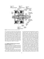
Figure 3.5 shows the “ANSYS Main Menu” window where we can find layered
command options imitating folders and files in the Microsoft® Explorer folder
window.
In order to prepare for creating the beam, the following operations should
be made:
(1) Click [A] Preprocessor to open its sub-menus in ANSYS Main Menu window.

(2) Click [B] Modeling to open its sub-menus and select Create menu.
(3) Click [C] Areas to open its sub-menus and select Rectangle menu.
(4) Click to select [D] By2cornersmenu.
Aftercarrying outthe operations above, awindow called Rectangle by2 corners as
shown in Figure 3.6 appears for the input of the geometry of a 2-D rectangular beam.
[2] Input of the beam geometry to analyze
The Rectangle by 2 corners window has four boxes for inputting the coordinates
of the lower left corner point of the rectangular beam and the width and height of
the beam to create. The following operations complete the creation procedure of the
beam:
(1) Input two 0’s into [A] WP X and [B] WP Y to determine the lower left corner
point of the beam on the Cartesian coordinates of the working plane.
(2) Input 0.09 and 0.005 (m) into [C] Width and [D] Height, respectively to
determine the shape of the beam model.
(3) Click [E] OK button to create the rectangular area, or beam on the ANSYS
Graphics window as shown in Figure 3.7.
Ch03-H6875.tex 24/11/2006 17: 2 page 55
3.1 Cantilever beam 55
A
B
C
D
Figure 3.5 “ANSYS Main Menu”
window.
A
B
C
D
E
Figure 3.6 “Rectangle By 2

Corners” window.
Figure 3.7 2-D beam created and displayed on the “ANSYS Graphics” window.
Ch03-H6875.tex 24/11/2006 17: 2 page 56
56 Chapter 3 Application of ANSYS to stress analysis
How to correct the shape of the model
In case of correcting the model, delete the area first, and repeat the procedures [1]
and [2] above. In order to delete the area, execute the following commands:
Command
ANSYS Main Menu →Preprocessor →Modeling →Delete →Area and Below
Then, the Delete Area and Below window opens and an upward arrow (↑) appears
on the ANSYS Graphics window:
(1) Move the arrow to the area to delete and click the left button of the mouse.
(2) The color of the area turns from light blue into pink.
(3) Click OK button and the area is to be deleted.
3.1.3.2 INPUT OF THE ELASTIC PROPERTIES OF THE BEAM MATERIAL
Next, we specify elastic constants of the beam. In the case of isotropic material,
the elastic constants are Young’s modulus and Poisson’s ratio. This procedure can be
performed anytime beforethe solutionprocedure,for instance,after settingboundary
conditions. If this procedure is missed, we cannot perform the solution procedure.
Command
ANSYS Main Menu →Preprocessor →Material Props →Material Models
Then the Define Material Model Behavior window opens as shown in
Figure 3.8:
A
E
Figure 3.8 “Define Material Model Behavior” window.
(1) Double-click [A] Structural, Linear, Elastic, and Isotropic buttons one after
another.
Ch03-H6875.tex 24/11/2006 17: 2 page 57
3.1 Cantilever beam 57

(2) Input the value of Young’s modulus, 2.1e11 (Pa), and that of Poisson’s ratio, 0.3,
into [B] EX and [C] PRXY boxes, and click [D] OK button of the LinearIsotropic
Properties for Material Number 1 as shown in Figure 3.9.

B
C
D
Figure 3.9 Input of elastic constants through the “Linear Isotropic Properties for Material Number 1”
window.
(3) Exit from the Define Material Model Behavior window by selecting Exit in [E]
Material menu of the window (see Figure 3.8).
3.1.3.3 F
INITE-ELEMENT DISCRETIZATION OF THE BEAM AREA
Here we will divide the beam area into finite elements. The procedures for finite-
element discretization are firstly to select the element type, secondly to input the
element thickness and finally to divide the beam area into elements.
[1] Selection of the element type
Command
ANSYS Main Menu →Preprocessor →Element Type →Add/ Edit/Delete
Then the Element Types window opens:
(1) Click [A] Add buttontoopentheLibrary of Element Types window as shown
in Figure 3.11 and select the element type to use.
(2) To select the 8-node isoparametric element, select [B] Structural Mass – Solid.
(3) Select [C] Quad 8node 82 and click [D] OK button to choose the 8-node
isoparametric element.
(4) Click [E] Options button in the Element Types window as shown in Fig-
ure 3.10 to open the PLANE82 element type options window as depicted in
Figure 3.12. Select [F] Plane strs w/thk item in the Element behavior box and
click [G] OK buttontoreturntotheElement Types window. Click [H] Close
button to close the window.

Ch03-H6875.tex 24/11/2006 17: 2 page 58
E
A
H
Figure 3.10 “Element Types” window.
D
B
C
Figure 3.11 “Library of Element Types” window.
F
G
Figure 3.12 “PLANE82 element type options” window.
Ch03-H6875.tex 24/11/2006 17: 2 page 59
3.1 Cantilever beam 59
Figure 3.13 8-node
isoparametric rectangu-
lar element.
A
Figure 3.14 Setting of the
element thickness from the real
constant command.
The 8-node isoparametric element is a rectan-
gular element which has four corner nodal points
and four middle points as shown in Figure 3.13 and
can realize the finite-element analysis with higher
accuracy than the 4-node linear rectangular ele-
ment. The beam area is divided into these 8-node
rectangular #82 finite elements.
[2] Input of the element thickness
Command

ANSYS Main Menu →Preprocessor →Real
Constants
Select [A] Real Constants in the ANSYS Main
Menu as shown in Figure 3.14.
(1) Click [A] Add/Edit/Delete buttontoopentheReal Constants window as shown
in Figure 3.15 and click [B] Add … button.
(2) Then the Element Type for Real Constants window opens (see Figure 3.16). Click
[C] OK button.
(3) The Element Type for Real Constants window vanishes and the Real Constants
Set Number 1. for PLANE82 window appears instead as shown in Figure 3.17.
B
Figure 3.15 “Real Constants” window
before setting the element thickness.
C
Figure 3.16 “Element Type for Real Constants”
window.
Ch03-H6875.tex 24/11/2006 17: 2 page 60
60 Chapter 3 Application of ANSYS to stress analysis
D
E
Figure 3.17 “Real Constants Set Number 1. for PLANE82” window.
Input a plate thickness of “0.01” (m) in [D] Thickness box and click [E] OK
button.
F
Figure 3.18 “Real Constants” window
after setting the element thickness.
(4) The Real Constants window returns
with the display of the Defined Real
Constants Sets box changed to Set 1
as shown in Figure 3.18. Click [F]

Close button, which makes the oper-
ation of setting the plate thickness
completed.
[3] Sizing of the elements
Command
ANSYS Main Menu →Preprocessor →
Meshing →Size Cntrls →Manual
Size →Global →Size
The Global Element Sizes window
opens as shown in Figure 3.19:
(1) Input 0.002 (m) in [A] SIZE box and
click [B] OK button.
By the operations above the element size of 0.002,i.e., 0.002 m,or 2 mmis specified
and the beam of 5 mm by 90 mm is divided into rectangular finite-elements with
one side 2 mm and the other side 3 mm in length.
[4] Meshing
Command
ANSYS Main Menu →Preprocessor →Meshing →Mesh →Areas →Free
The Mesh Areas window opens as shown in Figure 3.20:
(1) An upward arrow (↑) appears in the ANSYS Graphics window. Move this arrow
to the beam area and click this area to mesh.
(2) The color of the area turns from light blue into pink. Click [A] OK buttontosee
the area meshed by 8-node rectangular isoparametric finite elements as shown in
Figure 3.21.
Ch03-H6875.tex 24/11/2006 17: 2 page 61
3.1 Cantilever beam 61
A
B
Figure 3.19 “Global Element Sizes” window.
A

Figure 3.20 “Mesh Areas”
window.
Figure 3.21 Beam area subdivided into 8-node isoparametric rectangular
elements.
How to modify meshing
In case of modifying meshing, delete the elements, and repeat the procedures [1]
through [4]above. Repeatfrom theprocedures [1],from [2] or from[3] for modifying
the element type, for changing the plate thickness without changing the element type,
or for changing the element size only.
Ch03-H6875.tex 24/11/2006 17: 2 page 62
62 Chapter 3 Application of ANSYS to stress analysis
In order to delete the elements, execute the following commands:
Command
ANSYS Main Menu →Preprocessor →Meshing →Clear →Areas
The Clear Areas window opens:
(1) An upward arrow (↑) appears in the ANSYS Graphics window. Move this arrow
to the beam area and click this area.
(2) The color of the area turns from light blue into pink. Click OK buttontodeletethe
elements from the beam area. After this operation, the area disappears from the
display. Execute the following commands to replot the area.
Command
ANSYS Utility Menu →Plot →Areas
3.1.3.4 I
NPUT OF BOUNDARY CONDITIONS
Here we will impose constraint and loading conditions on nodes of the beam model.
Display the nodes first to define the constraint and loading conditions.
[1] Nodes display
Command
ANSYS Utility Menu →Plot →Nodes
The nodes are plotted in the ANSYS Graphics window opens as shown in Figure 3.22.

Figure 3.22 Plots of nodes.
Ch03-H6875.tex 24/11/2006 17: 2 page 63
3.1 Cantilever beam 63
[2] Zoom in the nodes display
Enlarged view of the models is often convenient when imposing constraint and load-
ing conditions on the nodes. In order to zoom in the node display, execute the
following commands:
Command
ANSYS Utility Menu →PlotCtrls →Pan Zoom Rotate
A
B
Figure 3.23 “Pan-Zoom-Rotate”
window.
The Pan-Zoom-Rotate window opens as shown
in Figure 3.23:
(1) Click [A] Box Zoom button.
(2) The shape of the mouse cursor turns into a
magnifying glass in the ANSYSGraphics win-
dow. Click the upper left point and then the
lower right point which enclose a portion of
the beam area to enlarge as shown in Figure
3.24. Zoom in the left end of the beam.
(3) In order to display the whole view of
the beam, click [B] Fit button in the
“Pan-Zoom-Rotate” window.
[3] Definition of constraint conditions
Selection of nodes
Command
ANSYS Main Menu →Solution →Define
Loads →Apply →Structural →

Displacement →On Nodes
The Apply U. ROT on Nodes window opens as
shown in Figure 3.25.
(1) Select [A] Box button and drag the mouse in
the ANSYS Graphics window so as to enclose
the nodes on the left edge of the beam area
with the yellow rectangular frame as shown
in Figure 3.26. The Box buttonisselected
to pick multiple nodes at once, whereas [B]
the “Single” button is chosen to pick a single
node.
(2) After confirming that only the nodes to
impose constraints on are selected, i.e., the
nodes on the left edge of the beam area, click
[C] OK button.
How to reselect nodes Click [D] Reset button to
clear the selection of the nodes before clicking [C]
OK button in the procedure (2) above, and repeat
the procedures (1) and (2) above. The selection of