Engineering Analysis with Ansys Software Episode 1 Part 7 potx

Ch03-H6875.tex 24/11/2006 17: 2 page 104
104 Chapter 3 Application of ANSYS to stress analysis
A
Figure 3.75 Applied stress on the right end side of the plate and resultant reaction force and longitudinal
stress in its ligament region.
defined as,
α
0
≡
σ
max
σ
0
=

1 +2
a
b

=

1 +

a
ρ

(3.5)
The stress concentration factor α
0
varies inversely proportional to the aspect ratio of
elliptic hole b/a, namely the smaller the value of the aspect ratio b/a or the radius

of curvature ρ becomes, the larger the value of the stress concentration factor α
0
becomes.
In a finite plate, the maximum stress at the foot of the hole is increased due to the
finite boundary of the plate. Figure3.76showsthe variation of the stressconcentration
factor α for elliptic holes having different aspect ratios with normalized major radius
2a/h, indicating that the stress concentration factor in a plate with finite width h is
increased dramatically as the ligament between the foot of the hole and the plate edge
becomes smaller.
From Figure 3.76, the value of the stress intensity factor for the present ellip-
tic hole is approximately 5.16, whereas Figure 3.75 shows that the maximum value
of the longitudinal stress obtained by the present FEM calculation is approxi-
mately 49.3 MPa, i.e., the value of the stress concentration factor is approximately
49.3/10 =4.93. Hence, the relative error of the present calculation is approximately,
(4.93 −5.16)/5.16 ≈−0.0446 =4.46% which may be reasonably small and so be
acceptable.
Ch03-H6875.tex 24/11/2006 17: 2 page 105
3.3 Stress concentration due to elliptic holes 105
0 0.2 0.4 0.6 0.8 1
0
5
10
15
20
Normalized major radius, 2a/h
Stress concentration factor, α
b/a=1.0
b/a=0.5
Aspect ratio
b/a=0.25

2a
2b
σ
0
σ
0
Figure 3.76 Variation of the stress concentration factor α for elliptic holes having different aspect ratios
with normalized major radius 2a/h.
3.3.5 Problems to solve
PROBLEM 3.8
Calculate the value of stress concentration factor for the elliptic hole shown in Fig-
ure 3.65 by using the whole model of the plate and compare the result with that
obtained and discussed in 3.3.4.
PROBLEM 3.9
Calculate the values of stress concentration factor α for circular holes for different
values of the normalized major radius 2a/h and plot the results as the α versus 2a/h
diagram as shown in Figure 3.76.
PROBLEM 3.10
Calculate the values of stress concentration factor α for elliptic holes having different
aspect ratios b/a for different values of the normalized major radius 2a/h and plot
the results as the α versus 2a/h diagram.
Ch03-H6875.tex 24/11/2006 17: 2 page 106
106 Chapter 3 Application of ANSYS to stress analysis
PROBLEM 3.11
For smaller values of 2a/h, the disturbance of stress in the ligament between the foot
of a hole andthe plate edge due to the existence of the hole isdecreased andstress inthe
ligament approaches to a constant value equal to the remote stress σ
0
at some distance
from the foot of the hole (remember the principle of St. Venant in the previous

section). Find how much distance from the foot of the hole the stress in the ligament
region can be considered to be almost equal to the value of the remote stress σ
0
.
3.4 Stress singularity problem
3.4.1 Example Problem
An elastic plate with a crack of length 2a in its center subjected touniform longitudinal
tensile stress σ
0
at one end and clamped at the other end as illustrated in Figure 3.77.
Perform an FEM analysis of the 2-D elastic center-cracked tension plate illustrated
in Figure 3.77 and calculate the value of the mode I (crack-opening mode) stress
intensity factor for the center-cracked plate.
Uniform longitudinal stress σ0
400 mm
200 mm
200 mm
B
A
100 mm
20 mm
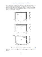
Figure 3.77 Two dimensional elastic plate with a crack of length 2a in its center subjected to a uniform
tensile stress σ
0
in the longitudinal direction at one end and clamped at the other end.
3.4.2 Problem description
Specimen geometry: length l =400 mm, height h =100 mm.
Material: mild steel having Young’s modulus E =210 GPa and Poisson’s ratio ν =0.3.
Ch03-H6875.tex 24/11/2006 17: 2 page 107
3.4 Stress singularity problem 107

Crack: A crack is placed perpendicular to the loading direction in the center of the
plate and has a length of 20 mm. The center-cracked tension plate is assumed to be
in the plane strain condition in the present analysis.
Boundary conditions: The elastic plate is subjected to a uniform tensile stress in the
longitudinal direction at the right end and clamped to a rigid wall at the left end.
3.4.3 Analytical procedures
3.4.3.1 CREATION OF AN ANALYTICAL MODEL
Let us use a quarter model of the center-cracked tension plate as illustrated in
Figure 3.77, since the plate is symmetric about the horizontal and vertical center lines.
Here we use the singular element or the quarter point element which can inter-
polate the stress distribution in the vicinity of the crack tip at which stress has the
1/
√
r singularity where r is the distance from the crack tip (r/a << 1). An ordinary
isoparametric element which is familiar to you as “Quad 8node 82” has nodes at the
corners and also at the midpoint on each side of the element. A singular element,
however, has the midpoint moved one-quarter side distance from the original mid-
point position to the node which is placed at the crack tip position. This is the reason
why the singular element is often called the quarter point element instead. ANSYS
software is equipped only with a 2-D triangular singular element, but neither with
2-D rectangular nor with 3-D singular elements. Around the node at the crack tip, a
circular area is created and is divided into a designated number of triangular singular
elements. Each triangular singular element has its vertex placed at the crack tip posi-
tion and has the quarter points on the two sides joining the vertex and the other two
nodes.
In order to create the singular elements, the plate area must be created via key-
points set at the four corner points and at the crack tip position on the left-end side
of the quarter plate area.
Command
ANSYS Main Menu →Preprocessor →Modeling →Create →Keypoints →

In Active CS
(1) The Create Keypoints in Active Coordinate System window opens as shown in
Figure 3.78.
(2) Input [A] each keypoint number in the NPT box and [B] x-, y-, and z-
coordinates of each keypoint in the three X, Y, Z boxes, respectively. Figure
3.78 shows the case of Key point #5, which is placed at the crack tip having the
coordinates (0, 10, 0). In the present model, let us create Key points #1 to #5 at the
coordinates (0, 0, 0), (200, 0, 0), (200, 50, 0), (0, 50, 0), and (0, 10, 0), respectively.
Note that the z-coordinate is always 0 in 2-D elasticity problems.
(3) Click [C] Apply button four times and create Key points #1 to #4 without exiting
from the window and finally click [D] OK button to create key point #5 at the
crack tip position and exit from the window (see Figure 3.79).
Then create the plate area via the five key points created in the procedures above
by the following commands:
Ch03-H6875.tex 24/11/2006 17: 2 page 108
108 Chapter 3 Application of ANSYS to stress analysis
A
B
C
D
Figure 3.78 “Create Keypoints in Active Coordinate System” window.
Figure 3.79 Five key points created in the “ANSYS Graphics” window.
Command
ANSYS Main Menu →Preprocessor →Modeling →Create →Areas →
Arbitrary →Through KPs
(1) The Create Area thru KPs window opens.
(2) The upward arrow appears in the ANSYS Graphics window. Move this arrow to
Key point #1 and click this point. Click Key points #1 through #5 one by one
counterclockwise (see Figure 3.80).
(3) Click the OK button to create the plate area as shown in Figure 3.81.

Ch03-H6875.tex 24/11/2006 17: 2 page 109
3.4 Stress singularity problem 109
Figure 3.80 Clicking Key points #1 through #5 one by one counterclockwise to create the plate area.
Figure 3.81 Quarter model of the center cracked tension plate.
Ch03-H6875.tex 24/11/2006 17: 2 page 110
110 Chapter 3 Application of ANSYS to stress analysis
3.4.3.2 INPUT OF THE ELASTIC PROPERTIES OF THE PLATE MATERIAL
Command
ANSYS Main Menu →Preprocessor →Material Props →Material Models
(1) The Define Material Model Behavior window opens.
(2) Double-click Structural, Linear, Elastic, and Isotropic buttons one after
another.
(3) Input the value of Young’s modulus, 2.1e5 (MPa), and that of Poisson’s ratio,
0.3, into EX and PRXY boxes, and click the OK button of the Linear Isotropic
Properties for Materials Number 1 window.
(4) Exit from the Define Material Model Behavior window by selecting Exit in the
Material menu of the window.
3.4.3.3 FINITE-ELEMENT DISCRETIZATION OF THE CENTER-CRACKED
TENSION PLATE AREA
[1] Selection of the element type
Command
ANSYS Main Menu →Preprocessor →Element Type →Add/Edit/Delete
(1) The Element Types window opens.
(2) Click the Add … button in the Element Types window to open the Library of
Element Types window and select the element type to use.
(3) Select Structural Mass – Solid and Quad 8 node 82.
(4) Click the OK button in the Library of Element Types window to use the 8-node
isoparametric element.
(5) Click the Options … button in the Element Types window to open the
PLANE82 element type options window. Select the Plane strain item in the

Element behavior box and click the OK buttontoreturntotheElement Types
window. Click the Close button in the Element Types window to close the
window.
[2] Sizing of the elements
Before meshing, the crack tip point around which the triangular singular elements
will be created must be specified by the following commands:
Command
ANSYS Main Menu →Preprocessor →Meshing →Size Cntrls →
Concentrate KPs →Create
(1) The Concentration Keypoint window opens.
(2) Display the key points in the ANSYS Graphics window by
Command
ANSYS Utility Menu →Plot →Keypoints →Keypoints.
Ch03-H6875.tex 24/11/2006 17: 2 page 111
3.4 Stress singularity problem 111
(3) Pick Key point #5 by placing the upward arrow onto Key point #5 and by clicking
the left button of the mouse. Then click the OK button in the Concentration
Keypoint window.
(4) Another Concentration Keypoint window opens as shown in Figure 3.82.
A
B
C
D
E
F
Figure 3.82 “Concentration Keypoint” window.
(5) Confirming that [A] 5, i.e., the key point number of the crack tip position is
input in the NPT box, input [B] 2 in the DELR box, [C] 0.5 in the RRAT box
and [D] 6 in the NTHET box and select [E] Skewed 1/4pt in the KCTIP box in
the window. Refer to the explanations of the numerical data described after the

names of the respective boxes on the window. Skewed 1/4pt in the last box means
that the mid nodes of the sides of the elements which contain Key point #5 are
the quarter points of the elements.
(6) Click [F] OK button in the Concentration Keypoint window.
The size of the meshes other than the singular elements and the elements adjacent
to them can be controlled by the same procedures as have been described in the
previous sections of the present Chapter 3.
Command
ANSYS Main Menu →Preprocessor →Meshing →Size Cntrls →Manual Size →
Global →Size
(1) The Global Element Sizes window opens.
(2) Input 1.5 in the SIZE box and click the OK button.
[3] Meshing
The meshing procedures are also the same as before.
Command
ANSYS Main Menu →Preprocessor →Meshing →Mesh →Areas →Free
Ch03-H6875.tex 24/11/2006 17: 2 page 112
112 Chapter 3 Application of ANSYS to stress analysis
(1) The Mesh Areas window opens.
(2) The upward arrow appears in the ANSYS Graphics window. Move this arrow to
the quarter plate area and click this area.
(3) The color of the area turns from light blue into pink. Click the OK button.
(4) The Warning window appears as shown in Figure 3.83 due to the existence of
six singular elements. Click [A] Close button and proceed to the next operation
below.
A
Figure 3.83 “Warning” window.
(5) Figure 3.84 shows the plate area meshed by ordinary 8-node isoparametric finite
elements except for the vicinity of the crack tip where we have six singular
elements.

Figure 3.84 Plate area meshed by ordinary 8-node isoparametric finite elements and by singular elements.
Ch03-H6875.tex 24/11/2006 17: 2 page 113
3.4 Stress singularity problem 113
Figure 3.85 is an enlarged view of the singular elements around [A] the crack
tip showing that six triangular elements are placed in a radial manner and that the
size of the second row of elements is half the radius of the first row of elements, i.e.,
triangular singular elements.
A
Figure 3.85 Enlarged view of the singular elements around the crack tip.
3.4.3.4 INPUT OF BOUNDARY CONDITIONS
[1] Imposing constraint conditions on the ligament region of the left end
and the bottom side of the quarter plate model
Due to the symmetry, the constraint conditions of the quarter plate model are
UX-fixed condition on the ligament region of the left end, that is, the line between
Key points #4 and #5, and UY-fixed condition on the bottom side of the quarter
plate model. Apply these constraint conditions onto the corresponding lines by the
following commands:
Command
ANSYS Main Menu →Solution →Define Loads →Apply →Structural →
Displacement →On Lines
(1) The Apply U. ROT on Lines window opens and the upward arrow appears when
the mouse cursor is moved to the ANSYS Graphics window.
(2) Confirming that the Pick and Single buttons are selected, move the upward arrow
onto the line between Key points #4 and #5 and click the left button of the mouse.
(3) Click the OK button in the Apply U. ROT on Lines window to display another
Apply U. ROT on Lines window.
Ch03-H6875.tex 24/11/2006 17: 2 page 114
114 Chapter 3 Application of ANSYS to stress analysis
(4) Select UX in the Lab2 box and click the OK button in the Apply U. ROT on Lines
window.

Repeat the commands and operations (1) through (3) above for the bottom side
of the model. Then, select UY in the Lab2 box and click the OK button in the Apply
U. ROT on Lines window.
[2] Imposing a uniform longitudinal stress on the right end of the quarter
plate model
A uniform longitudinal stress can be defined by pressure on the right-end side of the
plate model as described below:
Command
ANSYS Main Menu →Solution →Define Loads →Apply →Structural →
Pressure →On Lines
(1) The Apply PRES on Lines window opens and the upward arrow appears when
the mouse cursor is moved to the ANSYS Graphics window.
(2) Confirming that the Pick and Single buttons are selected, move the upward arrow
onto the right-end side of the quarter plate area and click the left button of the
mouse.
(3) Another Apply PRES on Lines window opens. Select Constant value in the [SFL]
Apply PRES on lines as a box and input −10 (MPa) in the VALUE Load PRES
value box and leave a blank in the Va l ue box.
(4) Click the OK button in the window to define a uniform tensile stress of 10 MPa
applied to the right end of the quarter plate model.
Figure 3.86 illustrates the boundary conditions applied to the center-cracked
tension plate model by the above operations.
3.4.3.5 SOLUTION PROCEDURES
The solution procedures are also the same as usual.
Command
ANSYS Main Menu →Solution →Solve →Current LS
(1) The Solve Current Load Step and /STATUS Command windows appear.
(2) Click the OK button in the SolveCurrent Load Step window to begin the solution
of the current load step.
(3) The Verify window opens as shown in Figure 3.87. Proceed to the next operation

below by clicking [A] Yes button in the window.
(4) Select the File button in /STATUS Command window to open the submenu and
select the Close button to close the /STATUS Command window.
(5) When the solutionis completed, the Note window appears. Click the Close button
to close the Note window.
Ch03-H6875.tex 24/11/2006 17: 2 page 115
3.4 Stress singularity problem 115
Figure 3.86 Boundary conditions applied to the center-cracked tension plate model.
A
Figure 3.87 “Verify” window.
3.4.3.6 CONTOUR PLOT OF STRESS
Command
ANSYS Main Menu →General Postproc →Plot Results →Contour Plot →Nodal
Solution
(1) The Contour Nodal Solution Data window opens.
(2) Select Stress and X-Component of stress.
(3) Select Deformed shape with deformed edge in the Undisplaced shape key box
to compare the shapes of the cracked plate before and after deformation.
(4) Click the OK button to display the contour of the x-component of stress, or
longitudinal stress in the center-cracked tension plate in the ANSYS Graphics
window as shown in Figure 3.88.
Ch03-H6875.tex 24/11/2006 17: 2 page 116
116 Chapter 3 Application of ANSYS to stress analysis
Figure 3.88 Contour of the x-component of stress in the center-cracked tension plate.
Figure 3.89 is an enlarged view of the longitudinal stress distribution around the
crack tip showing that very high tensile stress is induced at the crack tip whereas
almost zero stress around the crack surface and that the crack shape is parabolic.
3.4.4 Discussion
Figure 3.90 shows extrapolation of the values of the correction factor, or the non-
dimensional mode I (the crack-opening mode) stress intensity factor F

I
=K
I
/(σ
√
πa)
to the point where r =0, that is, the crack tip position by the hybrid extrapolation
method [1]. The plots in the right region of the figure are obtained by the formula:
K
I
= lim
r→0
√
2πrσ
x
(θ = 0) (3.6)
or
F
I
(λ) =
K
I
σ
√
πa
= lim
r→0
√
πrσ
x

(θ = 0)
√
hσ
√
πλ
where λ = 2a/h (3.6

)
whereas those in the left region
K
I
= lim
r→0

2π
r
E
(1 +ν)(κ +1)
u
x
(θ = π) (3.7)
or
F
I
(λ) =
K
I
σ
√
πa

= lim
r→0

π
hr
E
(1 +ν)(κ +1)σ
√
πλ
u
x
(θ = π) (3.7

)
Ch03-H6875.tex 24/11/2006 17: 2 page 117
3.4 Stress singularity problem 117
Figure 3.89 Enlarged view of the longitudinal stress distribution around the crack tip.
20246
0
1
2
F
I
ϭ 1.0200
Distance from the crack tip (mm)
r
r/3
Correction factor, (F
I
=K

I
/(σ√πa)
Hybrid interpolation method
Displacement
Stress
Crack
CCT Plate
λ ≡ 2a/h ϭ 0.2
Figure 3.90 Extrapolation of the values of the correction factor F
I
=K
I
/(σ
√
πa) to the crack tip point
where r =0.
where r is the distance from the crack tip, σ
x
(θ =0) the x-component of stress at
θ =0, i.e., along the ligament, σ the applied uniform stress in the direction of the
x-axis, a the half crack length, E Young’s modulus, u
x
(θ =π) the x-component of
strain at θ =π, i.e., along the crack surface, κ =3−4 ν for plane strain condition and
κ =(3−ν)/(1 +ν) for plane stress condition and θ the angle around the crack tip. The
correction factor F
I
accounts for the effect of the finite boundary, or the edge effect of
the plate. The value of F
I

can be evaluated either by the stress extrapolation method
Ch03-H6875.tex 24/11/2006 17: 2 page 118
118 Chapter 3 Application of ANSYS to stress analysis
(the right region) or by the displacement extrapolation method (the left region). The
hybrid extrapolation method [1] is a blend of the two types of the extrapolation
methods above and can bring about better solutions. As illustrated in Figure 3.90,
the extrapolation lines obtained by the two methods agree well with each other when
the gradient of the extrapolation line for the displacement method is rearranged by
putting r

=r/3. The value of F
I
obtained for the present CCT plate by the hybrid
method is 1.0200.
Table 3.1 Correction factor F
I
(λ) as a function of non-dimensional crack length λ =2a/h
λ =2a/h Isida Feddersen Koiter Tada
Equation (3.8) Equation (3.9) Equation (3.10) Equation (3.11)
0.1 1.0060 1.0062 1.0048 1.0060
0.2 1.0246 1.0254 1.0208 1.0245
0.3 1.0577 1.0594 1.0510 1.0574
0.4 1.1094 1.1118 1.1000 1.1090
0.5 1.1867 1.1892 1.1757 1.1862
0.6 1.3033 1.3043 1.2921 1.3027
0.7 1.4882 1.4841 1.4779 1.4873
0.8 1.8160 1.7989 1.8075 1.8143
0.9 2.5776 – 2.5730 2.5767
Table 3.1 lists the values of F
I

calculated by the following four equations [2–6] for
various values of non-dimensional crack length λ =2a/h:
F
I
(λ) = 1 +
35

k=1
A
k
λ
2k
(3.8)
F
I
(λ) =

sec(πλ/2) (λ ≤ 0.8) (3.9)
F
I
(λ) =
1 −0.5λ +0.326λ
2
√
1 −λ
(3.10)
F
I
(λ) = (1 −0.025λ
2

+0.06λ
4
)

sec(πλ/2) (3.11)
Among these, Isida’s solution is considered to be the best. The value of
F
I
(0.2) by Isida is 1.0246. The relative error of the present result is (1.0200 −
1.0246)/1.0246 =−0.45%, which is a reasonably good result.
3.4.5 Problems to solve
PROBLEM 3.12
Calculate the values of the correction factor for the mode I stress intensity factor for
the center-cracked tension plate having normalized crack lengths of λ =2a/h =0.1
Ch03-H6875.tex 24/11/2006 17: 2 page 119
3.4 Stress singularity problem 119
to 0.9. Compare the results with the values of the correction factor F(λ) listed in
Table 3.1
PROBLEM 3.13
Calculate the values of the correction factor for the mode I stress intensity factor for a
double edge cracked tension plate having normalized crack lengths of λ =2a/h =0.1
to 0.9 (see Figure P3.13). Compare the results with the values of the correction factor
F(λ) calculated by Equation (P3.13) [7, 8]. Note that the quarter model described in
the present section can be used for the FEM calculations of this problem simply by
changing the boundary conditions.
F
I
(λ) =
1.122 −0.561λ −0.205λ
2

+0.471λ
3
−0.190λ
4
√
1 −λ
where λ = 2a/h
(P3.13)
Uniform longitudinal stress σ
0
200 mm200 mm
400 mm
h = 100
a
a
Figure P3.13 Double edge cracked tension plate subjected to a uniform longitudinal stress at one end and
clamped at the other end.
PROBLEM 3.14
Calculate the values of the correction factor for the mode I stress intensity factor for
a single edge cracked tension plate having normalized crack lengths of λ =2a/h =0.1
to 0.9 (see Figure P3.14). Compare the results with the values of the correction factor
F(λ) calculated by Equation (P3.14) [7, 9]. In this case, a half plate model which is
clamped along the ligament and is loaded at the right end of the plate. Note that the
whole plate model with an edge crack needs a somewhat complicated procedure. An
Ch03-H6875.tex 24/11/2006 17: 2 page 120
120 Chapter 3 Application of ANSYS to stress analysis
Uniform longitudinal stress σ
0
400 mm
200 mm 200 mm

h ϭ 100
a
Figure P3.14 Single edge cracked tension plate subjected to a uniform longitudinal stress at one end and
clamped at the other end.
approximate model as described above gives good solutions with an error of a few
percent or less and is sometimes effective in practice.
F
I
(λ) =
0.752 +2.02λ +0.37[1 −sin(πλ/2)]
3
cos(πλ/2)

2
πλ
tan

πλ
2

where λ = a/h
(P3.14)
3.5 Two-dimensional contact stress
3.5.1 Example problem
An elastic cylinder of mild steel with a radius of R pressed against a flat surface of a
linearly elastic medium of the same material by a force P’. Perform an FEM analysis
of the elastic cylinder pressed against the elastic flat plate illustrated in Figure 3.91
and calculate the resulting contact stress in the vicinity of the contact point in the flat
plate.
3.5.2 Problem description

Geometry of the cylinder: radius R =1000 mm.
Geometry of the flat plate: width W =1000 mm, height h =500 mm.
Material: mild steel having Young’s modulus E =210 GPa and Poisson’s ratio ν =0.3.
Boundary conditions: The elastic cylinder is pressed against the elastic flat plate
by a force of P’ =1 kN/mm and the plate is clamped at the bottom. Note that the
cylinder and the plate is considered to have an unit thickness in the case of plane
stress condition.
Ch03-H6875.tex 24/11/2006 17: 2 page 121
3.5 Two-dimensional contact stress 121
500 mm

P’
R=500 mm
500 mm
500 mm
P/2
R=500mm
1000 mm
Figure 3.91 Elastic cylinder of mild steel with a radius of R pressed against an elastic flat plate of the same
steel by a force P’ and the FEM model of the cylinder-plate system.
3.5.3 Analytical procedures
3.5.3.1 CREATION OF AN ANALYTICAL MODEL
Let us use a half model of the indentation problem illustrated in Figure 3.91, since
the problem is symmetric about the vertical center line.
[1] Creation of an elastic flat plate
Command
ANSYS Main Menu →Preprocessor →Modeling →Create →Areas →
Rectangle →By2Corners
(1) Input two 0’s into the WP X and WP Y boxes in the Rectangle by 2 Corners
window to determine the upper left corner point of the elastic flat plate on the

Cartesian coordinates of the working plane.
(2) Input 500 and −500 (mm) into the Width and Height boxes, respectively, to
determine the shape of the elastic flat plate model.
(3) Click the OK button to create the plate on the ANSYS Graphics window.
[2] Creation of an elastic cylinder
Command
ANSYS Main Menu →Preprocessor →Modeling →Create →Areas →
Circle →Partial Annulus
Ch03-H6875.tex 24/11/2006 17: 2 page 122
122 Chapter 3 Application of ANSYS to stress analysis
A
B
C
D
E
F
G
Figure 3.92 “Part Annular Circ
Area” window.
(1) The Part Annular Circ Area window
opens as shown in Figure 3.92.
(2) Input 0and 500 into[A] WPX and[B] WP
Y boxes, respectively, in the Part Annular
Circ Area window to determine the cen-
ter of the elastic cylinder on the Cartesian
coordinates of the working plane.
(3) Input two 500’s (degree) into [C] Rad-1
and [E]Rad-2 boxesto designatethe radius
of the elastic cylinder model.
(4) Input −90 and 0 (mm) into [D] Theta-

1 and [F] Theta-2 boxes, respectively, to
designate the starting and ending angles of
the quarter elastic cylinder model.
(5) Click [G] OK button to create the quarter
cylinder model on the ANSYS Graphics
window as shown in Figure 3.93.
[3] Combining the elastic cylinder and the
flat plate models
The elastic cylinder and the flat plate models
must be combined into one model so as not
to allow the rigid-body motions of the two
bodies.
Figure 3.93 Areas of the FEM model for an elastic cylinder pressed against an elastic flat plate.
Ch03-H6875.tex 24/11/2006 17: 2 page 123
3.5 Two-dimensional contact stress 123
Command
A
Figure 3.94 “Glue Areas”
window.
ANSYS Main Menu →Preprocessor →
Modeling →Operate →Booleans →Glue →
Areas
(1) The Glue Areas window opens as shown in
Figure 3.94.
(2) The upward arrow appears in the ANSYS
Graphics window. Move this arrow to the
quarter cylinder area and click this area, and
then move the arrow on to the half plate area
and click this area to combine these two areas.
(3) Click [A] OK button to create the contact

model on the ANSYS Graphics window as
shown in Figure 3.93.
3.5.3.2 INPUT OF THE ELASTIC PROPERTIES
OF THE MATERIAL FOR THE
CYLINDER AND THE FLAT PLATE
Command
ANSYS Main Menu →Preprocessor →
Material Props →Material Models
(1) The Define Material Model Behavior win-
dow opens.
(2) Double-click Structural, Linear, Elastic, and
Isotropic buttons one after another.
(3) Input the value of Young’s modulus, 2.1e5 (MPa), and that of Poisson’s ratio,
0.3, into EX and PRXY boxes, and click the OK button of the Linear Isotropic
Properties for Materials Number 1 window.
(4) Exit from the Define Material Model Behavior window by selecting Exit in the
Material menu of the window.
3.5.3.3 F
INITE-ELEMENT DISCRETIZATION OF THE CYLINDER AND THE
FLAT PLATE AREAS
[1] Selection of the element types
Select the 8-node isoparametric elements as usual.
Command
ANSYS Main Menu →Preprocessor →Element Type →Add/Edit/Delete
(1) The Element Types window opens.
(2) Click the Add … button in the Element Types window to open the Library of
Element Types window and select the element type to use.