Engineering Analysis with Ansys Software Episode 1 Part 9 pdf
Bạn đang xem bản rút gọn của tài liệu. Xem và tải ngay bản đầy đủ của tài liệu tại đây (1.37 MB, 20 trang )
Ch04-H6875.tex 24/11/2006 17: 47 page 144
144 Chapter 4 Mode analysis
(a) (b) (c)
Figure 4.1 FEM element types: (a) beam element; (b) shell element; and (c) solid element.
4.2 Mode analysis of a straight bar
4.2.1
Problem description
Obtain the lowest three vibration modes and resonant frequencies in the y direction
of the straight steel bar shown in Figure 4.2.
10 mm
x (mm)
20 40 60 80
Cross section
5mm
100
y
Figure 4.2 Cantilever beam for mode analysis.
Thickness of the bar is 0.005 m, width is 0.01 m, and the length is 0.09 m. Material
of the bar is steel with Young’s modulus, E =206 GPa, and Poisson’s ratio ν =0.3.
Density ρ =7.8 ×10
3
kg/m
3
.
Boundary condition: All freedoms are constrained at the left end.
4.2.2
Analytical solution
Before mode analysis is attempted using ANSYS program, an analytical solution for
resonant frequencies will be obtained to confirm the validity of ANSYS solution. The
analytical solution of resonant frequencies for a cantilever beam in y direction is
given by:
f
i
=
λ
2
i
2πL
2
EI
M
(i = 1, 2, 3, ) (4.1)
where length of the cantilever beam, L =0.09 m, cross-section area of the cantilever
beam, A =5 ×10
−5
m
2
, and Young’s modulus, E =206 GPa.
Ch04-H6875.tex 24/11/2006 17: 47 page 145
4.2 Mode analysis of a straight bar 145
The area moment of inertia of the cross-section of the beam is:
I = bt
3
/12 = (0.01 ×0.005
3
)/12 = 1.042 ×10
−10
m
4
Mass per unit width M =ρAL/L =ρA=7.8×10
3
kg/m
3
×5×10
−5
m
2
=0.39kg/m
λ
1
= 1.875 λ
2
= 4.694 λ
3
= 7.855.
For that set of data the following solutions are obtained: f
1
=512.5 Hz, f
2
=3212 Hz,
and f
3
=8994 Hz.
Figure 4.3 shows the vibration modes and the positions of nodes obtained by
Equation (4.1).
0.744 L 0.5 L
0.868 Li ϭ 1 i ϭ 2 i ϭ 3
Figure 4.3 Analytical vibration mode and the node position.
i
j
θ
j
x
j
y
j
y
i
x
i
θ
i
Figure 4.4 Two -
dimensional beam
element.
4.2.3 Model for finite-element analysis
4.2.3.1 ELEMENT TYPE SELECTION
In FEM analysis, it is very important to select a proper element type which influences
the accuracy of solution, working time for model construction, and CPU time. In this
example, the two-dimensional elastic beam, as shown in Figure 4.4, is selected for the
following reasons:
(a) Vibration mode is constrained in the two-dimensional plane.
(b) Number of elements can be reduced; the time for model construction and CPU
time are both shortened.
Two-dimensional elastic beam has three degrees of freedom at each node (i, j), which
are translatory deformations in the x and y directions and rotational deformation
around the z-axis. This beam can be subjected to extension or compression bend-
ing due to its length and the magnitude of the area moment of inertia of its cross
section.
Command
ANSYS Main Menu →Preprocessor →Element Type →Add/Edit/Delete
Then the window Element Types, as shown in Figure 4.5, is opened.
(1) Click [A]Add. Then the window Library of ElementTypes as shown in Figure 4.6
opens.
Ch04-H6875.tex 24/11/2006 17: 47 page 146
146 Chapter 4 Mode analysis
A
Figure 4.5 Window of Element Types.
D
B
C
Figure 4.6 Window of Library of Element Types.
(2) Select [B] Beam in the table Library of Element Types and, then, select [C] 2D
elastic 3.
(3) Element type reference number is set to 1 and click D OK button. Then the
window Library of Element Types is closed.
(4) Click [E] Close button in the window of Figure 4.7.
Ch04-H6875.tex 24/11/2006 17: 47 page 147
4.2 Mode analysis of a straight bar 147
E
Figure 4.7 Window of Library of Element Types.
4.2.3.2 REAL CONSTANTS FOR BEAM ELEMENT
Command
ANSYSMain Menu →Preprocessor →Real Constants →Add/Edit/Delete →Add
(1) The window Real Constants opens. Click [A] add button, and the window
Element Type for Real Constants appears in which the name of element type
selected is listed as shown in Figure 4.8.
(2) Click [B] OK button to input the values of real constants and the window Real
Constant for BEAM3 is opened (Figure 4.9).
(3) Input the following values in Figure 4.10. [C] Cross-sectional area =5e−5;
[D] Area moment of inertia =1.042e−10; [E] Total beam height =0.005. After
inputting these values, click [F] OK button to close the window.
(4) Click [G] Close button in the window Real Constants (Figure 4.11).
4.2.3.3 M
ATERIAL PROPERTIES
This section describes the procedure of defining the material properties of the beam
element.
Command
ANSYS Main Menu →Preprocessor →Material Props →Material Models
(1) Click the above buttons in the specified order and the window Define Material
Model Behavior opens (Figure 4.12).
Ch04-H6875.tex 24/11/2006 17: 47 page 148
148 Chapter 4 Mode analysis
A
Figure 4.8 Window of Real Constants.
B
Figure 4.9 Window of Element Type for
Real Constants.
D
E
C
F
Figure 4.10 Window of Real Constants for BEAM3.
Ch04-H6875.tex 24/11/2006 17: 47 page 149
4.2 Mode analysis of a straight bar 149
G
Figure 4.11 Window of Real Constants.
(2) Double click the following terms in the window.
[A] Structural →Linear →Elastic →Isotropic.
As a result the window Linear Isotropic Properties for Material Number 1 opens
(Figure 4.13).
(3) Input Young’s modulus of 206e9 to [B] EX box and Poisson ratio of 0.3 to [C]
PRXY box. Then click [D] OK button.
Next, define the value of density of material.
(1) Double click the term of Density in Figure 4.12 and the window Density for
Material Number 1 opens (Figure 4.14).
(2) Input the value of density,7800 to [F] DENS box and click [G] OK button. Finally,
close the window Define Material Model Behavior by clicking [H] X mark at the
upper right corner (Figures 4.12 and 4.14).
4.2.3.4 CREATE KEYPOINTS
To draw a cantilever beam for analysis, the method of using keypoints is described.
Command
ANSYS Main Menu →Preprocessor →Modeling →Create Keypoints →
In Active CS
The window Create Keypoints in Active Coordinate System opens.
Ch04-H6875.tex 24/11/2006 17: 47 page 150
150 Chapter 4 Mode analysis
A
E
H
Figure 4.12 Window of Define Material Model Behavior.
D
C
B
Figure 4.13 Window of Linear Isotropic Properties for Material Number 1.
(1) Input 1 to [A] NPT KeyPoint number box, 0,0,0 to [B] X, Y, Z Location in
active CS box, and then click [C] Apply button. Do not click OK button at this
stage. If you click OK button, the window will be closed. In this case, open the
window Create Keypoints in Active Coordinate System and then proceed to
step 2 (Figure 4.15).
Ch04-H6875.tex 24/11/2006 17: 47 page 151
4.2 Mode analysis of a straight bar 151
F
G
Figure 4.14 Window of Density for Material Number 1.
A
B
C
Figure 4.15 Window of Create Keypoint in Active Coordinate System.
(2) In the same window, input 2 to [D] NPT Keypoint number box, 0.09, 0,0
to [E] X, Y, Z Location in active CS box, and then click [F] OK button
(Figure 4.16).
(3) After finishing the above steps, two keypoints appear in the window (Figure 4.17).
4.2.3.5 C
REATE A LINE FOR BEAM ELEMENT
By implementing the following steps, a line between two keypoints is created.
Command
ANSYS Main Menu →Preprocessor →Modeling →Create →Lines →Lines→
Straight Line
Ch04-H6875.tex 24/11/2006 17: 47 page 152
152 Chapter 4 Mode analysis
D
E
F
Figure 4.16 Window of Create Keypoint in Active Coordinate System.
Figure 4.17 ANSYS Graphics window.
The window Create Straight Line, as shown in Figure 4.18, is opened.
(1) Pick the keypoints [A] 1 and [B] 2 (as shown in Figure 4.19) and click [C] OK
button in the window Create Straight Line (as shown in Figure 4.18). A line is
created.
4.2.3.6 CREATE MESH IN A LINE
Command
ANSYS Main Menu →Preprocessor →Meshing →Size Cntrls →Manual
Size →Lines →All Lines
Ch04-H6875.tex 24/11/2006 17: 47 page 153
C
Figure 4.18 Window of Create Straight Line.
A
B
Figure 4.19 ANSYS Graphics window.
Ch04-H6875.tex 24/11/2006 17: 47 page 154
154 Chapter 4 Mode analysis
The window Element Sizes on All Selected Lines, as shown in Figure 4.20, is
opened.
(1) Input [A] the number of 20 to NDIV box. This means that a line is divided into
20 elements.
(2) Click [B] OK button and close the window.
A
B
Figure 4.20 Window of Element Sizes on All Selected Lines.
From ANSYS Graphics window, the preview of the divided line is available, as
shown in Figure 4.21, but the line is not really divided at this stage.
Command
ANSYS Main Menu →Preprocessor →Meshing →Mesh →Lines
The window Mesh Lines, as shown in Figure 4.22, opens.
(1) Click [C] the line shown in ANSYS Graphics window and, then, [D] OK button
to finish dividing the line.
4.2.3.7 BOUNDARY CONDITIONS
The left end of nodes is fixed in order to constrain the left end of the cantilever
beam.
Command
ANSYS Main Menu → Solution → Define Loads → Apply → Structural →
Displacement →On Nodes.
Ch04-H6875.tex 24/11/2006 17: 47 page 155
C
Figure 4.21 Preview of the divided line.
D
Figure 4.22 Window of Mesh Lines.
B
Figure 4.23 Window of Apply
U,ROTonNodes.
Ch04-H6875.tex 24/11/2006 17: 47 page 156
156 Chapter 4 Mode analysis
The window Apply U,ROT on Nodes, as shown in Figure 4.23, opens.
(1) Pick [A] the node at the left end in Figure 4.24 and click [B] OK button. Then the
window Apply U,ROT on Nodes as shown in Figure 4.25 opens.
(2) In order to set the boundary condition, select [C] All DOF in the box Lab2. In the
box VAL U E [D] input 0 and, then, click [E] OK button. After these steps, ANSYS
Graphics window is changed as shown in Figure 4.26.
A
Figure 4.24 ANSYS Graphics window.
0
E
D
C
Figure 4.25 Window of Apply U,ROT on Nodes.
Ch04-H6875.tex 24/11/2006 17: 47 page 157
4.2 Mode analysis of a straight bar 157
Figure 4.26 Window after the boundary condition was set.
4.2.4 Execution of the analysis
4.2.4.1 DEFINITION OF THE TYPE OF ANALYSIS
The following steps are used to define the type of analysis.
Command
ANSYS Main Menu →Solution →Analysis Type →New Analysis
The window New Analysis, as shown in Figure 4.27, opens.
(1) Check [A] Modal and, then, click [B] OK button.
In order to define the number of modes to extract, the following procedure is
followed.
Command
ANSYS Main Menu →Solution →Analysis Type →Analysis Options
The window Modal Analysis, as shown in Figure 4.28, opens.
(1) Check [C] Subspace of MODOPT and input [D] 3 in the box of No. of modes
to extract and click [E] OK button.
Ch04-H6875.tex 24/11/2006 17: 47 page 158
158 Chapter 4 Mode analysis
A
B
Figure 4.27 Window of New Analysis.
E
C
D
Figure 4.28 Window of Modal Analysis.
Ch04-H6875.tex 24/11/2006 17: 47 page 159
4.2 Mode analysis of a straight bar 159
(2) Then, the window Subspace Modal Analysis, as shown in Figure 4.29, opens.
Input [F] 10000 in the box of FREQE and click [G] OK button.
G
F
Figure 4.29 Window of Subspace Modal Analysis.
4.2.4.2 EXECUTE CALCULATION
Command
ANSYS Main Menu →Solution →Solve →Current LS
The window Solve Current Load Step, as shown in Figure 4.30, opens.
(1) Click [A] OK button to initiate calculation. When the window Note, as shown in
Figure 4.31 appears, the calculation is finished.
(2) Click [B] Close button and to close the window. The window /STATUS
Command, as shown in Figure 4.32, also opens but this window can be closed by
clicking [C] the mark X at the upper right-hand corner of the window.
Ch04-H6875.tex 24/11/2006 17: 47 page 160
A
Figure 4.30 Window of Solve Current Load Step.
B
Figure 4.31 Window of Note.
C
Figure 4.32 Window of /STATUS Command.
Ch04-H6875.tex 24/11/2006 17: 47 page 161
4.2 Mode analysis of a straight bar 161
4.2.5
Postprocessing
4.2.5.1 READ THE CALCULATED RESULTS OF THE FIRST MODE OF
VIBRATION
Command
ANSYS Main Menu →General Postproc →Read Results →First Set
4.2.5.2 PLOT THE CALCULATED RESULTS
Command
ANSYS Main Menu →General Postproc →Plot Results →Deformed Shape
The window Plot Deformed Shape, as shown in Figure 4.33, opens.
(1) Select [A] Def+Undeformed and click [B] OK.
(2) Calculated result for the first mode of vibration is displayed in the ANSYS Graph-
ics window as shown in Figure 4.34. The resonant frequency is shown as FRQE at
the upper left-hand side on the window.
A
B
Figure 4.33 Window of Plot Deformed Shape.
4.2.5.3 READ THE CALCULATED RESULTS OF THE SECOND AND THIRD
MODES OF VIBRATION
Command
ANSYS Main Menu →General Postproc →Read Results →Next Set
Follow the same steps outlined in Section 4.2.5.2 and calculated results for
the second and third modes of vibration. Results are plotted in Figures 4.35
and 4.36. Resonant frequencies obtained by ANSYS show good agreement of those
by analytical solution indicated in page 145 though they show slightly lower values.
Ch04-H6875.tex 24/11/2006 17: 47 page 162
162 Chapter 4 Mode analysis
Figure 4.34 Window for the calculated result (the first mode of vibration).
Figure 4.35 Window for the calculated result (the second mode of vibration).
Ch04-H6875.tex 24/11/2006 17: 47 page 163
4.3 Mode analysis of a suspension for Hard-disc drive 163
Figure 4.36 Window for the calculated result (the third mode of vibration).
4.3 Mode analysis of a suspension for
hard-disc drive
4.3.1 Problem description
A suspension of hard-disc drive (HDD) has many resonant frequencies with various
vibration modes and it is said that the vibration mode with large radial displacement
causes the tracking error. So the suspension has to be operated with frequencies of
less than this resonant frequency.
Obtain the resonant frequencies and determine the vibration mode with large
radial displacement of the HDD suspension as shown in Figure 4.37:
•
Material: Steel, thickness of suspension: 0.05 ×10
−3
(m)
•
Young’s modulus, E =206 GPa, Poisson’s ratio ν =0.3
•
Density ρ =7.8 ×10
3
kg/m
3
•
Boundary condition: All freedoms are constrained at the edge of a hole formed in
the suspension.
4.3.2
Create a model for analysis
4.3.2.1 E
LEMENT TYPE SELECTION
In this example, the two-dimensional elastic shell is selected for calculations as shown
in Figure 4.37(c). Shell element is very suitable for analyzing the characteristics of
thin material.