Engineering Analysis with Ansys Software Episode 2 Part 1 potx
Bạn đang xem bản rút gọn của tài liệu. Xem và tải ngay bản đầy đủ của tài liệu tại đây (1.53 MB, 20 trang )
Ch04-H6875.tex 24/11/2006 17: 47 page 184
184 Chapter 4 Mode analysis
F
G
Figure 4.69 Window of Subspace Modal Analysis.
(2) The calculated result for the first mode of vibration appears on ANSYS Graphics
window as shown in Figure 4.71. The resonant frequency is shown as FRQE at the
upper left side on the window.
4.3.4.3 READ THE CALCULATED RESULTS OF HIGHER MODES OF
VIBRATION
Command
ANSYS Main Menu →General Postproc →Read Results →Next Set
Perform the same steps described in Section 4.2.4.2 and the calculated results from
the second mode to the sixth mode of vibration are displayed on the windows as
shown in Figures 4.72–4.76. From these vibration modes, it is found that a large
radial displacement appears at the fifth mode of vibration.
Ch04-H6875.tex 24/11/2006 17: 47 page 185
4.3 Mode analysis of a suspension for Hard-disc drive 185
A
B
Figure 4.70 Window of Plot Deformed Shape.
Figure 4.71 Thefirstmodeofvibration.
Ch04-H6875.tex 24/11/2006 17: 47 page 186
186 Chapter 4 Mode analysis
Figure 4.72 Thesecondmodeofvibration.
Figure 4.73 The third mode of vibration.
Ch04-H6875.tex 24/11/2006 17: 47 page 187
4.3 Mode analysis of a suspension for Hard-disc drive 187
Figure 4.74 The fourth mode of vibration.
Figure 4.75 The fifth mode of vibration.
Ch04-H6875.tex 24/11/2006 17: 47 page 188
188 Chapter 4 Mode analysis
Figure 4.76 The sixth mode of vibration.
4.4 Mode analysis of a one-axis precision
moving table using elastic hinges
4.4.1 Problem description
A one-axis table using elastic hinges has been often used in various precision equip-
ment, and the position of a table is usually controlled at nanometer-order accuracy
using a piezoelectric actuator or a voice coil motor. Therefore, it is necessary to
confirm the resonant frequency in order to determine the controllable frequency
region.
Obtain the resonant frequency of a one-axis moving table using elastic hinges
when the bottom of the table is fixed and a piezoelectric actuator is selected as an
actuator:
•
Material: Steel, thickness of the table: 5 mm
•
Young’s modulus, E =206 GPa, Poisson’s ratio ν =0.3
•
Density ρ =7.8 ×10
3
kg/m
3
•
Boundary condition: All freedoms are constrained at the bottom of the table and
the region A indicated in Figure 4.77, where a piezoelectric actuator is glued.
Ch04-H6875.tex 24/11/2006 17: 47 page 189
4.4 Mode analysis of a one-axis precision moving table using elastic hinges 189
A
30
40
35
50
23
32
12.2
15
20
7.2
7.2
13
Piezoelectric
Actuator
Figure 4.77 A one-axis moving table using elastic hinges.
4.4.2 Create a model for analysis
4.4.2.1 SELECT ELEMENT TYPE
In this example, the solid element is selected to analyze the resonant frequency of the
moving table.
Command
ANSYS Main Menu →Preprocessor →Element Type →Add/Edit/Delete
Then the window Element Types as shown in Figure 4.78 opens.
(1) Click [A] add button. Then the window Library of Element Types as shown in
Figure 4.79 opens.
(2) Select [B] Solid in the table of Library of Element Types and, then, select [C]
Quad 4node 42 and Element type reference number is set to 1 and click [D]
Apply. Select [E] Brick 8node 45, as shown in Figure 4.80.
(3) Element type reference number is set to 2 and click [F] OK button. Then the
window Library of Element Types is closed.
(4) Click [G] Close button in the window of Figure 4.81 where the names of selected
elements are indicated.
4.4.2.2 MATERIAL PROPERTIES
This section describes the procedure of defining the material properties of solid
element.
Ch04-H6875.tex 24/11/2006 17: 47 page 190
190 Chapter 4 Mode analysis
A
Figure 4.78 Window of Element Types.
1
D
B
C
Figure 4.79 Window of Library of Element Types.
Command
ANSYS Main Menu →Preprocessor →Material Props →Material Models
(1) Click the above buttons in order and the window Define Material Model
Behavior opens as shown in Figure 4.82.
(2) Double click the following terms in the window.
Structural →Linear →Elastic →Isotropic
Ch04-H6875.tex 24/11/2006 17: 47 page 191
4.4 Mode analysis of a one-axis precision moving table using elastic hinges 191
2
F
E
Figure 4.80 Window of Library of Element Types.
A
G
Figure 4.81 Window of Element Types.
Then the window Linear Isotropic Properties for Material Number 1 opens.
(3) InputYoung’s modulus of 206e9 to EX box and Poisson’s ratio of 0.3 to PRXY box.
Next, define the value of density of material.
(1) Double click the term of Density, and the window Density for Material
Number 1 opens.
(2) Input the value of Density, 7800 to DENS box and click OK button. Finally, close
the window Define Material Model Behavior by clicking X mark at the upper
right end.
Ch04-H6875.tex 24/11/2006 17: 47 page 192
192 Chapter 4 Mode analysis
Figure 4.82 Window of Define Material Model Behavior.
A
B
Figure 4.83 Window of Create Keypoints in Active Coordinate System.
4.4.2.3 CREATE KEYPOINTS
To draw the moving table for analysis, the method using keypoints is described in this
section.
Command
ANSYS Main Menu →Preprocessor →Modeling →Create →Keypoints →In
Active CS
The window Create Keypoints in Active Coordinate System opens (Figure 4.83).
(1) Input A 0,0 to X,Y,Z Location in active CS box, and then click [B] Apply button.
Do not click OK button at this stage.
Ch04-H6875.tex 24/11/2006 17: 47 page 193
4.4 Mode analysis of a one-axis precision moving table using elastic hinges 193
Table 4.3 Coordinates of KPs
KP No. X Y
100
2 0.04 0
3 0.04 0.05
4 0 0.05
5 0.005 0.01
6 0.035 0.01
7 0.035 0.045
8 0.005 0.045
9 0.005 0.015
10 0.013 0.015
11 0.013 0.02
12 0.005 0.02
13 0.023 0.01
14 0.032 0.01
15 0.032 0.02
16 0.023 0.02
(2) In the same window, input the values as shown in Table 4.3 in order. When all
values are inputted, click OK button.
(3) Then all input keypoints appear in ANSYS Graphics window as shown in
Figure 4.84.
4.4.2.4 CREATE AREAS FOR THE TABLE
Areas are created from keypoints by proceeding the following steps.
Command
ANSYS Main Menu → Preprocessor → Modeling → Create → Arbitrary →
Through KPs
The window Create Area thru KPs opens (Figure 4.85).
(1) Pick the keypoints, 1, 2, 3, and 4 in order and click [A] Apply button in Figure
4.85. Then pick keypoints 5, 6, 7, and 8 and click [B] OK button. Figure 4.86
appears.
Command
ANSYS Main Menu → Preprocessor → Modeling → Operate → Booleans →
Subtract →Areas
(2) Click the area of KP No. 1–4 and OK button. Then click the area of KP No. 5–8
and OK button. The drawing of the table appears as shown in Figure 4.87.
Ch04-H6875.tex 24/11/2006 17: 47 page 194
Figure 4.84 ANSYS Graphics window.
A
B
Figure 4.85 Window of Create Area thru KPs.
Ch04-H6875.tex 24/11/2006 17: 47 page 195
4.4 Mode analysis of a one-axis precision moving table using elastic hinges 195
Figure 4.86 ANSYS Graphics window.
Figure 4.87 ANSYS Graphics window.
Ch04-H6875.tex 24/11/2006 17: 47 page 196
196 Chapter 4 Mode analysis
Figure 4.88 ANSYS Graphics window.
Command
ANSYS Main Menu → Preprocessor → Modeling → Create → Arbitrary →
Through KPs
(3) Pick keypoints 9, 10, 11, and 12 in order and click [A]Apply button in Figure 4.85.
Then pick keypoints 13, 14, 15, and 16 and click [B] OK button. Figure 4.88
appears.
Command
ANSYS Main Menu → Preprocessor → Modeling → Operate → Booleans →
Add →Areas
The window Add Areas opens (Figure 4.89).
(4) Pick three areas on ANSYS Graphics window and click [A] OK button. Then
three areas are added as shown in Figure 4.90.
Command
ANSYS Main Menu →Preprocessor →Modeling →Create →Areas →Circle →
Solid Circle
The window Solid Circle Area opens (Figure 4.91).
(5) Input the values of 0, 12.2e−3, 2.2e−3 to [X], [Y] and Radius boxes as shown in
Figure 4.91 and click [A] Apply button. Then continue to input the coordinates
Ch04-H6875.tex 24/11/2006 17: 47 page 197
4.4 Mode analysis of a one-axis precision moving table using elastic hinges 197
A
Figure 4.89 Window of Add Areas. Figure 4.90 ANSYS Graphics window.
of the solid circle as shown in Table 4.4. The radius of all solid circles is 0.0022.
When all values are inputted, the drawing of the table appears as shown in Figure
4.92. Click [B] OK button.
Command
ANSYS Main Menu → Preprocessor → Modeling → Operate → Booleans →
Subtract →Areas
(1) Subtract all circular areas from the rectangular area by executing the above steps.
Then Figure 4.93 is displayed.
4.4.2.5 CREATE MESH IN AREAS
Command
ANSYS Main Menu →Preprocessor →Meshing →Mesh Tool
The window Mesh Tool opens (Figure 4.94).
(1) Click [A] Lines Set and the window Element Size on Picked Lines opens
(Figure 4.95).
Ch04-H6875.tex 24/11/2006 17: 47 page 198
198 Chapter 4 Mode analysis
A
B
Figure 4.91 Window of Solid Circular Area.
Table 4.4 Coordinates of solid circles
No. X Y Radius
1 0 0.0122
2 0.005 0.0122
3 0.035 0.0122
4 0.04 0.0122
5 0 0.0428
0.0022
6 0.005 0.0428
7 0.035 0.0428
8 0.04 0.0428
9 0.0072 0.015
10 0.0072 0.02
(2) Click [B] Pick All button and the window Element Sizes on Picked Lines opens
(Figure 4.96).
(3) Input [C] 0.001 to SIZE box and click [D] OK button.
(4) Click [E] Mesh of the window Mesh Tool (Figure 4.97) and, then, the window
Mesh Areas opens (Figure 4.98).
Ch04-H6875.tex 24/11/2006 17: 47 page 199
4.4 Mode analysis of a one-axis precision moving table using elastic hinges 199
Figure 4.92 ANSYS Graphics window.
Figure 4.93 ANSYS Graphics window.
Ch04-H6875.tex 24/11/2006 17: 47 page 200
200 Chapter 4 Mode analysis
A
Figure 4.94 Window of Mesh Tool.
B
Figure 4.95 Window of Element
Size on Picked Lines.
Ch04-H6875.tex 24/11/2006 17: 47 page 201
4.4 Mode analysis of a one-axis precision moving table using elastic hinges 201
C
D
Figure 4.96 Window of Element Sizes on Picked Lines.
(5) Pick the area of the table on ANSYS Graphics window and click [F] OK button.
Then the meshed drawing of the table appears on ANSYS Graphics window as
shown in Figure 4.99.
Next, by performing the following steps, the thickness of 5 mm and the mesh size
are determined for the drawing of the table.
Command
ANSYS Main Menu →Preprocessor →Modeling →Operate →Extrude →
Elem Ext Opts
The window Element Extrusion Options opens (Figure 4.100).
(1) Input [A] 5 to VAL1 box. This means that the number of element divisions is 5 in
the thickness direction. Then, click [B] OK button.
Command
ANSYS Main Menu →Preprocessor →Modeling →Areas →By XYZ Offset
The window Extrude Area by Offset opens (Figure 4.101).
(1) Pick the area of the table on ANSYS Graphics window and click [A] OK button.
Then, the window Extrude Areas by XYZ Offset opens (Figure 4.102).
(2) Input [B] 0,0,0.005 to DX,DY,DZ box and click [C] OK button. Then, the drawing
of the table meshed in the thickness direction appears as shown in Figure 4.103.
4.4.2.6 BOUNDARY CONDITIONS
The table is fixed at both the bottom and the region A of the table.
Ch04-H6875.tex 24/11/2006 17: 47 page 202
202 Chapter 4 Mode analysis
E
Figure 4.97 Window of Mesh Tool.
F
Figure 4.98 Window of Mesh Areas.
Ch04-H6875.tex 24/11/2006 17: 47 page 203
Figure 4.99 ANSYS Graphics window.
A
B
Figure 4.100 Window of Element Extrusion Options.