Engineering Analysis with Ansys Software Episode 2 Part 2 ppt

Ch04-H6875.tex 24/11/2006 17: 47 page 204
204 Chapter 4 Mode analysis
A
Figure 4.101 Window of Extrude Area by Offset.
B
C
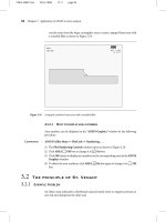
Figure 4.102 Window of Extrude Areas by XYZ Offset.
Ch04-H6875.tex 24/11/2006 17: 47 page 205
4.4 Mode analysis of a one-axis precision moving table using elastic hinges 205
Figure 4.103 ANSYS Graphics window.
Command
ANSYS Main Menu → Solution → Define Loads → Apply → Structural →
Displacement →On Areas
The window Apply U,ROT on Areas opens (Figure 4.104).
(1) Pick [A] the side wall for a piezoelectric actuator in Figure 4.105 and [B] the
bottom of the table. Then click [C] OK button and the window Apply U,ROT on
Areas opens (Figure 4.106).
(2) Select [D] All DOF in the box of Lab2 and, then, click [E] OK button. After these
steps ANSYS Graphics window is changed as shown in Figure 4.107.
4.4.3 Analysis
4.4.3.1 DEFINE THE TYPE OF ANALYSIS
The following steps are performed to define the type of analysis.
Command
ANSYS Main Menu →Solution →Analysis Type →New Analysis
The window New Analysis opens (Figure 4.108).
Ch04-H6875.tex 24/11/2006 17: 47 page 206
C
Figure 4.104 Window of Apply U,ROT on Areas.
B
A
Figure 4.105 ANSYS Graphics window.

Ch04-H6875.tex 24/11/2006 17: 47 page 207
4.4 Mode analysis of a one-axis precision moving table using elastic hinges 207
E
D
Figure 4.106 Window of Apply U,ROT on Areas.
Figure 4.107 ANSYS Graphics window.
Ch04-H6875.tex 24/11/2006 17: 47 page 208
208 Chapter 4 Mode analysis
B
A
Figure 4.108 Window of New Analysis.
(1) Check [A] Modal and, then, click [B] OK button.
In order to define the number of modes to extract, the following steps are
performed.
Command
ANSYS Main Menu →Solution →Analysis Type →Analysis Options
The window Modal Analysis opens (Figure 4.109).
(1) Check [A] Subspace of MODOPT and input [B] 3 in the box of No. of modes to
extract and click [C] OK button.
(2) Then, the window Subspace Modal Analysis as shown in Figure 4.110 opens.
Input [D] 5000 in the box of FREQE and click [E] OK button.
4.4.3.2 EXECUTE CALCULATION
Command
ANSYS Main Menu →Solution →Solve →Current LS
The window Solve Current Load Step opens.
(1) Click OK button and calculation starts. When the window Note appears, the
calculation is finished.
(2) Click Close button and the window is closed. The window /STATUS Command
is also open but this window can be closed by clicking the mark of X at the upper
right side of the window.

Ch04-H6875.tex 24/11/2006 17: 47 page 209
4.4 Mode analysis of a one-axis precision moving table using elastic hinges 209
C
B
A
Figure 4.109 Window of Modal Analysis.
4.4.4 Postprocessing
4.4.4.1 READ THE CALCULATED RESULTS OF THE FIRST MODE OF
VIBRATION
Command
ANSYS Main Menu →General Postproc →Read Results →First Set
4.4.4.2 PLOT THE CALCULATED RESULTS
Command
ANSYS Main Menu →General Postproc →Plot Results →Deformed Shape
Ch04-H6875.tex 24/11/2006 17: 47 page 210
210 Chapter 4 Mode analysis
E
D
Figure 4.110 Window of Subspace Modal Analysis.
The window Plot Deformed Shape opens (Figure 4.111).
(1) Select [A] Def+Undeformed and click [B] OK.
(2) The calculated result for the first mode of vibration appears on ANSYS Graphics
window as shown in Figure 4.112.
4.4.4.3 READ THE CALCULATED RESULTS OF THE SECOND AND
THIRD MODES OF VIBRATION
Command
ANSYS Main Menu →General Postproc →Read Results →Next Set
Perform the same steps described in Section 4.4.4.2 and the results calculated for the
higher modes of vibration are displayed as shown in Figures 4.113 and 4.114.
Ch04-H6875.tex 24/11/2006 17: 47 page 211

4.4 Mode analysis of a one-axis precision moving table using elastic hinges 211
B
A
Figure 4.111 Window of Plot Deformed Shape.
Figure 4.112 ANSYS Graphics window for the first mode.
4.4.4.4 ANIMATE THE VIBRATION MODE SHAPE
In order to easily observe the vibration mode shape, the animation of mode shape
can be used.
Command
Utility Menu →PlotCtrls →Animate →Mode Shape
Ch04-H6875.tex 24/11/2006 17: 47 page 212
212 Chapter 4 Mode analysis
Figure 4.113 ANSYS Graphics window for the second mode.
Figure 4.114 ANSYS Graphics window for the third mode.
Ch04-H6875.tex 24/11/2006 17: 47 page 213
4.4 Mode analysis of a one-axis precision moving table using elastic hinges 213
The window Animate Mode Shape opens (Figure 4.115).
A
B
Figure 4.115 Window of Animate Mode Shape.
(1) Input [A] 0.1 to Time delay box and click [B] OK button. Then the animation of
the mode shape is displayed in ANSYS Graphics window.
This page intentionally left blank
Ch05-H6875.tex 24/11/2006 17: 8 page 215
5
Chapter
Analysis for Fluid
Dynamics
Chapter outline
5.1 Introduction 215

5.2 Analysis of flow structure in a diffuser 216
5.3 Analysis of flow structure in a channel
with a butterfly valve 242
5.1
Introduction
V
arious fluids such as air and
liquid are used as an operating fluid
in a blower, a compressor, and a pump.
The shape of flow channel often deter-
mines the efficiency of these machines.
In this chapter, the flow structures in a
diffuser and the channel with a butterfly
valve are examined by using FLOTRAN
which is an assistant program of ANSYS.
A diffuser is usually used for increasing
the static pressure by reducing the fluid
velocity and the diffuser can be easily
found in a centrifugal pump as shown
in Figure 5.1.
Flow
Diffuser
Blades
Figure 5.1 Typical machines for fluid.
215
Ch05-H6875.tex 24/11/2006 17: 8 page 216
216 Chapter 5 Analysis for fluid dynamics
5.2
Analysis of flow structure in a diffuser
5.2.1 Problem description

Analyze the flow structure of an axisymmetric conical diffuser with diffuser angle
2θ =6
◦
and expansion ratio =4 as shown in Figure 5.2.
x
y
2θ = 6°
4.5D
E
Straight channel for entrance
9.55D
E
Diffuser region
50D
E
Straight channel for exit
Figure 5.2 Axisymmetrical conical diffuser.
Shape of the flow channel:
(1) Diffuser shape is axisymmetric and conical, diffuser angle 2θ =6
◦
, expansion
ratio =4.
(2) Diameter of entrance of the diffuser: D
E
=0.2 m.
(3) Length of straight channel for entrance: 4.5D
E
.
(4) Length of diffuser region: 9.55D
E

.
(5) Length of straight channel for exit: 50.0D
E
.
Operating fluid: Air (300 K)
Flow field: Turbulence
Velocity at the entrance: 20 m/s
Reynoldsnumber: 2.54 ×10
5
(assumed to setthediameter of the diffuser entrance
to a representative length)
Boundary conditions:
(1) Velocities in all directions are zero on all walls.
(2) Pressure is equal to zero at the exit.
(3) Velocity in the y direction is zero on the x-axis.
5.2.2 Create a model for analysis
5.2.2.1 SELECT KIND OF ANALYSIS
Command
ANSYS Main Menu →Preferences
Ch05-H6875.tex 24/11/2006 17: 8 page 217
5.2 Analysis of flow structure in a diffuser 217
The window Preferences for GUI Filtering opens (Figure 5.3).
(1) Check [A] FLOTRAN CFD and click [B] OK button.
A
B
Figure 5.3 Window of Preferences for GUI Filtering.
5.2.2.2 ELEMENT TYPE SELECTION
Command
ANSYS Main Menu →Preprocessor →Element Type →Add/Edit/Delete
Then the window Element Types as shown in Figure 5.4 opens.

(1) Click [A] add. Then the window Library of ElementTypes as shown in Figure 5.5
opens.
(2) Select [B] FLOTRAN CFD-2D FLOTRAN 141.
Ch05-H6875.tex 24/11/2006 17: 8 page 218
218 Chapter 5 Analysis for fluid dynamics
A
Figure 5.4 Window of Element Types.
C
B
Figure 5.5 Window of Library of Element Types.
(3) Click [C] OK button and click [D] Options button in the window of Figure 5.6.
(4) The window FLUID141 element type options opens as shown in Figure 5.7.
Select [E] Axisymm about X in the box of Element coordinate system and click
[F] OK button. Finally click [G] Close button in Figure 5.6.
Ch05-H6875.tex 24/11/2006 17: 8 page 219
5.2 Analysis of flow structure in a diffuser 219
D
G
Figure 5.6 Window of Element Types.
E
F
Figure 5.7 Window of FLUID141 element type options.
5.2.2.3 CREATE KEYPOINTS
To draw a diffuser for analysis, the method using keypoints on the window are
described in this section.
Ch05-H6875.tex 24/11/2006 17: 8 page 220
220 Chapter 5 Analysis for fluid dynamics
Command
ANSYS Main Menu →Preprocessor → Modeling →Create →Keypoints →In
Active CS

(1) The window Create Keypoints in Active Coordinate System opens (Figure 5.8).
A
B
Figure 5.8 Window of Create Keypoints in Active Coordinate System.
(2) Input [A] 0, 0 to X, Y, Z Location in active CS box, and then click [B] Apply
button. Do not click OK button at this stage. If OK button is clicked, the win-
dow will be closed. In this case, open the window Create Keypoints in Active
Coordinate System again and then perform step (2).
(3) In the same window, input the values of keypoints indicated in Table 5.1.
Table 5.1 Coordinates of keypoints
KP No. X Y
100
2 0.9 0
3 0.9 0.1
4 0 0.1
5 2.81 0
6 2.81 0.2
7 12.81 0
8 12.81 0.2
(4) After finishing step (3), eight keypoints appear on the window as shown in
Figure 5.9.
Ch05-H6875.tex 24/11/2006 17: 8 page 221
5.2 Analysis of flow structure in a diffuser 221
Figure 5.9 ANSYS Graphics window.
B
A
Figure 5.10 Window of Create Area
thru KPs.
5.2.2.4 CREATE
AREAS FOR DIFFUSER

Areas are created from the keypoints by
performing the following steps.
Command
ANSYS Main Menu →Preprocessor →
Modeling →Create →Areas →
Arbitrary →Through KPs
(1) The window Create Area thru KPs opens
(Figure 5.10).
(2) Pick keypoints 1, 2, 3, and 4 in Figure
5.9 in order and click [A] Apply button
in Figure 5.10. One area of the diffuser is
created on the window.
(3) Then another two areas are made on the
window by clicking keypoints listed in
Table 5.2.
(4) When three areas are made, click [B] OK
button in Figure 5.10.
Ch05-H6875.tex 24/11/2006 17: 8 page 222
222 Chapter 5 Analysis for fluid dynamics
Table 5.2 Keypoint numbers for making areas
Area No. KPs
1 1,2,3,4
2 2,5,6,3
3 5,7,8,6
A
Figure 5.11 Window of
Mesh Tool.
5.2.2.5 CREATE MESH IN LINES AND AREAS
Command
ANSYS Main Menu →Preprocessor →

Meshing →Mesh Tool
The window Mesh Tool opens (Figure 5.11).
(1) Click [A] Lines-Set box. Then the window Ele-
ment Size on Picked Lines opens (Figure 5.12).
(2) Pick Line 1 and Line 3 on ANSYS Graphics win-
dow (Line numbers and Keypoint numbers are
indicated in Figure 5.13) and click [B] OK button.
The window Element Sizes on Picked Lines
opens (Figure 5.14).
(3) Input [C] 15 to NDIV box and click [D] OK
button.
(4) Click [A] Lines-Set box in Figure 5.11 and pick
Line 2, Line 6, and Line 9 on ANSYS Graphics
window. Then click OK button.
(5) Input [E] 50 to NDIV box and [F] 0.2 to SPACE
in Figure 5.15. Then click [G] OK button. This
means that the last dividing space between grids
becomes one-fifth of the first dividing space on
Line 2. When Line 2 was made according to
Table 5.2, KP 2 was first picked and then KP 3.
So the dividing space of grids becomes smaller
towardKP3.
(6) In order to mesh all lines, input the values listed in
Table 5.3.
Command
ANSYS Main Menu →Preprocessor →
Meshing →Mesh Tool
The window Mesh Tool opens (Figure 5.16).
(1) Click Mesh on the window Mesh Tool in Figure
5.11 and the window Mesh Areas opens (Figure

5.16). Click [A] Pick All button when all areas are
divided into elements as seen in Figure 5.17.
Ch05-H6875.tex 24/11/2006 17: 8 page 223
5.2 Analysis of flow structure in a diffuser 223
B
Figure 5.12 Window of Element Size on Picked Lines.
KP1 KP2
KP3KP4
KP6
KP7
KP8
KP5
L1
L2
L3
L4
L5
L6
L7
L8
L9
L10
Figure 5.13 Keypoint and Line numbers for a diffuser.
Command
Utility Menu →PlotCtrls →Pan-Zoom-Rotate
The window Pan-Zoom-Rotate opens (Figure 5.18).
(1) Click [A] Box Zoom and [B] make a box on ANSYS Graphics window to zoom
up the area as shown in Figure 5.17. Then the enlarged drawing surrounded by
the box appears on the window as shown in Figure 5.19.