Engineering Analysis with Ansys Software Episode 2 Part 7 docx

Ch06-H6875.tex 24/11/2006 17: 48 page 304
304 Chapter 6 Application of ANSYS to thermo mechanics
Figure 6.70, click [A] Pick All in order to bring the frame shown in Figure 6.71. As
before, activate both [A] All DOF and TEMP and input [B] TEMP value =232
◦
C.
Clicking [C] OK applies temperature constraints on nodes at the bottom of the tank.
Now, it is necessary to rotate the WP to the pipe axis. From Utility Menu select
WorkPlane →Offset WP by Increments. Figure 6.73 shows the resulting frame.
A
Figure 6.73 Offset WP by Increments.
Ch06-H6875.tex 24/11/2006 17: 48 page 305
6.3 Steady-state thermal analysis of a pipe intersection 305
In degrees box input [A] XY =0 and YZ =−90 as shown. Having WP rotated
to the pipe axis, a local cylindrical coordinate system has to be defined at the origin
of the WP. From Utility Menu select WorkPlane → Local Coordinate Systems →
Create local CS →At WP Origin. The resulting frame is shown in Figure 6.74.
A
B
Figure 6.74 Create Local CS.
A
B
C
D
Figure 6.75 Select Entities.
From the pull down menu select [A] Cylin-
drical 1 and click [B] OK button to imple-
ment the selection. The analysis involves nodes
located on inner surface of the pipe. In order to
include this subset of nodes, from Utility Menu
select Select → Entities. Figure 6.75 shows the

resulting frame.
From the first pull down menu select [A]
Nodes, from the second pull down menu select
[B] By Location. Also, activate [C] Xcoor-
dinates button and [D] enter Min,Max =0.4
(inside radius of the pipe). All the four required
steps are shown in Figure 6.75. From ANSYS
Main Menu select Solution → Define Load →
Apply →Thermal →Convection →On nodes.
In the resulting frame (shown in Figure 6.67),
press [A] Pick All and the next frame, shown in
Figure 6.76, appears.
Input [A] Film coefficient =−2 and [B]
Bulk temperature =38 as shown in Figure 6.76.
Pressing [C] OK button implements the selec-
tions. The values inputted are taken from
Table 6.1. The final action is to select all enti-
ties involved with a single command. Therefore,
from Utility Menu select Select → Everything.
For the loads to be applied to tank and pipe
surfaces in the form of arrows from Utility Menu
Ch06-H6875.tex 24/11/2006 17: 48 page 306
306 Chapter 6 Application of ANSYS to thermo mechanics
A
B
C
Figure 6.76 Apply CONV on Nodes.
select PlotCtrls →Symbols. The frame in Figure 6.77 shows the required selection:
[A] Arrows.
From Utility Menu selecting Plot →Nodes results in Figure 6.78 where surface

loads at nodes as shown as arrows.
From Utility Menu select WorkPlane → Change Active CS to → Specified
Coord Sys in order to activate previously defined coordinate system. The frame
shown in Figure 6.79 appears.
Input [A] KCN (coordinate system number) =0 to return to Cartesian system.
Additionally from ANSYS Main Menu select Solution → Analysis Type → Sol’n
Controls. As a result, the frame shown in Figure 6.80 appears.
Input the following [A] Automation time stepping =On and [B] Number of
substeps =50 as shown in Figure 6.80. Finally, from ANSYS Main Menu select
Solve → Current LS and in the appearing dialog box click OK button to start the
solution process.
6.3.5 Postprocessing stage
When the solution is done, the next stage is to display results in a form required to
answer questions posed by the formulation of the problem.
Ch06-H6875.tex 24/11/2006 17: 48 page 307
6.3 Steady-state thermal analysis of a pipe intersection 307
A
Figure 6.77 Symbols.
Ch06-H6875.tex 24/11/2006 17: 48 page 308
308 Chapter 6 Application of ANSYS to thermo mechanics
Figure 6.78 Convection surface loads displayed as arrows.
A
Figure 6.79 Change Active CS to Specified CS.
From Utility Menu select PlotCtrls →Style →Edge Options. Figure 6.81 shows
the resulting frame.
Select [A] All/Edge only and [B] press OK button to implement the selection
which will result in the display of the “edge” of the object only. Next, graphic controls
ought to be returned to default setting. This is done by selecting from Utility Menu
PlotCtrls → Symbols. The resulting frame, as shown in Figure 6.82, contains all
default settings.

Ch06-H6875.tex 24/11/2006 17: 48 page 309
6.3 Steady-state thermal analysis of a pipe intersection 309
A
B
Figure 6.80 Solution Controls.
A
B
Figure 6.81 Edge Options.
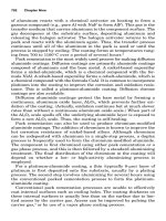
The first plot is to show temperature distribution as continuous contours. From
ANSYS Main Menu select General Postproc → Plot Results → Contour Plot →
Nodal Solu. The resulting frame is shown in Figure 6.83.
Select [A] Temperature and press [B] OK button as shown in Figure 6.83. The
resulting temperature map is shown in Figure 6.84.
Ch06-H6875.tex 24/11/2006 17: 48 page 310
310 Chapter 6 Application of ANSYS to thermo mechanics
Figure 6.82 Symbols.
Ch06-H6875.tex 24/11/2006 17: 48 page 311
6.3 Steady-state thermal analysis of a pipe intersection 311
A
B
Figure 6.83 Contour Nodal Solution Data.
Figure 6.84 Temperature map on inner surfaces of the tank and the pipe.
Ch06-H6875.tex 24/11/2006 17: 48 page 312
312 Chapter 6 Application of ANSYS to thermo mechanics
The next display of results concerns thermal flux at the intersection between
the tank and the pipe. From ANSYS Main Menu select General Postproc → Plot
Results →Vector Plot →Predefined. The resulting frame is shown in Figure 6.85.
A
B
C

Figure 6.85 Vector Plot Selection.
In Figure 6.85, select [A] Thermal flux TF and [B] Raster Mode. Pressing [C] OK
button implements selections and produces thermal flux as vectors. This is shown in
Figure 6.86.
6.4
Heat dissipation through ribbed surface
6.4.1
Problem description
Ribbed or developed surfaces, also called fins, are frequently used to dissipate heat.
There are many examples of their use in practical engineering applications such as
computers, electronic systems, radiators, just to mention a few of them.
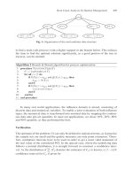
Figure 6.87shows a typical configuration and geometry of a fin made of aluminum
with thermal conductivity coefficient k =170 W/m K.
Ch06-H6875.tex 24/11/2006 17: 48 page 313
6.4 Heat dissipation through ribbed surface 313
Figure 6.86 Distribution of thermal flux vectors at the intersection between the tank and the pipe.
330
20 20 20
10
100
85
85
40
25
50
Figure 6.87 Cross-section of the fin.
The bottom surface of the fin is exposed to a constant heat flux of q =1000W/m.
Air flows over the developed surface keeping the surrounding temperature at
293 K. Heat transfer coefficient between the fin and the surrounding atmosphere
is h =40W/m

2
K.
Determine the temperature distribution within the developed surface.
6.4.2 Construction of the model
From ANSYS Main Menu select Preferences to call up a frame shown in Figure 6.88.
Ch06-H6875.tex 24/11/2006 17: 48 page 314
314 Chapter 6 Application of ANSYS to thermo mechanics
A
Figure 6.88 Preferences: Thermal.
Because the problem to be solved is asking for temperature distribution, there-
fore [A] Thermal is selected as indicated in the figure. Next, from ANSYS Main
Menu select Preprocessor → Element Type →Add/Edit/Delete. The frame shown
in Figure 6.89 appears.
A
Figure 6.89 Define element type.
Ch06-H6875.tex 24/11/2006 17: 48 page 315
6.4 Heat dissipation through ribbed surface 315
Click [A] Add button to call up another frame shown in Figure 6.90.
A
B
Figure 6.90 Library of Element Types.
In Figure 6.90, the following selections are made: [A] Thermal Mass → Solid
and [B] Tet 10node 87.FromANSYS Main Menu select Preprocessor → Material
Props →Material Models. Figure 6.91 shows the resulting frame.
A
Figure 6.91 Define Material Model Behavior.
From the right-hand column select [A] Thermal →Conductivity → Isotropic.
In response to this selection another frame, shown in Figure 6.92, appears.
Thermal conductivity [A] KXX =170 W/m K is entered and [B] OK button
clicked to implement the entry as shown in the figure.

The model of the developed area will be constructed using primitives and it is
useful to have them numbered. Thus, from ANSYS Utility Menu select PlotCtrls →
Numbering and check [A] the box area numbers on as shown in Figure 6.93.
Ch06-H6875.tex 24/11/2006 17: 48 page 316
316 Chapter 6 Application of ANSYS to thermo mechanics
A
B
Figure 6.92 Conductivity coefficient.
A
Figure 6.93 Numbering Controls.
From ANSYS Main Menu select Preprocessor →Modelling →Create →Areas
→Rectangle →By Dimensions. Figure 6.94 shows the resulting frame.
Input [A] X1 =−165; [B] X2 =165; [C] Y1 =0; [D] Y2 =100 to create rectan-
gular area (A1) within which the fin will be comprised. Next create two rectangles
Ch06-H6875.tex 24/11/2006 17: 48 page 317
6.4 Heat dissipation through ribbed surface 317
A
C
B
D
Figure 6.94 Create Rectangle by Dimensions.
at left and right upper corner to be cut off from the main rectangle. From ANSYS
Main Menu select Preprocessor →Modelling →Create →Areas →Rectangle →
By Dimensions. Figure 6.95 shows the resulting frame.
A
C
B
D
Figure 6.95 Rectangle with specified dimensions.
Figure 6.95 shows inputs to create rectangle (A2) at the left-hand upper corner

of the main rectangle (A1). They are: [A] X1 =−165; [B] X2 =−105; [C] Y1 =85;
[D] Y2 =100. In order to create right-hand upper corner rectangles (A3) repeat the
above procedure and input: [A] X1 =105; [B] X2 =165; [C] Y1 =85; [D] Y2 =100.
Now, areas A2 and A3 have to be subtracted from area A1. From ANSYS Main Menu
select Preprocessor → Modelling → Operate → Booleans → Subtract → Areas.
Figure 6.96 shows the resulting frame.
First, select area A1 (large rectangle) to be subtracted from and [A] click OK
button. Next, select two smaller rectangles A2 and A3 and click [A] OK button. A
new area A4 is created with two upper corners cut off. Proceeding in the same way,
areas should be cut off from the main rectangle in order to create the fin shown in
Figure 6.87.
Ch06-H6875.tex 24/11/2006 17: 48 page 318
318 Chapter 6 Application of ANSYS to thermo mechanics
A
Figure 6.96 Subtract Areas.
From ANSYS Main Menu select Prepro-
cessor → Modelling → Create → Areas →
Rectangle → By Dimensions. Figure 6.97
shows the frame in which appropriate input
should be made.
In order to create area A1 input: [A]
X1 =−145; [B] X2 =−125; [C] Y1 =40; [D]
Y2 =85. In order to create area A2 input:
[A] X1 =125; [B] X2 =145; [C] Y1 =40; [D]
Y2 =85. In order to create area A3 input: [A]
X1 =−105; [B] X2 =−95; [C] Y1 =25; [D]
Y2 =100. In order to create area A5 input:
[A] X1 =95; [B] X2 =105; [C] Y1 =25; [D]
Y2 =100.
From ANSYS Main Menu select Prepro-

cessor →Modelling → Operate → Booleans
→ Subtract → Areas. The frame shown in
Figure 6.96 appears. Select first area A4 (large
rectangle) and click [A] OK button. Next,select
areas A1, A2, A3, and A5 and click [A] OK
button. Area A6 with appropriate cut-outs is
created. It is shown in Figure 6.98.
In order to finish construction of the fin’s
model use the frame shown in Figure 6.97 and
make the following inputs: [A] X1 =−85; [B]
X2 =−75; [C] Y1 =25; [D]
Y2 =100. Area
A1 is created. Next input: [A] X1 =−65; [B]
A
C
B
D
Figure 6.97 Create rectangle by four coordinates.
X2 =−55; [C] Y1 =25; [D] Y2 =100 to create area A2. Next input: [A] X1 =−45;
[B] X2 =−35; [C] Y1 =25; [D] Y2 =100 to create area A3. Appropriate inputs
should be made to create areas, to be cut out later, on the right-hand side of the fin.
Thus inputs: [A] X1 =85; [B] X2 =75; [C] Y1 =25; [D] Y2 =100 create area A4.
Inputs: [A] X1 =65; [B] X2 =55; [C] Y1 =25; [D] Y2 =100 create area A5. Inputs
Ch06-H6875.tex 24/11/2006 17: 48 page 319
6.4 Heat dissipation through ribbed surface 319
Figure 6.98 Image of the fin after some areas were subtracted.
[A] X1 =45; [B] X2 =35; [C] Y1 =25; [D] Y2 =100 create area A7. Next, from
ANSYS Main Menu select Preprocessor → Modelling → Operate →Booleans →
Subtract →Areas. The frame shown in Figure 6.96 appears. Select first area A6 and
click [A] OK button. Then, select areas A1, A2, A3, A4, A5, and A7. Clicking [A]

OK button implements the command and a new area A8 with appropriate cut-outs is
created. In order to finalize the construction of the model make the following inputs
to the frame shown in Figure 6.97 to create area A1: [A] X1 =−25; [B] X2 =−15; [C]
Y1 =50; [D] Y2 =100. Inputs: [A] X1 =−5; [B] X2 =5; [C] Y1 =50; [D] Y2 =100
create area A2. Finally input [A] X1 =15; [B] X2 =25; [C] Y1 =50; [D] Y2 =100
to create area A3. Again from ANSYS Main Menu select Preprocessor →Modelling
→ Operate → Booleans → Subtract → Areas. The frame shown in Figure 6.96
appears. Select first area A8 and click [A] OK button. Next, select areas A1, A2, and
A3. Clicking [A] OK button produces area A4 shown in Figure 6.99. Figure 6.99
shows the final shape of the fin with dimensions as specified in Figure 6.87. It is,
however, a 2D model. The width of the fin is 100 mm and this dimension can be used
to create 3D model.
Figure 6.99 Two-dimensional image of the fin.
From ANSYS Main Menu select Preprocessor → Modelling → Operate →
Extrude → Areas → Along Normal. Select Area 4 (to be extruded in the direction
normal to the screen, i.e., z-axis) and click OK button. In response, the frame shown
in Figure 6.100 appears.
Ch06-H6875.tex 24/11/2006 17: 48 page 320
320 Chapter 6 Application of ANSYS to thermo mechanics
A
B
Figure 6.100 Extrude area.
Input [A] Length of extrusion =100 mm and [B] click OK button. The3D model
of the fin is created as shown in Figure 6.101.
Figure 6.101 Three-dimensional (isometric) view of the fin.
The fin is shown in isometric view without area numbers. In order to deselect
numbering of areas refer to Figure 6.93 in which box Area numbers should be
checked off.
From ANSYS Main Menu select Preprocessor → Meshing → Mesh
Attributes →Picked Volumes. The frame shown in Figure 6.102 is created.

Ch06-H6875.tex 24/11/2006 17: 48 page 321
6.4 Heat dissipation through ribbed surface 321
A
Figure 6.102 Volume Attributes.
Select [A] Pick All and the next frame, shown in Figure 6.103, appears.
Material Number 1 and element type SOLID87 are as specified at the beginning
of the analysis and in order to accept that click [A] OK button.
Now meshing of the fin can be carried out. From ANSYS Main Menu select
Preprocessor → Meshing → Mesh → Volumes → Free. The frame shown in
Figure 6.104 appears.
Select [A] Pick All option, as shown in Figure 6.104, to mesh the fin. Figure 6.105
shows the meshed fin.
6.4.3 Solution
Prior to running solution stage boundary conditions have to be properly applied. In
the case considered here the boundary conditions are expressed by the heat transfer
coefficient which is a quantitative measure of how efficiently heat is transferred from
fin surface to the surrounding air.
From ANSYS Main Menu select Solution → Define Loads → Apply →
Thermal →Convection →On Areas. Figure 6.106 shows the resulting frame.
Ch06-H6875.tex 24/11/2006 17: 48 page 322
322 Chapter 6 Application of ANSYS to thermo mechanics
A
Figure 6.103 Volume attributes with specified material and element type.
A
Figure 6.104 Mesh Volumes.
Ch06-H6875.tex 24/11/2006 17: 48 page 323
6.4 Heat dissipation through ribbed surface 323
Figure 6.105 View of the fin with mesh network.
A
Figure 6.106 Apply boundary conditions to

the fin areas.
Select all areas of the fin except the bot-
tom area and click [A] OK button. The frame
created as a result of that action is shown in
Figure 6.107.
Input [A] Film coefficient =40 W/m
2
K;
[B] Bulk temperature =293 K and click [C]
OK button. Next a heat flux of intensity
1000 W/m has to be applied to the base of the
fin. Therefore, from ANSYS Main Menu select
Solution → Define Loads →Apply →Ther-
mal → Heat Flux → On Areas. The resulting
frame is shown in Figure 6.108.
Select the bottom surface (base) of the fin
and click [A] OK button. A new frame appears
(see Figure 6.109) and the input made is as
follows: [A] Load HFLUX value =1000W/m.
Clicking [B] OK button implements the input.
All required preparations have been made
and the model is ready for solution. From
ANSYS Main Menu select Solution → Solve
→ Current LS. Two frames appear. One gives
a summary of solution options. After checking
correctness of the options, it should be closed
using the menu at the top of the frame. The
other frame is shown in Figure 6.110.
Clicking [A] OK button starts the solution
process.